Constructing IGA-suitable planar parameterization from complex CAD boundary by domain partition and global/local optimization
Abstract
In this paper, we propose a general framework for constructing IGA-suitable planar B-spline parameterizations from given complex CAD boundaries consisting of a set of B-spline curves. Instead of forming the computational domain by a simple boundary, planar domains with high genus and more complex boundary curves are considered. Firstly, some pre-processing operations including Bézier extraction and subdivision are performed on each boundary curve in order to generate a high-quality planar parameterization; then a robust planar domain partition framework is proposed to construct high-quality patch-meshing results with few singularities from the discrete boundary formed by connecting the end points of the resulting boundary segments. After the topology information generation of quadrilateral decomposition, the optimal placement of interior Bézier curves corresponding to the interior edges of the quadrangulation is constructed by a global optimization method to achieve a patch-partition with high quality. Finally, after the imposition of -continuity constraints on the interface of neighboring Bézier patches with respect to each quad in the quadrangulation, the high-quality Bézier patch parameterization is obtained by a -constrained local optimization method to achieve uniform and orthogonal iso-parametric structures while keeping the continuity conditions between patches. The efficiency and robustness of the proposed method are demonstrated by several examples which are compared to results obtained by the skeleton-based parameterization approach.
Keywords:
isogeometric analysis , analysis-suitable planar parameterization; complex CAD boundary , domain partition , global/local optimization1 Introduction
In isogeometric analysis (IGA) [16], the parameterization of the computational domain corresponds to the mesh generation in finite element analysis. Consequently, it has a great effect on the subsequent analysis accuracy and efficiency [7, 47, 35]. As proposed in [48], an analysis-suitable parameterization of the computational domain should satisfy three requirements: 1) it has no self-intersections, i.e, the mapping from the parametric domain to the physical domain should be injective; 2) the iso-parametric elements should be as uniform as possible; 3) the iso-parametric structure should be as orthogonal as possible. From the given boundary information with spline representations, several approaches such as constrained optimization methods [49], variational harmonic methods [50], divide-and-conquer techniques [45], the Teichmüller mapping method [29], skeleton-based decomposition method [52], multi-patch parameterization method [4] , and parameterization with non-standard B-splines (i.e, T-splines [54], THB-splines [11], PHT/RHT-splines [31, 32, 33, 34], Powell-Sabin splines [40] and subdivision surfaces [36, 37]), have been proposed to address the parameterization problem of the computational domain. However, most of the above methods only focus on the computational domain with simple boundaries. The construction of analysis-suitable parameterizations of complex computational domains with standard B-spline boundaries remains one of the most significant challenges in IGA.
In this paper, a general framework for constructing IGA-suitable planar parameterization from complex CAD boundaries consisting of standard B-spline curves is proposed. Instead of the computational domain formed by four boundary curves, the planar domains with high genus and more complex boundary curves are considered. Our main contributions can be summarized as follows:
- 1.
We propose a general framework for IGA-suitable planar parameterizations from complex CAD boundaries by domain partition and global/local optimization.
- 2.
Given a complex planar domain bounded by B-spline curves, a novel method is proposed to construct four-sided patch partitions with high quality by global optimization and quad-meshing with few singularities.
- 3.
A -constrained local optimization approach is proposed to construct the Bézier patch with respect to each quad in the quadrangulation achieving high-quality iso-parametric structures while keeping the continuity constraints between patches.
The rest of the paper is structured as follows. Some related work on parameterization of the computational domain are reviewed in Section 2. Preliminary properties of Bernstein polynomials and an overview of the proposed framework is given in Section 3. Several pre-processing operations, including Bézier extraction and Bézier subdivision, are presented in Section 4. Section 5 describes the topology information generation and interior Bézier boundary construction for the quadrilateral high-quality patch partition by the global optimization approach. A local optimization method for high-quality Bézier patch parameterizations with continuity constraints is proposed in Section 6. Some parameterization examples are presented in Section 7. To demsonstrate the effectiveness of the proposed method, the results are compared to results obtained by the skeleton-based approach. Finally, we conclude this paper and outline future work in Section 8.
2 Related work
Currently, the related work on parameterization of the computational domain in IGA can be classified into four categories: (1) analysis-aware optimal parameterization; (2) volumetric spline parameterization from boundary triangulation; (3) analysis-suitable planar parameterization; (4) analysis-suitable volumetric parameterization from spline boundaries .
Analysis-aware optimal parameterization: E. Cohen et al. [7] proposed the concept of analysis-aware modeling, in which the parameters of CAD models are selected to facilitate isogeometric analysis. Xu et al. [47] showed that the quality of parameterization has a great impact on the analysis results and the efficiency. Pilgerstorfer and Jüttler [35] showed that the condition number of the stiffness matrix, which is a key factor for the stability of the linear system, depends strongly on the quality of the domain parameterization.
Volumetric spline parameterization from boundary triangulation: Using volumetric harmonic functions, Martin et al. [24] proposed a fitting method for triangular meshes by B-spline parametric volumes. In [10], a method is proposed to construct trivariate T-spline volumetric parameterizations for genus-zero solids based on an adaptive tetrahedral meshing and mesh untangling technique. Zhang et al. proposed a robust and efficient approach to construct injective solid T-splines for genus-zero geometries from a boundary triangulation [53]. Chan et al. proposed a volumetric parameterization method with PHT-splines from the level-set boundary representation [6]. For meshes with arbitrary topology, volumetric parameterization methods are proposed from the Morse theory [44] and Boolean operations [22].
Analysis-suitable planar parameterization: The boundary in CAD is usually provided in spline form. Xu et al. proposed a constrained optimization method to construct injective planar parameterizations [48]. Gravessen et al. [13] investigated the planar parameterization problem within a general non-linear optimization framework, in which several objective functions related to the parameterization quality are introduced. Xu et al. proposed a skeleton-guided domain decomposition method for planar parameterization with -continuity between patches [52]. Speleers and Manni proposed a parameterization method with Powell-Sabin splines defined on triangulation [40]; truncated hierarchical B-splines are used for the planar parameterization problems in [11]. Nian and Chen [29] proposed an approach for planar domain parameterization based on Teichmüller mapping, which can generate a bijective high-quality parameterization from four specified boundary curves. For the multi-patch parameterization problem, Buchegger and Jüttler [4] proposed a systematic method to explore the different possible parameterizations of a planar domain by collections of quadrilateral patches. For the geometrically continuous spline space over multi-patch domains, Kapl et al. proposed the construction of geometrically continuous isogeometric functions which are defined on two-patch domains [17]. Bases for bicubic and biquartic geometrically continuous isogeometric functions on bilinearly parameterized multi-patch domains are constructed in [18] ; Mourrain et al. analyzed the space of geometrically continuous piecewise polynomial splines for rectangular and triangular patches with arbitrary topology and general rational transition maps [25]; Buchegger et al. constructed the truncated hierarchical B-spline basis for the space of adaptively refined spline functions on multi-patch domains with enhanced smoothness across interfaces [3]. Overall, it is still an open problem how to construct analysis-suitable planar parameterization from complex CAD boundary.
Analysis-suitable volumetric parameterizations from spline boundary: A variational approach for constructing NURBS parameterizations of swept volumes is proposed by M. Aigner et al [1]. Xu et al. proposed a constrained optimization framework to construct analysis-suitable volume parameterizations [49]. Spline volume faring is proposed by Pettersen and Skytt to obtain high-quality volume parameterization [38]. The construction of conformal solid T-splines from boundary T-spline representations is studied by using octree structure and boundary offset [54]. In [50], a variational harmonic method is proposed to construct analysis-suitable parameterizations of computational domains from given CAD boundary information. Wang and Qian proposed an efficient method by combining divide-and-conquer, constraint aggregation and the hierarchical optimization technique to obtain valid trivariate B-spline solids from six boundary B-spline surfaces [45]. Analysis-suitable trivariate NURBS representations of composite panels is constructed with a new curve/surface offset algorithm [28]. Xu et al. proposed a two-stage scheme to construct the analysis-suitable NURBS volumetric parameterization by a uniformity-improved boundary reparameterization method [51]. Recently, given a template domain, B-spline based consistent volumetric parameterization is proposed for a set of models with similar semantic features [46].
3 Preliminary properties of Bernstein polynomials and framework overview
3.1 Preliminary properties of Bernstein polynomials
Since some properties of Bernstein polynomials [14] will be applied in our framework, they are reviewed subsequently.
Lemma 3.1.
Product of Bernstein polynomials
| (1) |
Lemma 3.2.
Integration of Bernstein polynomials
| (2) |
Lemma 3.3.
Degree elevation of Bernstein polynomials
| (3) |
Proposition 3.4.
Let and be a parametric function defined by
where and are scale values. Then the product of and can be defined as
| (4) |
where

(a) boundary Bézier curves

(b) discrete boundary

(c) quad meshing result

(d) segmentation curves

(e) parameterization result

(f) Jacobian colormap
3.2 Framework overview
The problem investigated in this paper can be stated as follows: Given a planar region bounded by a set of B-spline curves, construct an analysis-suitable planar B-spline parameterization. In other words: How can several B-spline patches be constructued to fill the computational domain bounded by B-spline curves? In order to address the above problem, a general framework is proposed which consists of the following four steps illustrated in Fig. 1:
- 1.
- 2.
Topology information generation of quadrilateral decomposition (Section 5.1): From the discrete boundary obtained by connecting the ending control points of each Bézier curve as shown in Fig. 1(b), approximate convex decomposition and pattern based quad mesh generation are employed to generate the topology information of the quadrilateral decomposition of the computational domain;
- 3.
Construction of the quadrilateral patch partition by global optimization (Section 5.2 and Section 5.3): After the topology partition is obtained, the Laplacian smoothing method is used to improve the quad mesh quality ( Fig. 1(c)); then the optimal geometry of the interior B-spline curves corresponding to the interior edges of the quadrangulation are obtained by a global optimization method to achieve a high-quality patch-partition ( Fig. 1(d)).
- 4.
High-quality patch parameterization by local optimization (Section 6): The Bézier patch with respect to each quad in the quadrangulation is obtained by local optimization to achieve uniform and orthogonal iso-parametric structures while keeping the continuity conditions between patches; an approach for detecting and recovering of invalid Bézier patches is also proposed to guarantee the injectivity of the resulting parameterization ( Fig. 1(e) and Fig. 1(f)).
4 Pre-processing of input boundary curves for high-quality parameterization
In order to achieve a high-quality parameterization of the computational domain, special treatment of input boundary curves are needed.
In IGA, the standard computational element is the sub-patch corresponding to the knot interval in the definition of the B-spline planar surface. In our parameterization framework, the input boundary B-spline curves will be segmented firstly with the Bézier extraction technique [2, 14], in which the piecewise B-spline representation is converted into Bézier form. The B-spline basis defined on a knot vector can be written as a linear combination of the Bernstein polynomials, that is,
| (5) |
where denotes the Bézier extraction operator and are the Bernstein polynomials which are defined on . The conversion matrix is sparse and its entries can be obtained by multiple knot insertion, which can be performed by Boehm’s algorithm. Details on the Bézier extraction can be found in [2, 14].
With the conversion matrix , the Bézier extraction of the B-spline curves can be represented by
| (6) |
denoting the control points of the B-spline curve, and are the control points of the extracted Bézier curve.
After Bézier extraction, most of the resulting Bézier curves have an ideal shape for the parameterization. However, in some cases, there might be some Bézier curves with complex shapes, which require further division. In order to obtain satisfactory curve segments, we will perform the Bézier subdivision process based on the distance estimation between Bézier curves and its control polygon [42, 26]. Let be the average length of the lines connecting the starting control points and ending control points of all the extracted Bézier curves from the input boundary. The corresponding termination criterion for this Bézier subdivision process can be described as follows:
Termination criterion. The maximal distance between the Bézier curve and the straight line connecting its starting control point and ending control point is smaller than .
It should be mentioned that is determined by the input boundary and is kept unchanged during the subdivision process. From the above termination criterion, the Bézier curve will be subdivided into two Bézier segments at if is larger than . If , and
then
| (7) |
where is the number of times the Bézier curve must be subdivided in order to satisfy the termination criterion [42, 26]. Fig. 2 shows an example of the Bézier subdivision, in which a Bézier curve with concave shape is subdivided into two Bézier segments for the subsequent high-quality parameterization process.

(a) original Bézier curve

(b) Bézier subdivision
5 Four-sided partition of the computational domain by global optimization
After the pre-processing operation for the given boundary curves, we will now propose a global optimization method to construct the four-sided curved partition of the computational domain. Three steps are required to address this problem: Firstly, we generate the topology information of the quadrilateral decompositions. Afterwards, the Laplacian mesh smoothing method is employed to improve the quad mesh quality. Finally, the optimal shape of the interior B-spline curves corresponding to the interior edges of the quadrangulation are obtained by a global optimization method.
5.1 Topology generation of quadrilateral decomposition

(a) input discrete boundary

(b) quasi-convex polygon decomposition

(c) quad-meshing result by our method with elements and irregular vertices

(d) meshing result by the method in [23] with elements and irregular vertices
In this subsection, we will describe how to generate the topology information of quadrilateral decompositions from the boundary curves of the computational domain. The main steps include:
- 1.
- 2.
Convert the multiply-connected regions into simply-connected regions as presented in Appendix I (see Fig. 4);
- 3.
- 4.
The proposed method in [41] can produce patterns with minimal number of irregular vertices, which are constructed by solving a set of small integer linear programs. As shown in Fig. 3, our framework can generate high-quality quad-meshing results with fewer irregular vertices compared to the method in [23]. Furthermore, the patterns proposed in [41] only introduce irregular vertices with valence or , which guarantees the solution existence for planar parameterization around the irregular vertex as shown in Section 6.1.3.

(a) multiply-connected domain

(b) simply-connected domain
5.2 Laplacian smoothing method
Since the quad-meshing quality significantly affects the final parameterization results, we adapt an iterative Laplacian smoothing method to improve the quality of the quad mesh. In every iteration, each internal mesh vertex is moved to the centroid of its neighbor vertices, i.e.
| (8) |
in which is the number of neighbor vertices of the internal mesh vertex with location , and the superscript is the iteration counter. This iteration is terminated according to the following termination rules:
| (9) |
where is the total number of mesh vertices, and is the specified tolerance value (0.001).
By the Laplacian smoothing method, we can improve the quad-mesh quality towards equilibrating the element size globally as shown in Fig. 3(c).
5.3 Construction of segmentation curves between patches
After constructing the quad mesh of the discrete computational domain, we construct the segmentation curves between patches corresponding to each quad. The segmentation curves interpolate two vertices on the quad mesh as shown in Fig. 5(a). Furthermore, for a planar computational domain, the shape of the segmentation curves has a great effect on the uniformity of the patch-size. Hence, we propose a global optimization method to construct the optimal shape of the segmentation curves.

(a) segmentation curves(red) w.r.t quad edges( black)

(b) segmentation curve at a singular vertex with
There are three objective functions: The first term is related to the uniformity of the patch-size; the second term is related to the shape quality of the segmentation curves; the third term is related to the tangent constraints of the segmentation curves at quad-mesh vertices.
For the uniformity of the patch-size, we propose a new metric related to the patch-area. It is obvious that the area of a planar region only depends on the shape of the boundary curves. In fact, for computing the area of the planar region bounded by Bézier curves, we have the following proposition.
Proposition 5.1.
For the planar region bounded by Bézier curves
in which is the control point, , , the area of the planar region is the sum of integrals as follows:
| (10) |
in which
| (11) |
| (12) |
Proposition 12 can be proved by Green’s formula [5] and the properties of Bernstein polynomials, which are described in subsection 3.1.
From Proposition 12, we define the uniformity metric for the Bézier patches constructed from the quad mesh . The uniform patch structure over the quad mesh means that each patch defined on each quad element in has the same area. In probability theory and statistics, the variance measures how far a set of numbers is spread out. A variance of zero indicates that all the values are identical. Hence, the uniformity of the patch structure requires the variance between each patch to be as small as possible. Suppose that is the area of the -th patch bounded by four Bézier curves, and is the average patch area in the patch structure over the quad mesh , i.e.
then the uniformity metric is defined as the variance of ,
| (13) |
in which is the number of Bézier patches in the patch structure , is the area of the patch structure bounded by the given set of B-spline curves. and can be computed according to the area formula presented in Proposition 12.
For the term related to the shape quality of the segmentation curves, the corresponding objective function is defined as a combination of the stretch energy and the strain energy,
| (14) |
in which and are positive weights. If , then the resulting segmentation curves have smaller stretch energy, which measures the length of a curve. If , we obtain segmentation curves with smaller strain energy, which is a measures of the curve’s bending.
For the term related to the tangent vector requirements of segmentation curves at the quad-mesh vertex with valence , we define the following objective function,
| (15) |
where is the tangent vector of the segmentation curve at the quad-mesh vertex , and as shown in Fig. 5(b). At regular vertices with valence , the minimization of will achieve quasi- and quasi-orthogonal segmentation curves, which is a basic requirement for analysis-suitable parameterization.
Combining the optimization terms defined in (13), (14) and (15), we construct an objective function as follows,
| (16) |
in which , and are positive weights for the balance between the shape quality metric, uniformity metric and the metric for tangent constraints. In order to achieve quasi- and quasi-orthogonal segmentation curves, is usually much larger than and .
The segmentation curves are obtained by solving the non-linear optimization problem
| (17) |
in which the design variables are the control points of the segmentation curves .
The scale of the optimization problem in (17) depends on the number and the degree of the Bézier segmentation curves. The L-BFGS method is adopted to obtain the optimal solution, which is a quasi-Newton method to solve unconstrained nonlinear minimization problems. In the L-BFGS method, we approximate the inverse Hessian matrix of the objective function in (17) by a sequence of gradient vectors from previous iterations. For more details, the reader can refer to [30].

Remark 5.1. The interior segmentation curves are called valid if there are no intersections between them except the connecting control points. That is, for each interior segmentation curve , , it has no intersections with its neighboring segmentation curves , , , and as shown in Fig. 6. In particular, we can derive the following sufficient conditions such that has no intersections with :
in which is the control point of segmentation curve . That is, if the triangles formed by the control points of do not intersect with the other triangles formed by the control points , then has no intersections with . These sufficient conditions can be integrated with the optimization problem (17) to generate valid interior segmentation curves.
6 High-quality patch parameterization by local constrained optimization
After the four-sided patch partition is generated, we next construct the inner control points for each Bézier patch. One basic requirement is that the resulting domain parameterization satisfies the continuity constraints. In this paper, we propose an efficient patch-wise local optimization method to construct high-quality patch parameterizations with continuity constraints. The main framework for each local patch construction is summarized as follows:
- 1.
Construct the boundary control points on the second layer of the control mesh for each patch by orthogonality optimization and impose continuity constraints to achieve a near-orthogonal iso-parametric structure at common segmentation curves as described in subsection 6.1;
- 2.
Construct interior control points for each patch by solving a linear system related to efficient energy-minimizing scheme as presented in subsection 6.2;
- 3.
Find the invalid patches on the parameterization and recover the patch validity by repositioning the control points by a local optimization method as described in subsection 6.3.
6.1 Construction of boundary second-layer control points with orthogonality optimization and continuity constraints
In this section, we will construct the boundary control points on the second layer of the control mesh, i.e , , , , and , to satisfy the orthogonality and continuity requirements. The construction procedures involves:
- 1.
Initial construction: Construct the initial control points on the second layer of the control mesh for each patch by orthogonality optimization as described in subsection 6.1.1;
- 2.
Imposition of -continuity: In the regular region, adjust the boundary control points on the second layer of the control mesh for each patch to achieve -continuity. Therefore, the Lagrange-multiplier method is employed as proposed in subsection 6.1.2 ;
- 3.
Imposition of -continuity: In the irregular region, adjust the 1-neighbor control points around the irregular vertex to satisfy the general -continuity constraints by solving linear system as described in subsection 6.1.3 .
In the following subsections, some details will be described for each step.
6.1.1 Initial construction by orthogonality optimization
Firstly, we will describe the initial construction by orthogonality optimization. Without loss of generality, we firstly construct the initial position of for the Bézier patch :
In order to achieve a near-orthogonal isoparametric structure on the boundary , the final position of is obtained by solving the following optimization problem
| (18) |
in which
| (19) |
| (20) |
Solving the similar optimization problems as (18) yields the position of , and for each patch, which requires adjustment to achieve continuity.
6.1.2 construction in the regular region
In order to ensure that the joint two Bézier patches and in the regular region satisfy continuity, the control mesh near the common segmentation curve with control points should satisfy the following conditions:
| (21) |
in which is the number of segmentation curves, and are the one-neighbor control points of the joint Bézier patches along the segmentation curve (see Fig. 7).
The problem to impose -continuity can be formulated as follows: Minimize the change of related control points along the segmentation curves (except the one-neighbor control points around the irregular vertex) such that they satisfy the -constraints. In the following, we will solve this constrained optimization problem using the Lagrange multiplier method.
In order to minimize the change of all the related control points along the segmentation curves, the optimization term is defined as
| (22) |
in which is the number of segmentation curves, and are the initial control points constructed by the approach in subsection 6.1.1.
The unknown variables in the constrained optimization problem (23) are the control points and . A necessary condition for , and to be a solution of (23) is that the corresponding partial derivatives vanish, that is,
| (24) |
Methods such as Gauss elimination can be employed to solve the linear system (24).
The proposed least-square scheme leads to the boundary control points on the second layer of control mesh for each Bézier patch, which satisfies the -continuity requirements.
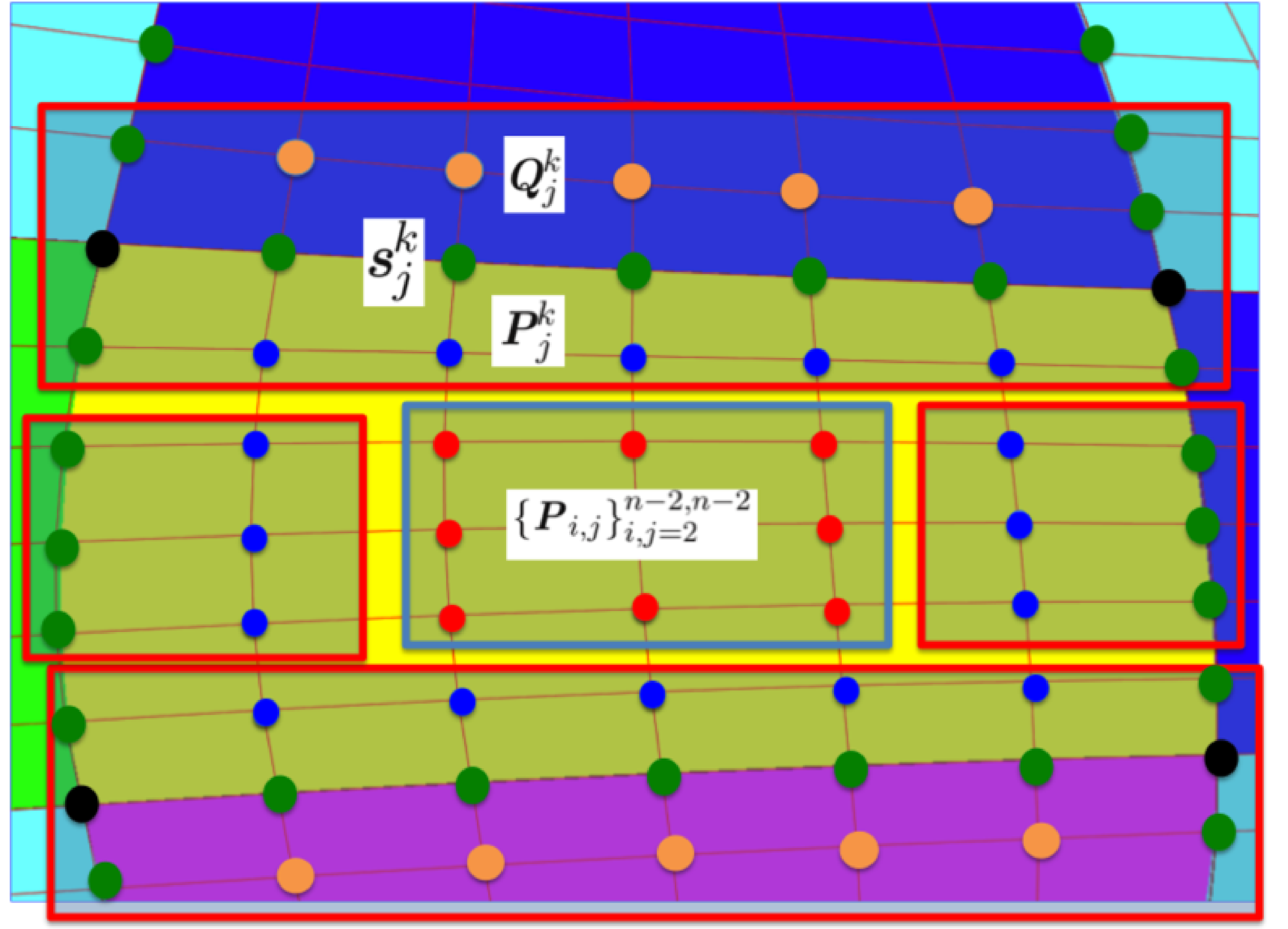

6.1.3 construction around irregular vertex
For the irregular vertices with non-four-valence on the quad mesh, some special treatments should be done in order to achieve continuity at ; continuity means -continuity of the parameterization maps through the composition with transition maps across the common edges of the patches. It differs from the continuity of the (planar) surfaces, which are the image of these parameterizations.
According to the pattern-based construction method of topology information described in Section 5.1 , there are only irregular vertices of valence or . Without loss of generality as shown in Fig. 8 , suppose that there are Bézier patches of degree meeting at the common control points , ( or ). With the Bézier segmentation curves constructed in Section 5.3, we construct the control points , which are nearest to the irregular vertex among the inner control points of , to satisfy the general continuity constraints. Specifying the transition map in the conditions proposed in [25], the continuity constraints around the irregular vertex can be obtained as follows,
| (25) | |||
| (26) |
Eq.(25) and Eq. (26) can be deduced from Eq. (13) and the system after Eq. (22) in [25], where the derivatives for the functions are expressed in terms of the control points of the Bézier patches. The similar -continuity constraints can be found in [19, 20].
The control points of the segmentation curves are fixed, , . In order to satisfy the first condition (25) of continuity, we firstly determine the values of and by solving a linear system (25) for a specified . Then, the unknown control points are determined according to the second condition (26), which can be rewritten as a linear system,
| (27) |
in which , .
Proposition 6.1.
6.2 Local linear-energy-minimizing method for constructing inner control points
In this section, we will propose a local linear-energy-minimizing method for constructing interior control points of each patch with prescribed boundary two-layer control points as shown in Fig.7. This problem can be stated as follows: Given the boundary control points on the first two layers of the control mesh, i.e. ,, , , , and of a tensor Bézier patch , find the remaining interior control points , such that the following energy function is minimal,
| (29) |
The energy function is related to the orthogonality and uniformity of the iso-parametric structure on the Bézier surface [50]. and are positive weights to control the parameterization results: if is big, then the resulting iso-parametric structure has better orthogonality; if has a small value, then we can obtain an iso-parametric grid with better uniformity.
Different from the non-linear optimization method [50], with prescribed boundary two-layer control points, we will give the sufficient and necessary condition for the interior control points of the Bézier patch with minimal energy in the following proposition.
Proposition 6.2.
Given the boundary control points ,, , , , and of a tensor product Bézier surface , then has minimal energy if and only if the remaining inner control points satisfy
| 0 | (30) | ||||
where
A proof of Proposition 6.2 is given in Appendix II.
Since the energy functional has a lower bound, the corresponding energy-minimizing Bézier surface always exists. From Proposition 6.2, for each unknown interior control point, an equation is obtained. Hence, we can get a linear system with equations and variables as follows,
in which M is the coefficient matrix determined by Eq.(30), is the set of unknown interior control points, B is the right-hand side related to the specified control points on the first two layers of control mesh.
Solving this linear system, the unknown interior control points can be represented as a linear combination of the specified control points on the first two layers of the control mesh. Furthermore, as each Bézier patch in the computational domain has the same coefficient matrix M, we only compute the inverse of M once and reuse it for the remaining Bézier patches in the computational domain.
6.3 Local optimization approach for injective parameterization
A parameterization is valid if it has no self-intersections, meaning the mapping from the parametric domain to the computational domain is injective. After the local energy-minimizing patch construction described in Section 6.2 , usually most of the Bézier patches are valid. However, for a few patches the resulting parameterization may still have self-intersections. In this section, we will firstly identify these invalid patches and subsequently reposition their control points to recover validity.
A parameterization is injective if its Jacobian is positive everywhere [13, 48]. For a planar Bézier surface , its Jacobian can be represented as a high-order Bernstein polynomial [13, 48],
| (31) |
Hence, the Jacobian is bounded by
| (32) |
Our invalid-patch-finding method can be described as follows: For each Bézier patch on the computational domain , we compute its Jacobian coefficients according to Eq. (31); if , then is called valid patch; otherwise, is called invalid patch.
After finding all the invalid patches on the planar parameterization, we will repair the invalid patch locally by repositioning its internal control points such that all the Jacobian coefficients are positive. Gravessen et al. [13] and Xu et al. [48] investigated this problem with a general non-linear constrained optimization framework,
| (33) |
in which is defined as (29).
In contrast to the proposed optimization method in [13, 48], we solve this constrained optimization problem using the classical logarithmic-barrier method [9, 12, 39]:
| (34) |
where is a positive penalty parameter.
The results from our experiments indicate that the injective parameterization can be achieved by the log-barrier method, although without theoretical guarantee of injectivity. Since the corresponding non-linear optimization (34) is only performed on very few local invalid Bézier patches with limited number of design variables, we can obtain the final optimized parameterization efficiently.
Remark 6.1. For a general framework to obtain an injective parameterization, the optimization problem (33) can be generalized as follows :
in which is defined in (31).
Remark 6.2. Teichmüller mapping method proposed in [29], which has theoretical guarantees of injectivity, can be used to improve the proposed local optimization scheme .
Remark 6.3. Due to the -constraints and the local optimization method in our framework, the minimum degree of the Bézier patches to guarantee a solution is 4. If the degree of the input boundary is smaller than 4, degree-elevation operation should be performed.
7 Examples and comparison
Starting from a set of B-spline curves as input, the proposed framework for analysis-suitable planar parameterization has been implemented as a plugin in the AXEL 11 1 http://axel.inria.fr/ platform. In this section, five parameterization examples are presented to show the effectiveness of the proposed method. The comparison with the skeleton-based parameterization method [52] is also performed for three parameterization examples.
7.1 Metrics for quality evaluation
In order to evaluate the quality of the planar parameterization results, we use the scaled Jacobians and the condition number of the Jacobian matrices as two important criteria. The scaled Jacobian at can be computed as follows,
| (35) |
A parameterization is said to be inverted if its Jacobians at some place is less or equal to zero. The minimal requirement for a planar parameterization to be suitable for isogeometric analysis is that all scaled Jacobians are as close as possible to 1.0.
The condition number of a Jacobian matrix is another important evaluation criteria, given by
| (36) |
in which
| (37) |
The Frobenius norm of is defined as . It can be easily proven that the minimum of is 2.0. For the quality evaluation of planar parameterization, the condition number is smaller, the optimization is better.
7.2 Effect of quad meshing
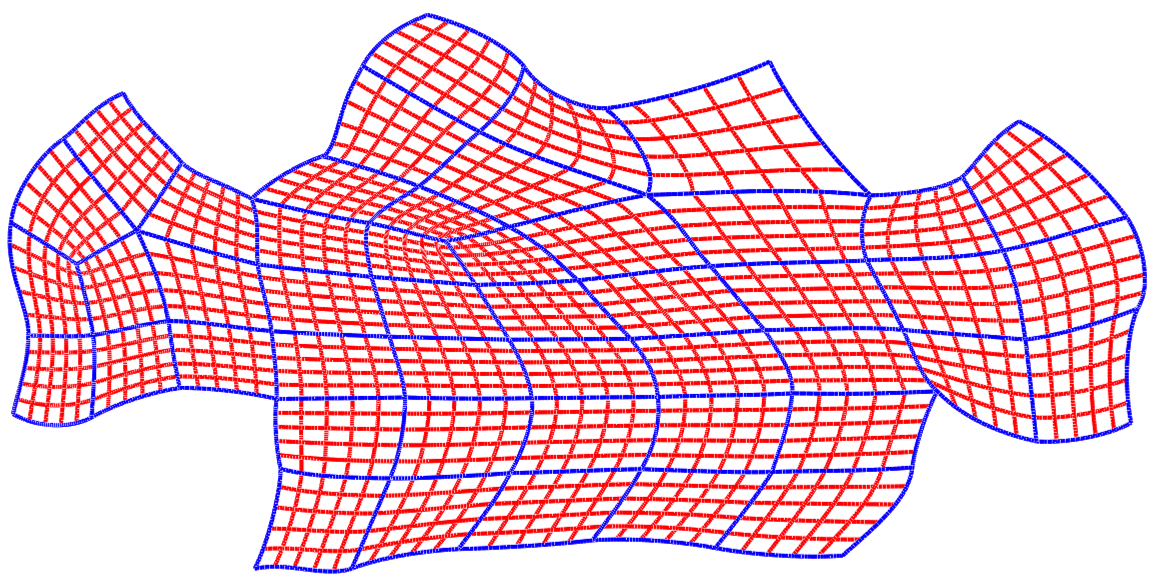
In the proposed framework, the quad-meshing step has a great effect on the final parameterization results. Furthermore, the quad-meshing results depend on the approximate convex decomposition of the input computational domain. For the approximate convex decomposition method in [21], if different non-concavity tolerances are specified, different number of approximate convex sub-domain can be obtained. Hence, from the same input boundary Fig. 9 (a), different quad-meshing results can be generated from different selection of non-concavity tolerance as shown in Fig. 9(b) with and Fig. 9(e) with . For a smaller non-concavity tolerances , we can obtain a quad-meshing result with more quad elements and more irregular vertices. Moreover, the corresponding scaled Jacobian colormap of the parameterization in Fig. 9 (c) and Fig. 9 (g) are depicted in Fig. 9 (d) and Fig. 9 (h).

(a) boundary Bézier curves

(b) quad meshing result I with
(c) parameterization result I

(d) Jacobian colormap I

(e) quad meshing result II with

(f) segmentation curves II

(g) parameterization result II

(h) Jacobian colormap

(i) boundary with more Bézier curves

(j) quad meshing result III

(k) parameterization result III

(l) Jacobian colormap III
The number of Bézier segments for the same input boundary also influences the final parameterization results. For the same input boundary with different number of Bézier segments, different quad-meshing result will be obtained leading to different parameterizations. For instance, the same boundary with different number of Bézier segments is shown in Fig. 9 (i). The corresponding quad-meshing result is presented in Fig. 9 (j), and the final parameterization and the corresponding scaled Jacobian colormap are illustrated in Fig. 9 (k) and Fig. 9 (l) respectively. Quantitative data of three parameterization results presented in Fig. 9 (c), Fig. 9 (g) and Fig. 9 (k) are listed in Table 1.
| Example | # Con. | #Patch | Scaled Jacobian | Condition number | ||||||
|---|---|---|---|---|---|---|---|---|---|---|
| Max | Average | Min | Max | Average | Min | |||||
| Fig. 9 (c) | 817 | 47 | 1.000 | 0.9054 | 0.431 | 4.72 | 2.41 | 2.00 | ||
| Fig. 9 (g) | 841 | 49 | 1.000 | 0.9024 | 0.263 | 7.62 | 2.53 | 2.00 | ||
| Fig. 9 (k) | 923 | 57 | 1.000 | 0.9279 | 0.582 | 3.86 | 2.36 | 2.00 | ||

(a) boundary Bézier curves

(b) discrete boundary

(c) quad meshing result

(d) segmentation curves

(e) parameterization result

(f) Jacobian colormap

(g) extracted skeleton [52]

(h) skeleton-based parameterization [52]

(i) Jacobian colormap of (h)

(a) boundary Bézier curves

(b) discrete boundary

(c) quad meshing result

(d) segmentation curves

(e) parameterization result

(f) Jacobian colormap

(g) extracted skeleton [52]

(h) skeleton-based parameterization [52]

(i) Jacobian colormap of (h)

(a) boundary Bézier curves

(b) discrete boundary

(c) quad meshing result

(d) segmentation curves
(e) parameterization result

(f) Jacobian colormap

(g) extracted skeleton [52]

(h) skeleton-based domain partition[52]

(i) skeleton-based parameterization [52]

(j) Jacobian colormap of (i)
7.3 Comparison with skeleton-based parameterization method
In order to show the effectiveness of the proposed approach, three examples are presented to compare the proposed method with the skeleton-based domain decomposition method [52].
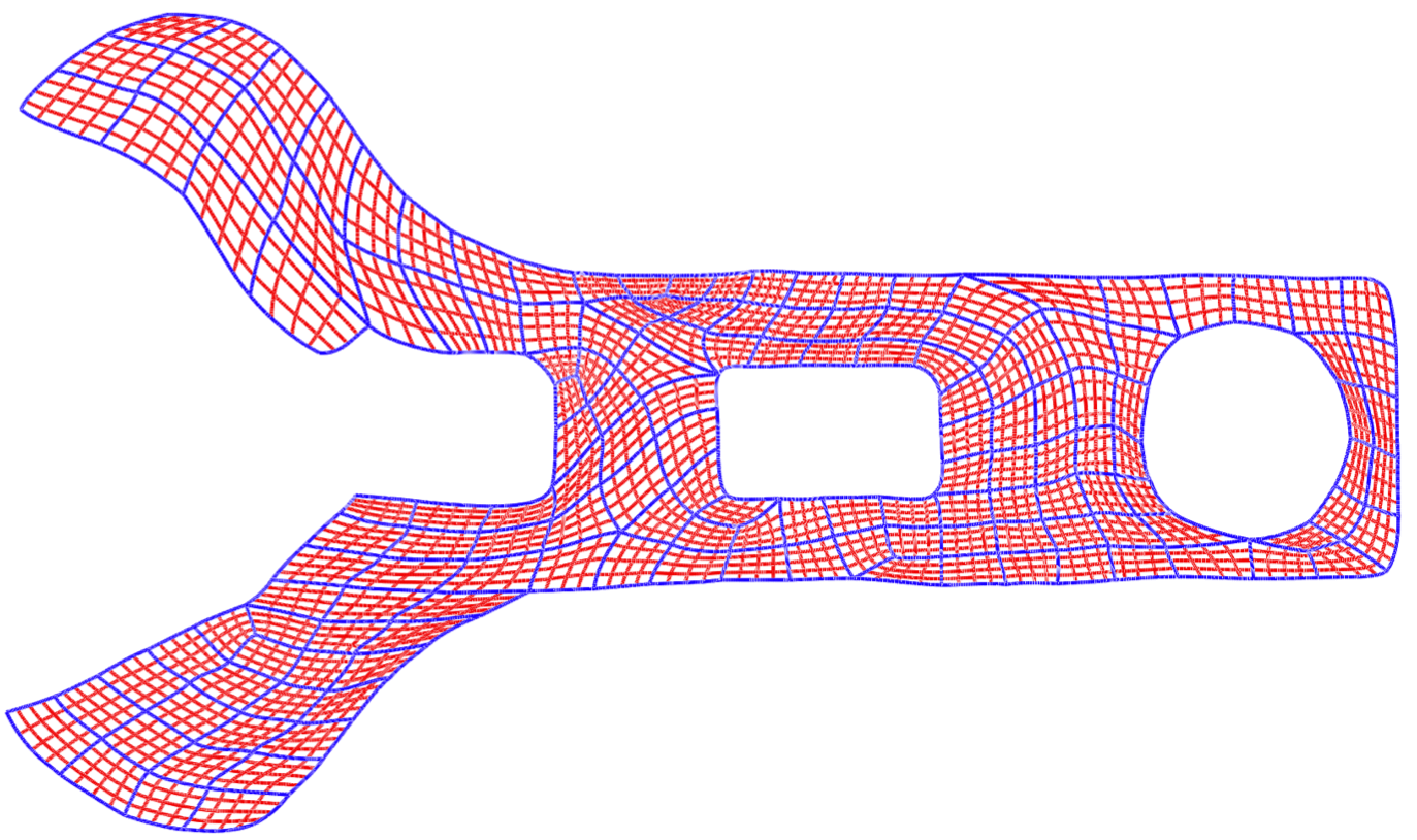
Fig. 10 (a) depicts the boundary Bézier curves after the pre-processing of input boundary B-spline curves; Fig. 10 (b) presents the discrete boundary obtained by connecting the ending control points of each Bézier curve, and the corresponding quad meshing result can be found in Fig. 10 (c). Fig. 10 (d) shows the domain partition results with the construction of segmentation curves by the global optimization method. After the local optimization for each sub-patch, the final planar parameterization is illustrated in Fig. 10 (e). The iso-parametric curves show the quality of the planar parameterization. The corresponding scaled Jacobian colormap in Fig. 10 (f) proves that the parametrization is analysis suitable. Fig. 10 (g) presents the extracted skeleton from the input boundary, Fig. 10 (h) the skeleton-based parameterization results with blue segmentation curves, and Fig. 10 (i) the corresponding scaled Jacobian colormap. More comparison examples with complex geometry can be found in Fig. 11 and Fig. 12. Since global/local optimizations with constraints are applied for the construction of segmentation curves and parameterization of Bézier subdomains, our method achieves smooth parameterizations compared to the skeleton-based approach [52].
| Example | Method | # SD | #Patch | # Con. | Scaled Jacobian | Condition number | ||||
|---|---|---|---|---|---|---|---|---|---|---|
| Average | Min | Average | Max | |||||||
| Fig. 10 | Our method | 39 | 39 | 1467 | 0.8843 | 0.292 | 2.76 | 8.06 | ||
| Xu et al.[52] | 5 | 35 | 1309 | 0.5172 | 0.148 | 5.36 | 16.31 | |||
| Fig. 11 | Our method | 66 | 66 | 1768 | 0.9194 | 0.276 | 2.42 | 10.18 | ||
| Xu et al.[52] | 8 | 56 | 1507 | 0.7801 | 0.075 | 4.35 | 18.23 | |||
| Fig. 12 | Our method | 155 | 155 | 3720 | 0.9017 | 0.294 | 2.57 | 7.86 | ||
| Xu et al.[52] | 12 | 132 | 3282 | 0.7894 | 0.134 | 4.23 | 15.64 | |||
| Example | in (14) | in (16) | in (29) | # | # | # | |||||||
|---|---|---|---|---|---|---|---|---|---|---|---|---|---|
| Fig. 1 | 2.0 | 1.0 | 2.0 | 1.0 | 50.0 | 2.0 | 1.5 | 73.22 | 177.86 | 251.08 | |||
| Fig. 9(c) | 1.0 | 1.0 | 1.0 | 1.0 | 50.0 | 1.0 | 1.5 | 22.68 | 26.64 | 49.32 | |||
| Fig. 9(g) | 1.0 | 1.0 | 1.0 | 1.0 | 50.0 | 1.0 | 1.5 | 22.96 | 27.18 | 50.14 | |||
| Fig. 9(k) | 1.0 | 1.0 | 1.0 | 1.0 | 50.0 | 1.0 | 1.5 | 27.68 | 36.32 | 63.90 | |||
| Fig. 10 | 1.0 | 2.0 | 1.0 | 2.0 | 50.0 | 1.0 | 2.0 | 32.74 | 53.84 | 86.58 | |||
| Fig. 11 | 2.0 | 1.0 | 1.0 | 2.0 | 50.0 | 2.0 | 1.0 | 41.02 | 61.36 | 102.38 | |||
| Fig. 12 | 2.0 | 1.0 | 2.0 | 2.0 | 50.0 | 2.0 | 1.0 | 75.70 | 209.68 | 285.38 | |||
Quantitative data of the comparison examples including the parameterization quality metrics with respect to scaled Jacobians and condition numbers presented in Fig. 10, Fig. 11 and Fig. 12 are summarized in Table 2. We can see from Table 2 that the proposed approach achieves analysis-suitable parameterizations with bigger average scaled Jacobians and smaller average condition numbers compared to the skeleton-based method [52]. In the comparison examples, the input boundary curves are usually B-spline curves, hence after the domain partition by skeleton-based method [52], knot-insertion operations should be performed on each sub-domain to obtain extracted Bézier patches. Although the number of subdomains in the skeleton-based method [52] is much smaller than that in our proposed method, see Table 2, the number of Bézier patches and the number of control points in the skeleton-based approach [52] are similar to those in the proposed method. These extracted Bézier patches are used as the computational elements in IGA [2].
There are several parameters involved in the objective functions of the optimization framework. Different parameterization results can be obtained from different choices of these parameters. The parameters of the objective functions in (14), in (16) and in (29) are summarized in Table 3 for the presented examples in Fig. 1, Fig. 9, Fig. 10, Fig. 11 and Fig. 12. Furthermore, the associated CPU times for the global optimization and local optimization process are listed in Table 3. The computational cost of the proposed method depends on the number of patches and the number of control points in the planar parameterization.
In conclusion, the planar parameterization obtained by the proposed global/local optimization method has high-quality, and is suitable for isogeometric applications.
8 Conclusion and future work
The parameterization of the computational domain with complex CAD boundary is a key step in IGA. In this paper, a general framework for constructing IGA-suitable planar B-spline parameterizations of the computational domain with high genus and more complex boundary curves is proposed. High-quality patch-partition results with few singularities are achieved by a global optimization method, and the Bézier patch with respect to each quad in the quadrangulation is obtained by a local optimization method yielding uniform and orthogonal iso-parametric structures while keeping the continuity conditions between patches. The proposed framework can be considered as a generalized Bézier extraction of a planar domain, and the resulting Bézier patches can be used as the computational elements for IGA [2]. The efficiency and robustness of the proposed approach are demonstrated by several examples.
In the future, we will focus on the following extensions:
- 1.
Quad mesh generation significantly influences the parameterization quality. State-of-the-art quad meshing techniques will be investigated for IGA-suitable parameterization problem.
- 2.
Several parameters are involved in the proposed optimization framework. Automatic selection of these parameters from the input data will be addressed.
- 3.
The proposed local optimization scheme can be improved by using Teichmüller mapping [29] with theoretical guarantees of injectivity, and it can be accelerated by parallelized implementation exploiting GPU/OpenMP.
- 4.
The proposed method can be extended to NURBS planar parameterization directly. Extension to three-dimensional volumetric parameterization problem with complex boundary representation will be a part of future work.
Acknowledgment
This research was supported by Zhejiang Provincial Natural Science Foundation of China under Grant Nos. LR16F020003, LQ16F020005, the National Nature Science Foundation of China under Grant Nos. 61472111, 61602138, 61502130, and the Open Project Program of the State Key Lab of CAD&CG (A1703), Zhejiang University.
Stéphane Bordas also thanks partial funding for his time provided by the European Research Council Starting Independent Research Grant (ERC Stg grant agreement No. 279578) “ RealTCut Towards real time multi-scale simulation of cutting in non-linear materials with applications to surgical simulation and computer guided surgery ”. Stéphane Bordas is also grateful for the support of the Fonds National de la Recherche Luxembourg FWO-FNR grant INTER/FWO/15/10318764.
Appendix I. Conversion of multiply-connected region
In this part, an approach for converting multiply-connected region into simply-connected region will be described.
If the region bounded by the given boundary curves is not a simply-connected region, that is, it is a multiply-connected region, we have to convert it into a simply-connected region. Suppose that the given multiply-connected region has one outer boundary and one interior boundary, then we find the vertex , such that the distance between and is minimal among all the distance between two points from the interior boundary to outer boundary. If we that is ,
| (38) |
in which is the distance between the vertex and . In order to generate a uniform quadrilateral decomposition, some extra points should be added between the vertex and . The number of added vertex is computed as follows:
| (39) |
then the added vertices between and are obtained by linear interpolation. The final boundary vertex sequence V of the simply-connected region is
| V | (40) |
For the domain with multiple components, we can apply above method iteratively, that is, in every iteration, we insert edges between the vertices that have the shortest distance between the outer and interior boundaries.
Appendix II. Proof of Proposition 6.2
Proof.
Set . The gradient of the energy functional (29) with respect to the coordinates of an unknown control points, , can be computed as follows,
From the derivatives of the Bézier surface over rectangular domain, we have
| (41) | |||
| (42) | |||
| (43) | |||
| (44) | |||
| (45) |
Hence,
| (46) | |||||
| (47) | |||||
| (48) | |||||
| (49) |
where .
References
- [1] M. Aigner, C. Heinrich, B. Jüttler, E. Pilgerstorfer, B. Simeon and A.-V. Vuong. Swept volume parametrization for isogeometric analysis. In E. Hancock and R. Martin (eds.), The Mathematics of Surfaces (MoS XIII 2009), LNCS 5654(2009) 19-44.
- [2] Michael J. Borden, Michael A. Scott, John A. Evans, Thomas J. R. Hughes. Isogeometric finite element data structures based on Bézier extraction of NURBS. International Journal for Numerical Methods in Engineering 87(1-5)(2011) 15-47.
- [3] F. Buchegger, B. Jüttler, A. Mantzaflaris. Adaptively refined multi-patch B-splines with enhanced smoothness. Applied Mathematics and Computation 272(2016) 159-172.
- [4] F. Buchegger, B. Jüttler. Planar multi-patch domain parameterizaton via patch adjacency graphs. Computer-Aided Design 82(2017) 2-12.
- [5] do Carmo, Manfredo P.. Differential geometry of curves and surfaces. Prentice Hall, 1976.
- [6] C. Chan, C. Anitescu, T. Rabczuk. Volumetric parametrization from a level set boundary representation with PHT-splines. Computer-Aided Design 82 (2017) 29-41.
- [7] E. Cohen, T. Martin, R.M. Kirby, T. Lyche and R.F. Riesenfeld, Analysis-aware modeling: understanding quality considerations in modeling for isogeometric analysis. Computer Methods in Applied Mechanics and Engineering 199(2010) 334-356.
- [8] J.A. Cottrell, T.J.R. Hughes, Y. Bazilevs. Isogeometric Analysis: Toward Integration of CAD and FEA. Wiley, 2009.
- [9] D. Den Hertog, C. Roos, T. Terlaky. On the classical logarithmic barrier function method for a class of smooth convex programming problems. Journal of Optimization Theory and Applications 73(1)(1992) 1-25.
- [10] J.M. Escobara, J.M. Cascónb, E. Rodrígueza, R. Montenegro. A new approach to solid modeling with trivariate T-spline based on mesh optimization. Computer Methods in Applied Mechanics and Engineering, 200(2011) 3210-3222.
- [11] A. Falini , J. Speh, B. Jüttler. Planar domain parameterization with THB-splines. Computer Aided Geometric Design 35-36(2015) 95-108.
- [12] A. V. Fiacco, G. P. McCormick. Nonlinear Programming: Sequential Unconstrained MinimizationTechniques. J. Wiley and Sons, New York, 1968. Reprinted as Classics in Applied Mathematics 4, SIAM, 1990. MR 39:5152.
- [13] Gravesen J, Evgrafov A, Nguyen D-M, Nørtoft P. Planar parametrization in isogeometric analysis. In: Mathematical methods for curves and surfaces. Lecture Notes in Computer Science 8177(2014) 189-212.
- [14] G. Farin. Curves and Surfaces for CAGD - A Practical Guide. 5th Edition, Morgan Kaufmann. Publishers, 2002.
- [15] T. Hermann, J. Peters, T. Strotman, A geometric constraint on curve networks suitable for smooth interpolation, Computer-Aided Design, 43(2011) 741-746
- [16] T.J.R. Hughes, J.A. Cottrell, Y. Bazilevs. Isogeometric analysis: CAD, finite elements, NURBS, exact geometry, and mesh refinement. Computer Methods in Applied Mechanics and Engineering 194(2005) 4135-4195.
- [17] M. Kapl, V. Vitrih, B. Jüttler, K. Birner. Isogeometric analysis with geometrically continuous functions on two-patch geometries. Computers & Mathematics with Applications 70(2015) 1518-1538.
- [18] M. Kapl, F. Buchegger, M. Bercovier, B. Jüttler. Isogeometric analysis with geometrically continuous functions on planar multi-patch geometries. Computer Methods in Applied Mechanics and Engineering, 316(2017) 209-234
- [19] K. Karčiauskas, J. Peters. Refinable functions on free-form surfaces. Computer Aided Geometric Design, 54(2017) 61-73.
- [20] K. Karčiauskas, T. Nguyen, and J. Peters. Generalizing bicubic splines for modelling and IGA with irregular layout. Computer Aided Design, 70(2016) 23-35.
- [21] J.M. Lien, N. M. Amato. Approximate convex decomposition of polygons. Computational Geometry 35(1-2)(2016) 100-123.
- [22] L. Liu, Y. Zhang, T. J.R. Hughes, M. A. Scott, T. W. Sederberg. Volumetric T-Spline construction Using Boolean operations. Engineering with Computers, 30(4)(2014) 425-439
- [23] X.W. Ma, G.Q Zhao, L. Sun. AUTOMESH-2D/3D: robust automatic mesh generator for metal forming simulation. Materials Research Innovations 15(1)(2011) 482-486.
- [24] T. Martin, E. Cohen, R.M. Kirby. Volumetric parameterization and trivariate B-spline fitting using harmonic functions. Computer Aided Geometric Design 26(2009) 648-664.
- [25] B. Mourrain, R. Vidunas, N. Villamizar. Dimension and bases for geometrically continuous splines on surfaces of arbitrary topology. Computer Aided Geometric Design 45(2016) 108-133.
- [26] D. Nairn, J. Peters, D. Lutterkort. Sharp, quantitative bounds on the distance between a polynomial piece and its Bézier control polygon. Computer Aided Geometric Design 16(7) (1999) 613-631.
- [27] T. Nguyen, B. Jüttler. Parameterization of contractible domains using sequences of harmonic maps. Lecture Notes in Computer Science 6920(2012) 501-514.
- [28] V.P Nguyen, P. Kerfriden, S.P.A. Bordas, T. Rabczuk. Isogeometric analysis suitable trivariate NURBS representation of composite panels with a new offset algorithm. Computer-Aided Design 55(2014) 49-63.
- [29] X. Nian, F. Chen. Planar domain parameterization for isogeometric analysis based on Teichmüller mapping. Computer Methods in Applied Mechanics and Engineering 311 (2016) 41-55.
- [30] J. Nocedal, S. J. Wright. Numerical Optimization, 2nd Edition, Springer Series in Operations Research and Financial Engineering, Springer, New York, 2006.
- [31] N. Nguyen-Thanh , K. Zhou, X. Zhuang, P. Areias , H. Nguyen-Xuan , Y. Bazilevs , T. Rabczuk. Isogeometric analysis of large-deformation thin shells using RHT-splines for multiple-patch coupling. Computer Methods in Applied Mechanics and Engineering, 316(2017) 1157-1178.
- [32] N. Nguyen-Thanh, J. Muthu , X. Zhuang , T. Rabczuk. An adaptive threedimensional RHT-spline formulation in linear elasto-statics and elasto-dynamics. Computational Mechanics, 53(2014) 369-385.
- [33] N. Nguyen-Thanh , J. Kiendl, H. Nguyen-Xuan, R. Wüchner , K.U. Bletzinger, Y. Bazilevs, T. Rabczuk. Rotation free isogeometric thin shell analysis using PHT-splines. Computer Methods in Applied Mechanics and Engineering, 200(2011) 3410-3424.
- [34] N. Nguyen-Thanh , H. Nguyen-Xuan , S. Bordas, T. Rabczuk. Isogeometric analysis using polynomial splines over hierarchical T-meshes for two-dimensional elastic solids. Computer Methods in Applied Mechanics and Engineering, 200(2011) 1892-1908.
- [35] E. Pilgerstorfer, B. Jüttler . Bounding the influence of domain parameterization and knot spacing on numerical stability in Isogeometric Analysis. Computer Methods in Applied Mechanics and Engineering 268(2014) 589-613.
- [36] Q. Pan, C. Chen, G. Xu. Isogeometric Finite Element Approximation of Minimal Surfaces Based on Extended Loop Subdivision. Journal of Computational Physics, 343(2017) 1-16.
- [37] Q. Pan, G. Xu, G. Xu, Y. Zhang. Isogeometric Analysis Based on Extended Loop’s Subdivision. Journal of Computational Physics, 299(2015) 731-746.
- [38] K.F. Pettersen, V. Skytt. Spline volume fairing. Lecture Notes in Computer Science 6920(2012) 553-561.
- [39] S.P. Sastry, S.M. Shontz, and S.A. Vavasis. A log-barrier method for mesh quality improvement and untangling. Engineering with Computers 30 (2014) 315-329.
- [40] H. Speleers, C. Manni. Optimizing domain parameterization in isogeometric analysis based on Powell-Sabin splines. Journal of Computational and Applied Mathematics 289(2015) 68-86.
- [41] K. Takayama, D. Panozzo, O. Sorkine-Hornung. Pattern-based quadrangulation for N-sided patches. Computer Graphics Forum, 33(5) (2014) 177-184.
- [42] G. Wang. Subdivision method for finding the intersection between two Bézier curves or surfaces. Journal of Zhejiang University, Special Issue on Computational Geometry (1984) 108-119.
- [43] C.C.L.Wang, K.C.Hui, K.M.Tong. Volume parameterization for design automation of customized free-form products. IEEE Transactions on Automation Science and Engineering 4 (1) (2007) 11-21.
- [44] W. Wang, Y. Zhang, L. Liu, T. J.R. Hughes. Trivariate solid T-spline construction from boundary triangulations with arbitrary genus topology. Computer-Aided Design 45(2013) 351-360.
- [45] X. Wang, X. Qian. An optimization approach for constructing trivariate B-spline solids. Computer-Aided Design 46 (2014) 179 - 191.
- [46] G. Xu, T. H. Kwok, and C. C. Wang. Isogeometric computation reuse method for complex objects with topology-consistent volumetric parameterization. Computer-Aided Design 91(2017) 1-13.
- [47] G. Xu, B. Mourrain, R. Duvigneau, A. Galligo. Optimal analysis-aware parameterization of computational domain in 3D isogeometric analysis. Computer-Aided Design 45(2013) 812-821.
- [48] G. Xu, B. Mourrain, R. Duvigneau, A. Galligo. Parameterization of computational domain in isogeometric analysis: methods and comparison. Computer Methods in Applied Mechanics and Engineering 200(2011) 2021-2031.
- [49] G. Xu, B. Mourrain, R. Duvigneau, A. Galligo. Analysis-suitable volume parameterization of multi-block computational domain in isogeometric applications. Computer-Aided Design 45(2013) 395-404.
- [50] G. Xu, B. Mourrain, R. Duvigneau, A. Galligo. Constructing analysis-suitable parameterization of computational domain from CAD boundary by variational harmonic method. Journal of Computational Physics 252(2013) 275-289.
- [51] G. Xu, B. Mourrain, A. Galligo , T. Rabczuk. High-quality construction of analysis-suitable trivariate NURBS solids by reparameterization methods. Computational Mechanics 54 (2014) 1303-1313
- [52] J. Xu, F. Chen, J. Deng. Two-dimensional domain decomposition based on skeleton computation for parameterization and isogeometric analysis. Computer Methods in Applied Mechanics and Engineering 284(2015) 541-555
- [53] Y. Zhang, W. Wang, T. J.R. Hughes. Solid T-spline construction from boundary representations for genus-zero geometry. Computer Methods in Applied Mechanics and Engineering, 201(2012) 185-197.
- [54] Y. Zhang, W. Wang, T. J.R. Hughes. Conformal solid T-spline construction from boundary T-spline representations. Computational Mechanics 51(2013) 1051-1059.