Controlling Non-reciprocity using enhanced Brillouin Scattering
Abstract
The properties of space-time modulated media operating in the sub-sonic regime are discussed based on rigorous Bloch-Floquet theory. A geometrical description in the frequency-wavenumber plane is developed to provide insight into the possible interactions and their nature. It is shown that the secular equation has a singularity, which results in a weak/passive second harmonic generation process. Additionally bandgaps arising from the strong/active parametric interaction between an incident wave and its space-time harmonic, result in an inelastic Brillouin like scattering process. Hence when the incident frequency is inside a forward (backward) bandgap, a Stokes’ (Anti-Stokes’) scattered wave bounces back to the source. Although the forward and backward bandgaps do not generally occur at the same frequency bands, the insertion loss and gap width are equal. Requiring that both gaps do not overlap, enforces a lower bound on the modulation speed. It is shown that although an increase in the modulation index is desirable, as it enhances the non-reciprocal behaviour, it also limits the range of possible modulation speeds. The effective complex refractive index is calculated over a wide frequency range. It is shown that peaks appear in the extinction coefficient, indicating scattering to Stokes’ and Anti-Stokes’ waves. Finally, a comprehensive numerical analysis based on the Finite Difference Time Domain method is developed to verify and demonstrate the intriguing properties of space-time modulated media.
I Introduction
The study of space-time modulated media sparked interest in the late 1950s and early 1960s in the exploration of the properties of travelling wave parametric amplifiers [1, 2, 3, 4, 5, 6]. In these systems, a strong wave (the pump) modulates a system parameter; for instance a varactor-loaded transmission line can be space-time modulated via the introduction of a strong pump wave that modulates the capacitance value in both space and time. A general solution of the system is determined by a wave and all its infinite space-time harmonics as dictated by the Bloch-Floquet Theorem. Traditionally whenever the modulation index is significantly small, the propagation behaviour can be explained using the parametric interaction of two waves: the signal and idler. This is equivalent to truncating the space-time harmonics expansion to two terms only. This approach, also known as three wave mixing, is widely used to describe nonlinear behaviours in optical media, such as parametric generation and inelastic scattering [7, 8]. In an early work, Slater pointed out to the common features between space-time modulated media and scattering from crystals [9]. Recently we showed that the dynamical behaviour of a sinusoidally pumped nonlinear composite right left handed transmission line (NL CRLH TL) resembles a Stimulated Brilliouin Scattering process observed in crystal structures [10, 7].
Despite the success of three wave mixing in describing scattering in nonlinear optical media, its general application to any modulated media may lead to inaccurate results. For example Oliner et al showed that, whenever the speed of modulation is close enough to the speed of the unmodulated medium (in a dispersion-less medium), the full Bloch-Floquet modes must be used [4]. They based their arguments on a rigorous mathematical framework that they developed earlier to describe wave propagation in the presence of a spatially modulated surface reactance [11]. Very recently we showed that for a NL CRLH TL, three wave mixing does not provide accurate results for strong nonlinearity and/or the TL is relatively short [12].
Quite recently there has been renewed interest in space-time modulated structures for their non-reciprocal behaviour. It has previously been shown that the dispersion relation of a medium loses its symmetry once it is space-time modulated. In this case, waves travelling in the forward and backward directions do not necessary have the same wave number (i.e , and stand for forward and backward propagation, respectively) [5]. However, such intriguing behaviour has not been exploited until recently. For instance to obtain an optical isolation in one direction, non-reciprocity was introduced via the space-time modulation of the refractive index of a photonic crystal [13]. This imparts frequency and wave number shifts during a photonic indirect interband transition. The transition is made possible in a given direction by allowing the space-time modulation to phase match the frequencies and wave number of the incident wave and a crystal mode. This is equivalent to saying that both photons energy and momentum are simultaneously conserved. By properly choosing the length of the crystal to be equal to the coherence length, efficient transfer from the incident wave to its space-time harmonic can be made possible. In the opposite direction of propagation, however, the phase matching conditions are not satisfied; hence a photonic transition does not occur and propagation is not disturbed. The non-reciprocity via inter-band transition can be induced using an electrically driven photonic crystal [14].
Using the metamaterial paradigm, space-time modulation was also exploited to introduce non-reciprocity on the meta-atomic level scale by mimicking Faraday’s rotation. This was achieved by lifting mode azimuthal degeneracy in a ring resonator via the space time modulation of the dielectric constant [15]. The modulation frequency allows the clock and anti-clock modes to resonant couple. The coupling process, analyzed by coupled mode theory [16], is mediated by the modulated dielectric constant. As a result, the coupled (hybridized) modes are different in character and as a consequence non-reciprocity arises.
In essence, the introduction of space-time modulation biases the system, leading to an asymmetric coupling of the space-time harmonics, which results in the non-reciprocal behaviour. This property was recently utilized to break time-reversal symmetry. Such property was exploited to design a multitude of interesting devices; for example: non-reciprocal leaky wave antenna [17, 18], circulators [19, 20], isolators [21] and potential novel devices such as metasurfaces [22].
In the context of an elastic media, it was shown that by properly choosing the modulation speed, a strong interaction of the space-time harmonics can be enabled; this results in the creation of a directional band-gap in one direction, while leaving propagation in the reverse direction intact [23]. The directional bandgap identifies a strong active parametric interaction [4, 5].
In the current article, we examine the properties of space-time modulated media in terms of the interaction of space-time harmonics from very low frequencies up to frequencies that correspond to the bandgaps, both in the forward and backward directions. The theoretical framework is based on the rigorous continued fraction approach [4, 5, 6]. We present a geometrical description in the plane. The detailed analysis delves into the different space-time interactions. We also show that the bandgaps are equivalent to inelastic Brillouin-like scattering centres. The insertion loss due to scattering from a modulated slab is calculated. It is shown that due to the trade-off between the modulation index and the speed of the modulation, a lower bound is enforced on the latter. Brillouin-like scattering and the active space-time harmonics in the bandgaps allow us to explain the abrupt change in the medium extinction coefficient. Finally, a detailed FDTD analysis is developed to verify and demonstrate the intriguing properties of space-time modulated media.
In section II a generalized dispersion relation is derived for an arbitrary space-time periodic medium. For subsequent discussions, the dispersion relation is simplified by considering the fundamental harmonic of the modulation wave only. The analogy to Brillouin scattering is pointed out and the scattering centres are identified. Section III describes in detail the scattering mechanism in both the forward and backward propagation directions, the width of the bandgap as well as the insertion loss in the center of the gap are also estimated; the effect of the inelastic scattering on the extinction coefficient is also demonstrated. In section IV we provide a detailed FDTD analysis to verify the theoretical analysis.
II Space-time Dispersion Relation
Here we will consider the case where the dielectric constant is modulated in both space and time as a travelling wave of the form , where is the modulation speed taken in the direction. can be expanded in terms of its Fourier harmonics
| (1) |
where and are the temporal and spatial modulation frequencies, and are related to the modulation speed as:
| (2) |
Seeking an polarised TEM solution for the wave propagating along the axis (Fig. 1), the wave equation can be written as
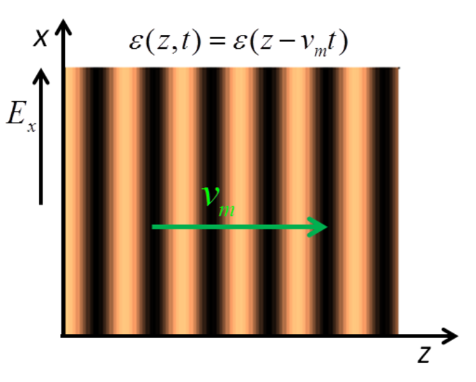
| (3) |
The disturbance in (3) is periodic in both time and space, hence we can apply Bloch-Floquet theorem to express the solution as a propagating wave modulated by a space-time periodic function ; where and are the yet to be determined frequency and wave number. The periodic function can in turn be written as an infinite Fourier series:
| (4) |
Therefore, the general solution assumes the form:
| (5) |
where the arbitrary constant is absorbed in . Substituting (5) and (1) in (3); and noting that , a recursion relation between the terms can be found to be
| (6) |
where
| (7) |
the wavelength of the modulation, is the unmodulated wave number (), is the speed of the unmodulated medium; and is the relative speed of the modulation. (6) represents an infinite system of linear algebraic equations that couple the space-time (Floquet) mode to all other modes. To find the dispersion relation for a given (), a secular (or characteristic) equation is obtained by setting the determinant of the infinitely countable system (6) to zero; hence the corresponding () can be calculated. When , . Therefore the system of equations (6) is invariant under the reflection of (), which means that if (, ) is a solution to the characteristic equation so does (, ) and the modulated medium is reciprocal. However for a general , this is not the case and the medium is intrinsically non-reciprocal.
In practical situations, the expansion (1) can be truncated to the fundamental component ( and ) only, which simplifies (6) to
| (8) |
for and
| (9) |
where is the modulation index [4]. The modulated media then couples the Floquet mode with its nearest neighbour (+1 and -1 harmonics) only.
Formally, a rigorous continued fractions approach was derived to determine the dispersion relation [4, 5]. Expressing the ratio as a continued fraction and noting that , the secular equation can be cast into the form of a continued fraction form [4, 5]
| (10) |
It is worth noting that , which means that the dispersion relation can be fully obtained from any of the infinite and they are all compatible.
For infinitesimally small , the equations (8) decouple and the dispersion relation reduces to
| (11) |
the dispersion relation of the unmodulated medium, but shifted by .
For each frequency , (10) determines the corresponding wave number . Therefore, the dispersion relation can be constructed, which is generally a function of and . However to guarantee that converges for some , it was shown that must be greater than 2; this is equivalent to saying that the modulation velocity may not be very close to the speed of waves in the unmodulated medium [4, 5]. Moreover, for stable operation (all solutions bounded in time), the sub-sonic condition or equivalently must be met. This enforces an upper bound on the modulation speed [6].
II-A Brillouin Scattering Analogy
Equation (3) establishes the formal connection between space-time modulation and Brillouin Scattering. However the analogy between the two needs more discussion. Brillouin Scattering stems from the inevitable fluctuation of thermodynamic variables, which affects the macroscopic properties of the crystal lattice. However such fluctuation is random, reciprocal and wide band [8]. Nevertheless, interaction is usually negligible except for a specific crystal mode: the one that satisfies the phase matching conditions [8, 7]. Additionally, the interaction is weak, with a very small relative speed . Space-time modulated media can then be regarded as a Stimulated or Engineered Enhanced Brillouin Scattering. Such an analogue behaviour was recently exploited to describe the interaction of a longitudinal acoustic wave with a spatio-temporal phononic crystal [24].
II-B Scattering Centres

For small values of , the dispersion relation approaches (11). Figure 2(a) depicts the dispersion relation for a space only modulation medium () and an infinitesimally small value of . Comparing this to Fig. 2(b), which depicts the dispersion relation but for , (10), reveals that the intersection points between the lines identify the loci of strong interactions. As will be shown, for a general these points allow the incident wave to scatter in an inelastic fashion and therefore will be called the Scattering Centres. The behaviour of such interactions can be studied by considering the interaction with the branches only. In the forward direction (), the intersection point of the branch and another arbitrary branch can be found to be
| (12) |
where the subscript identifies that this is the intersection with the branch and the superscript emphasises that this is for a forward propagating wave (along axis). Similarly and , the intersection with the backward branch is found to be
| (13) |
For reasons that will be revealed in Section III, we call the forward and backward scattering centres Stokes’ and Anti Stokes’ centres, respectively. For a forward propagating modulation, and hence ; the equality holds for : space only modulated medium. The inequality means that the interaction in the backward branch occurs at a lower frequency leading the medium to become non-reciprocal. Fig. 3 presents the dispersion relation for and two values of : and . It is clear that .

III Scattering Mechanism

In this section we describe the conversion (scattering) process from the fundamental wave with frequency and wave number to its space-time harmonics with frequency and wave number . The scattering behaviour depends on the values of . First, we examine the trend of as a function of the input frequency or the corresponding scaled value . Toward this end, is related to metric distances on the plane. Referring to Fig. 4, the distances , between an arbitrary point on the line and the branch of with a positive slope is
| (14) |
which is obtained by substituting the coordinate in the expression and dividing by . Similarly, the distance between and the branch of with a negative slope () is
| (15) |
Therefore,
| (16) |
The above Eq., together with Fig. 4, give a pictorial view of how depends on the geometrical metrics and . For very small values of and , and is independent of ; this means that for very low frequencies all basically have the same value. Nevertheless as increases, effect is radically different for waves travelling in the forward or backward directions, as will be detailed in the next two subsections.
III-A Forward direction ()

For a wave travelling in the direction and assuming that propagation is mainly due to the branch, , which is true for small values of and away from the bandgaps highlighted in Figs. 2(b) and 3(b). Nevertheless, the general behaviour of around the bandgaps can still be described using the approximation; for accurate results we resort to the general secular equation (10). Fig. 5 shows the change of as a function of the normalized frequency . For (), as increases along the line, linearly decreases (increases) and remains constant (refer to Fig. 4). Additionally, the denominator of (16) quadratically decreases (increases). Therefore, for , the net effect of both terms keeps monotonically decreasing.
The trend of for is more dynamic; as approaches the singularity at , increases without bound. However, as increases further, will decrease and eventually vanish at the Stokes’ centre . At this point the branch intersects the main branch (i.e, ) and the interaction is the strongest, as was already shown in Figs. 2 and 3. For such cases where attains small values, the continued fraction in (10) has to be used to determine . Otherwise, the dispersion characteristic is determined via alone, which is equivalent to the approximation used here ().
At the first singular point , the secular equation (10) reduces to
| (17) |
i.e, it depends on the interaction between the main branch and the positive space time harmonics. To find the properties and strength of this interaction, it is assumed that at , for are large enough such that their contribution to the secular equation can be ignored. This is consistent with the monotonically decreasing trend of (Fig. 5). One can then solve the truncated equation:
| (18) |
to find , evaluated at . Since is not very different from its value at , it can be approximated by
| (19) |
Neglecting orders in higher than two, the truncated characteristic equation (18) is reduced to
| (20) |
where and is always greater than one (since ). The type of the solution is determined by the radical, which for the case in hand, is always positive. Hence, is real, indicating a passive exchange of power between the wave at normalized frequency and its space-time harmonic [25]. This interaction corresponds to a weak second harmonic generation. To estimate the magnitude of the interaction (i.e, finding ), one notices that for
| (21) |
a second order in . Therefore
| (22) |
The ratio of the amplitude of the +1 harmonic and the fundamental can be determined as
| (23) |
Substituting with the typical values, , , , a very small number. Therefore, it can be concluded the the interaction between the fundamental and its +1 harmonic is very weak and can be neglected in the cases of interest. This conclusion is consistent with the dispersion relations plotted in Figs. 2(b) and 3(b), where at , the dispersion relation is basically that of the unmodulated medium.
On the other hand, the interaction at between the fundamental and its harmonic is much stronger. In general the first interaction (with the -1 harmonic) is the strongest and provides the wider bandwidth. For this reason and because it is straight forward to find closed form expressions, we will restrict our attention to the -1 harmonic interaction. At , is small (inset of Fig. 5) to the extent that the dispersion relation (10) can be truncated to
| (24) |
Letting , where , can be approximated to
| (25) |
In terms of the wave number
| (26) |
where
| (27) |
Unlike (22), is imaginary and first order in , indicating a strong active interaction [25]. The amplitude of the -1 harmonic can be found to be
| (28) |
which, unlike (23), does not depend on .
The general solution can be written as follows [3]
| (29) |
where
| (30) |
Please note that the above general solution assumes that the contributions from other branches are ignored (ignoring the multi-valued character of ). Noting that [3]
| (31) |
the characteristic impedances of the space-time medium at frequencies and are
| (32) |
and
| (33) |
respectively, and is the impedance of the unmodulated medium.
According to (31), the fundamental and scattered waves have phase velocities which are equal in magnitude but opposite in direction. Moreover, the sign of is negative implying that the scattered wave is travelling in the direction. This is consistent with Coupled Mode Theory predictions where active interaction is possible between waves which have the same magnitude of phase velocity and energy flow is contra-directive [26]. Additionally, the phase matching conditions automatically emerge:
| (34) | |||
| (35) |
Since the scattered wave is red-shifted (lower in frequency), it corresponds to a Stokes’ wave, which explains why the scattering centre was named Stokes’ centre earlier in Section II.
Considering the situation depicted in Fig. 6, where a wave of frequency impinges the modulated medium of length . The tangential fields and are continuous at the interfaces and . Approximating the impedance of the fundamental and +1 harmonic to and , respectively as shown in the Fig., the amplitude of the transmitted wave is found to be
| (36) |
and the total attenuation, ATT, of the modulated medium in Nepers is
| (37) |
which reveals interesting conclusions. As expected the attenuation is directly proportional to , but decreases as the modulation speed increases. It is then desirable to make as small as possible. However, as will be shown in the subsection C, has a lower bound determined by non-reciprocity. Additionally, from (37) the attenuation is proportional to the normalized length of the medium (normalized to the modulation wavelength); hence suggesting that to have an efficient scattering the modulation wavelength should be as small as possible. However, this might be constrained by the lower or upper bound of .

III-B Backward Direction ()
For the backward propagation , the values along the line assume the form
| (38) |
Fig. 7 shows how changes as a function of the input frequency. Although the trend in Fig. 7 look similar to Fig. 5, there are some fundamental differences which do not allow the backward propagation to be treated as the mere dual of the forward one. First, for the forward propagation, at the singularity the interaction is with the harmonics only. As a result, it was shown in the previous subsection that the +1 harmonic interacts passively with the fundamental. Additionally, it is not possible to position the singularity at the Stokes’ scattering centre . However for backward propagation, the singularity is still at . Additionally, choosing positions the singularity at the Anti-Stokes’ centre, hence limiting the scattering to be strictly with the harmonics only.

Similar to the analysis of the previous subsection, the truncated secular equation
| (39) |
can be solved to find the propagation constant at . Neglecting terms of order higher than , is found to be
| (40) |
identical to (25). In terms of the wave numbers
| (41) |
where
| (42) |
Similarly,
| (43) |
For small values of , Fig. 8 shows the situation where the modulated medium is impinged by a wave at frequency . It is worth to notice that the two situations depicted in Figs. 6 and 8 represent waves which have different frequencies. In the forward direction the wave is at a normalized frequency , while in the backward direction its normalized frequency is .
The backward attenuation takes a form identical to (37), but at a normalized frequency of . This means that by the proper selection of and the medium acts as non-reciprocal bandstop filter, where the forward and backward stop bands can occur at different frequency ranges.
The scattered wave is an Anti-Stokes wave and the interaction automatically satisfies the phase matching conditions
| (44) | |||
| (45) |

III-C Width of Directional Bandgap
The width of the directional bandgap determines the bandwidth at which the medium exhibits strong non-reciprocity. It also sets the lower bound on the modulation speed . To demonstrate non-reciprocity in one direction only, the forward and backward bandgaps must not overlap. Hence
| (46) |
where and are the directional bandgaps in the forward and backward directions, respectively. At the band edges (Fig. 9). Substituting these values in the corresponding secular equations (24) and (39), it can be found that to second order:
| (47) |
Therefore, the minimum value of is determined from the inequality (46) to be
| (48) |
which is identical to the value determined in [23] for modulated elastic media. Therefore for optimum non-reciprocal behaviour
| (49) |

III-D Complex Refractive Index,
At an arbitrary incident frequency , the complex wavevector can be written as
| (50) |
where is the complex refractive index. The imaginary part determines the efficiency of the power scattered by the space-time harmonics (forward: , backward ). Using the dispersion relation (10), the refractive index is calculated for the forward and backward directions as shown in Fig. 10. For the calculations, 20 terms were used to compute the continued fractions; usually four of five terms are enough, as the continued fractions rapidly converge.
From Fig. 10, it is clear that the optical property of the medium is non-reciprocal; absorption occurs at different input frequencies. Additionally, the widths of the Stokes and Anti Stokes Centres are basically the same because as was already determined in the previous subsection.

IV FDTD Analysis
The space-time dependence of the permittivity was used to modify the update equations of the FDTD formalism to determine the propagation and scattering behaviour of a space-time modulated medium. For more details on the FDTD implementation please refer to the Appendix. Fig. 11(a) presents the scenario where and the modulation travels in the direction, In this case, the incident wave interacts with its +1 harmonic, which scatters energy back in the direction, as is clear after inspecting the frequency spectrum of the scattered field. At this point, the scattered wave is the Anti-Stokes’ wave in Brillouin Scattering. However if the modulation speed was inverted as in Fig. 11(b), the modulation and incident waves are co-directional. In this case, as shown in Fig. 11(b), propagation is not disturbed and the medium is transparent. Hence, the medium is non-reciprocal at , in agreement with the analytical predictions.

To demonstrate that scattering occurs only inside the band gap, Fig. 12 depicts three different situations, where the FDTD algorithm was used to determine the wave propagation behaviour for an input wave of , and , when and . The first and last frequencies are outside the bandgap. As expected, strong Brillouin-like scattering occurs when only. For the other two out-of-band frequencies ( and ) the medium is transparent, demonstrated by 0 dB in the transmission spectra in Figs. 12(a) and (c).

According to Eqs. 42 and 41, the field at is actively converted to the one at . To demonstrate this, Fig. 13 presents the fields calculated at both frequencies. These plots are determined from the FDTD computations, after applying Fourier transform. The plots do indeed verify that the conversion is exponential; the incident fields are scattered into the frequency (blue-shifted), which bounces back to the source. Additionally, the envelopes of the two waves, determined from 42, 41 and 43 match the FDTD calculations.

As discussed earlier, the modulation results in a bandgap, where scattering is the strongest at the centre of the gap and decreases until it eventually becomes zero at the band edges. In Fig. 14 we plot the FDTD calculated insertion loss for different input frequencies inside the gap, superimposed on the dispersion characteristics determined by (10). As Fig. 14 shows, the insertion loss is maximum at the centre of the bandgap and becomes negligibly small at the band edges.

V Conclusion
A systematic analysis of the harmonics interactions present in a space-time modulated medium is carried out over a frequency range which extends from DC up to around the bandgaps in both the forward and backward directions. It is demonstrated that a passive second harmonic generation process does occur due to the singularity in the secular equation. However such behaviour is very weak and can be ignored. On the other hand, bandgaps in the forward and backward directions are created due to the active parametric interaction of an incident wave with its space-time harmonics. In this regime, the interaction can be described using a Brilliouin-like scattering process. The strength of scattering from a bandgap as well as its width were determined. To have an optimal full non-reciprocal behaviour, the modulation speed may not be below a certain threshold which is a function of the modulation index. Finally FDTD was used to verify the theoretical results and findings.
[FDTD Implementation]

As depicted in Fig. 15, the medium is excited by an incident wave travelling in the direction, which is applied at a Total Field/Scattered Field (TF/SF) interface [27, 28]. To the right of the interface is the total field region. The grid is terminated from both sides by absorbing boundaries. The electric and magnetic fields are polarized in the and directions, respectively to guarantee that the wave propagates in the direction. Taking into account the space time variation of the dielectric constant , the FDTD discretized form of Ampere’s law can be written in terms of Courant number (where and are the discretized spatial and temporal step, respectively) as:
Here the superscript and subscript indicate the time and spatial steps, respectively; is the impedance of free space, and is the relative permittivity at grid point at time . The update equation of the magnetic field is obtained via the discretization of Faraday’s law:
The TF/SF plane is positioned between an H and E nodes. Hence the update equation for the H node at and E node at are amended by the following equations[27]
where is the electric field of the incident wave, and are its frequency and wave number, respectively. In the above eqns., the incident electric field is referenced to the position (i.e, ).
References
- [1] P. Tien, “Parametric amplification and frequency mixing in propagating circuits,” Journal of Applied Physics, vol. 29, no. 9, pp. 1347–1357, 1958.
- [2] A. Cullen, “A travelling-wave parametric amplifier,” Nature, vol. 181, no. 4605, pp. 332–332, 1958.
- [3] J.-C. Simon, “Action of a progressive disturbance on a guided electromagnetic wave,” IRE Transactions on Microwave Theory and Techniques, vol. 8, no. 1, pp. 18–29, 1960.
- [4] A. A. Oliner and A. Hessel, “Wave propagation in a medium with a progressive sinusoidal disturbance,” IRE Transactions on Microwave Theory and Techniques, vol. 9, no. 4, pp. 337–343, July 1961.
- [5] E. S. Cassedy and A. A. Oliner, “Dispersion relations in time-space periodic media: Part i; stable interactions,” Proceedings of the IEEE, vol. 51, no. 10, pp. 1342–1359, Oct 1963.
- [6] E. S. Cassedy, “Dispersion relations in time-space periodic media part ii; unstable interactions,” Proceedings of the IEEE, vol. 55, no. 7, pp. 1154–1168, July 1967.
- [7] R. W. Boyd, Nonlinear optics, 3rd ed. Boston: Boston : Academic Press, 2008, includes bibliographical references and index.
- [8] I. L. Fabelinskii, Molecular scattering of light. Springer Science & Business Media, 2012.
- [9] J. C. Slater, “Interaction of waves in crystals,” Reviews of Modern Physics, vol. 30, no. 1, p. 197, 1958.
- [10] S. Y. Elnaggar and G. N. Milford, “Description and stability analysis of nonlinear transmission line type metamaterials using nonlinear dynamics theory,” Journal of Applied Physics, vol. 121, no. 12, p. 124902, 2017.
- [11] A. Oliner and A. Hessel, “Guided waves on sinusoidally-modulated reactance surfaces,” IRE Transactions on Antennas and Propagation, vol. 7, no. 5, pp. 201–208, 1959.
- [12] S. Elnaggar and G. Milford, “Three wave mixing as the limit of nonlinear dynamics theory for nonlinear transmission line type metamaterials,” IEEE Transactions on Antennas and Propagation, Under review.
- [13] Z. Yu and S. Fan, “Complete optical isolation created by indirect interband photonic transitions,” Nat Photon, vol. 3, no. 2, pp. 91–94, 2009, 10.1038/nphoton.2008.273.
- [14] H. Lira, Z. Yu, S. Fan, and M. Lipson, “Electrically driven nonreciprocity induced by interband photonic transition on a silicon chip,” Phys. Rev. Lett., vol. 109, p. 033901, Jul 2012.
- [15] D. L. Sounas, C. Caloz, and A. Alù, “Giant non-reciprocity at the subwavelength scale using angular momentum-biased metamaterials,” Nature Communications, vol. 4, p. 2407, 2013.
- [16] J. N. Winn, S. Fan, J. D. Joannopoulos, and E. P. Ippen, “Interband transitions in photonic crystals,” Phys. Rev. B, vol. 59, pp. 1551–1554, Jan 1999.
- [17] Y. Hadad, J. C. Soric, and A. Alu, “Breaking temporal symmetries for emission and absorption,” Proceedings of the National Academy of Sciences, vol. 113, no. 13, pp. 3471–3475, 2016.
- [18] S. Taravati and C. Caloz, “Mixer-duplexer-antenna leaky-wave system based on periodic space-time modulation,” IEEE Transactions on Antennas and Propagation, vol. 65, no. 2, pp. 442–452, 2017.
- [19] S. Qin, Q. Xu, and Y. E. Wang, “Nonreciprocal components with distributedly modulated capacitors,” IEEE Transactions on Microwave Theory and Techniques, vol. 62, no. 10, pp. 2260–2272, 2014.
- [20] N. A. Estep, D. L. Sounas, and A. Alù, “Magnetless microwave circulators based on spatiotemporally modulated rings of coupled resonators,” IEEE Transactions on Microwave Theory and Techniques, vol. 64, no. 2, pp. 502–518, 2016.
- [21] S. Taravati, N. Chamanara, and C. Caloz, “Nonreciprocal electromagnetic scattering from a periodically space-time modulated slab and application to a quasi-sonic isolator,” arXiv:1705.06311, 2017.
- [22] C. Caloz, K. Achouri, Y. Vahabzadeh, and N. Chamanara, “Spacetime metasurfaces,” in 2016 Photonics North (PN), May 2016, pp. 1–2.
- [23] G. Trainiti and M. Ruzzene, “Non-reciprocal elastic wave propagation in spatiotemporal periodic structures,” New Journal of Physics, vol. 18, no. 8, p. 083047, 2016.
- [24] C. Croënne, J. Vasseur, O. Bou Matar, M.-F. Ponge, P. Deymier, A.-C. Hladky-Hennion, and B. Dubus, “Brillouin scattering-like effect and non-reciprocal propagation of elastic waves due to spatio-temporal modulation of electrical boundary conditions in piezoelectric media,” Applied Physics Letters, vol. 110, no. 6, p. 061901, 2017.
- [25] W. H. Louisell. New York, Wiley, 1960, (William Henry).
- [26] J. R. Pierce, “Coupling of modes of propagation,” Journal of Applied Physics, vol. 25, no. 2, 1954.
- [27] J. B. Schneider, “Understanding the finite-difference time-domain method,” School of electrical engineering and computer science Washington State University.–URL: http://www. Eecs. Wsu. Edu/˜ schneidj/ufdtd/(request data: 29.11. 2012), 2010.
- [28] A. Taflove and S. C. Hagness, Computational electrodynamics. Artech house publishers, 2000.