Microlensing of Extremely Magnified Stars near Caustics of Galaxy Clusters
Abstract
Recent observations of lensed galaxies at cosmological distances have detected individual stars that are extremely magnified when crossing the caustics of lensing clusters. In idealized cluster lenses with smooth mass distributions, two images of a star of radius approaching a caustic brighten as and reach a peak magnification before merging on the critical curve. We show that a mass fraction () in microlenses inevitably disrupts the smooth caustic into a network of corrugated microcaustics, and produces light curves with numerous peaks. Using analytical calculations and numerical simulations, we derive the characteristic width of the network, caustic-crossing frequencies, and peak magnifications. For the lens parameters of a recent detection and a population of intracluster stars with , we find a source-plane width of for the caustic network, which spans on the image plane. A source star takes years to cross this width, with a total of crossings, each one lasting for with typical peak magnifications of . The exquisite sensitivity of caustic-crossing events to the granularity of the lens-mass distribution makes them ideal probes of dark matter components, such as compact halo objects and ultralight axion dark matter.
Keywords:
gravitational lensing: strong, gravitational lensing: micro, galaxies: clusters: general=2
I Introduction
Galaxy clusters are the largest gravitational lenses that can make multiple images of, and substantially magnify, sources at cosmological distances. Clusters with smoothly distributed surface mass densities have critical curves with angular sizes of tens of arcseconds on their image planes, where the lensing magnification formally diverges; these curves map to caustic curves on the source plane [3]. Background galaxies that lie on caustics appear as giant arcs, made up of two images of the part of the source inside the fold [19, see e.g.]. When a member star crosses from the inside of the caustic to the outside, a pair of images approach the critical curve from both sides, brighten to a peak magnification, and eventually merge and disappear [53]. Due to the extreme magnifications involved, single stars at high redshifts can become detectable by current telescopes. Recently, a candidate caustic-crossing event was reported in Hubble Space Telescope (HST) observations of the cluster lens MACS J1149.5+2223 [42]. Fig. 1 shows the magnification maps of the cluster for a source at redshift , computed using publicly available lens models.
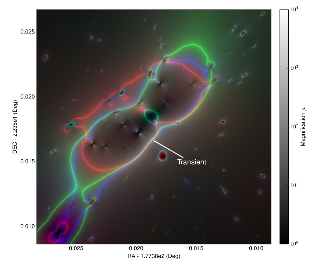
Three physical effects limit the peak magnification of a source during a caustic-crossing event. The first is the finite angular size of the source. The length of a lensed image is inversely proportional to the square root of the separation between the source and the fold caustic. Since gravitational lensing conserves the surface brightness, this implies that the peak magnification [65]. The second limitation is the effect of wave diffraction. If the physical size of a lensed image is smaller than the geometric mean of the wavelength and the distance to the lens, diffraction reduces the peak magnification [56]. We will see that this second limitation is unimportant in our situation of interest. The third limitation is the underlying granularity of the surface mass density due to the presence of discrete microlenses. When the source approaches the caustic of the smooth mass distribution, even a tiny mass fraction in microlenses substantially perturbs the lens model. The microlenses disrupt the macrocaustic into a network of corrugated microcaustics, whose characteristic peak magnifications are reduced compared to that of the smooth model [70, 4].
An example of a population of microlenses is intracluster stars. First postulated by [78] based on observations of the Coma Cluster, the presence of an intracluster stellar population has been supported by the discovery of planetary nebulae [2, 15], red giant stars [26], and supernovae [27] in intracluster space. Deep exposures of intracluster light in typical galaxy clusters have revealed smooth halos containing as much as of all the stars in their inner regions [46, 76]. Their origin may be explained by tidal stripping of cluster galaxies or by in-situ formation in intracluster clouds, which may themselves have been tidally ejected from galaxies [48, 16, 17].
In this paper, we study the characteristics of microcaustic networks produced by intracluster stars in the vicinity of the critical curves of galaxy clusters. We derive the typical angular extent of the networks, both on the image and source planes. Sources crossing these networks exhibit numerous magnification peaks as they cross microcaustics. We derive the typical peak magnification and peak frequency within the network, and demonstrate how the source intermittently brightens and becomes visible over periods of years. Due to the extreme background magnification, the associated microcaustic-crossing frequency is orders of magnitude higher than that in quasar microlensing ([14]; see [63] for a detailed review). The network of corrugated caustics, and the resultant light curves of the crossing sources, is sensitive to extremely small mass fractions of microlenses. Concomitantly, these lensing systems are sensitive to fluctuations of small amplitude in the mass density on small scales and are powerful probes of the granularity of the mass distribution in galaxy clusters.
We therefore extend our analysis and examine the possibility that the dark matter in cluster halos is partly composed of compact objects, usually called MAssive Compact Halo Objects (MACHOs), which could be primordial black holes formed in the early universe [57, 29]. Constraints on the fraction of dark matter in MACHOs have been derived using galactic microlensing [1], microlensing toward the Magellanic Clouds and M31 [68, 54], wide binaries [13, 74, 60], microlensing of the Kepler stars [31, 30], and stellar cluster dynamics [7]. In combination, these constraints rule out the possibility that MACHOs account for all the dark matter, except within a few mass windows [11]. However, the possibility remains that MACHOs comprise a small fraction of the dark matter. We discuss how this population would qualitatively modify microlensing light curves during crossings of the caustic network and show that a small fraction of dark matter in MACHOs can be probed with a sensitivity that has so far not been achieved with other existing methods.
We begin in Sec. II by reviewing the theory of caustic crossings in smooth lens models and developing simple analytic estimates of the relevant scales after including microlenses. Next, we compare these analytic results to numerical simulations of the light curves in Sec. III, for small stellar surface mass densities, following which we extrapolate the results to the realistic surface mass densities inferred from existing observations. We then discuss the effect of MACHOs in Sec. IV. We finish with some concluding remarks in Sec. V. We provide a technical calculation for the mean magnification through caustic crossings in App. A. We estimate in App. B the surface mass density in intracluster stars in the specific case of a candidate caustic-crossing event in the galaxy cluster MACS J1149.5+2223. Throughout this paper, we assume the Planck best-fit CDM cosmology with and [58].
II Structure of a corrugated caustic network: analytic estimates
II.1 Caustics in smooth lens models: definitions and notation
We first consider the vicinity of a caustic in a smooth lens model, in the absence of microlensing by point masses. In the region of geometrical optics and under the thin lens approximation, lensing is described by a mapping from the two-dimensional angular coordinates on the image plane onto the coordinates on the source plane, of the form . Here, is the two-dimensional gradient with respect to the coordinates , and the projected gravitational potential is determined by the smooth mass density projected on the image plane, or surface mass density , according to [3, e.g.,]
| (1) |
Here, is the critical surface density, and in a Friedman-Robertson-Walker universe, , , and are the angular diameter distances to the lens, to the source, and from the lens to the source, respectively. The quantity is called the convergence. Each point on the image-plane maps to a unique point on the source plane, but not vice versa—a given source can have more than one image. A smooth lens produces multiple images of sources that are within regions bounded by caustic curves on the source plane. Whenever the source crosses these caustics, multiple images annihilate or emerge in pairs on critical curves on the image plane.
The Jacobian matrix of the lens mapping takes the following form
The convergence is determined by the local surface density according to Eq. (1), while the shear is governed by the tidal force from the entire mass distribution. The inverse determinant of the Jacobian matrix is the magnification of an image at position , i.e., .
The magnification formally diverges at critical curves on the image plane (which map to caustics on the source plane), so these curves are the loci of the equation [3]. They are typically located in regions where is of order unity. We designate the characteristic angular size of the critical curves by . In the simplest model of a cluster lens as a singular isothermal sphere, this angular size is the Einstein angular radius,
| (5) |
where is the velocity dispersion of the isothermal sphere.
The region of interest in this paper is in the immediate vicinity of a critical curve, where the image magnification is very large. It is convenient to expand the components of the Jacobian matrix of Eq. (II.1) in a coordinate system centered at one chosen point on the critical curve and oriented according to the principal directions, so that is diagonal and its first eigenvalue vanishes. We then have and . The first-order expansion near the origin is
| (6) | |||||
| (7) | |||||
| (8) |
where the sub-indices indicate quantities computed at . The inverse magnification is
| (9) | ||||
| (10) |
where the vector is the gradient of the eigenvalue that vanishes at the origin. To first order, the critical curve is locally given by the straight line , i.e. it is perpendicular to the vector . Fig. 2 depicts this geometry: the critical curve is at an angle relative to the first axis, along which images are elongated into “arcs” on the image plane. This angle is , where the sub-indices and denote Cartesian components along the first and second axes, respectively. On the source plane, the caustic is a parabola crossing the origin and tangent to the second axis.
Consider a point source at a separation from the caustic in Fig. 2. When , the source has two images of equal (absolute) magnification but opposite parity, located symmetrically on both sides of the critical curve and elongated along the direction. The two images have an angular separation
| (11) |
where is the modulus of the vector . The total magnification of the two images, , is
| (12) |
In this equation, the quantity is usually of order unity and the gradient is of the order . The angle can be very small for a nearly spherically symmetric lens or when the fold is close to being a cusp.11 1 A cusp is a special point along the caustic and critical line where the angle , for which a higher-order expansion is required to analyze the variation of the Jacobian matrix in its vicinity on the image plane. In most cases, when images are not very close to a cusp, their magnification is of order . The source size, , limits the maximum magnification, which is reached when .
If the source moves relative to the lens from the inside of the caustic to the outside, two of its images move toward each other along the axis (irrespective of the direction of the source motion, as long as it is not exactly parallel to the caustic), and gradually brighten until they merge on the critical curve and disappear. The reverse process occurs when the source moves from the outside to the inside of the caustic curve. The total magnification follows a power law with the time to image merger
| (13) | |||||
where is the proper time measured by the observer and is the time of the caustic crossing. Here, we use fiducial values for the distances appropriate for the case of the gravitational lens MACS J1149+2223, at redshift , with a lensed galaxy at redshift , as we describe in more detail in App. B [42, see]). We note that the low value of inferred for the position of the observed transient in this cluster helps achieve a high magnification. The velocity is the difference in the proper velocities of the background source () and the smooth lens () with respect to the Earth, appropriately redshifted and projected along the direction perpendicular to the caustic,
| (14) |
where and are the source redshift and the lens redshift, respectively, and is a unit vector on the source plane perpendicular to the caustic (on the image plane, is also the direction of image elongation; it points along the first coordinate axis in the coordinate system of Fig. 2). With this scaling, the velocity measures the physical displacement at the source redshift per unit observer proper time; the fiducial value reflects the typical motion of the large-scale structure.
In Eq. (13), the net magnification of the pair of images formally diverges for a point source that is exactly on the caustic. As we have mentioned in the introduction, in reality, in the absence of microlenses, two effects physically limit the maximum magnification at the time of caustic crossing. They are the finite size of the source and wave diffraction. The diffraction limit is roughly [18, see, e.g.,]
| (15) |
where is the wave frequency and is the lens redshift. If we ignore the wave effects, a uniform disk source with physical radius reaches a maximum magnification [53]
| (16) |
where is the solar radius. For observations of cluster lenses at cosmological distances at optical or near-infrared wavelengths, , and thus diffraction effects are unimportant even for stars as small as white dwarfs. The duration of the magnification peak (in the observer frame) is roughly the time it takes for the stellar disk to traverse the caustic,
| (17) |
Since a star of solar luminosity at redshift has an apparent magnitude , a star with magnified by a factor of would become visible to HST at magnitude during one of these caustic crossings. However, as we shall show next, the caustic-crossing peak magnification is actually much lower than this simple estimate due to the presence of microlenses in the intracluster region.
II.2 Caustic crossing with microlenses
In this section, we use simple analytical scaling arguments to demonstrate how point masses, such as stars, in the vicinity of a macroscopic lens model critical curve transform the macrocaustic curves (with only a few cusps) into a network, or band, of corrugated microcaustics. We show how this systematically reduces the peak magnification, so that stars of higher luminosity, , are needed to make caustic-crossing events visible to current telescopes at magnitude . At the same time, each star crosses a very large number of microcaustics as it moves relative to the foreground lens across the network, so that the rate at which caustic crossings occur is greatly enhanced. We estimate the characteristic mean and peak magnifications and time-scales of the resulting light curves.
We model a cluster lens as a smooth mass distribution (in the sense of coarse-graining) with critical curves of characteristic angular size , and a total projected mass within, but with part of this mass actually in the form of point masses. In App. B, we estimate the contribution of intracluster stars to the convergence near the critical curves to be , for the cluster lens shown in Fig. 1.
It is worth pausing to clarify an issue of nomenclature in order to avoid confusion in what follows. In order to numerically study the impact of microlenses, we restrict them to a circular region of radius on the image plane, within which we distribute them randomly (the size is large enough to ignore the influence of microlenses outside the region, except near the edges that are not used). A given lens model in the literature has a surface mass density due to an entirely smooth component. We refer to this as “the macroscopic lens model,” or simply “the macroscopic model,” and we use the subscript M for the associated quantities. When including point masses with an average surface mass density within , we also appropriately reduce the smooth component to preserve the total mass. We use the term “the smooth lens model,” or simply “the smooth model,” and the subscript S, to refer to the smooth component of the model with a surface mass density , without any microlens. This is distinct from the model we start with, i.e., the macroscopic lens model with the fully smooth surface density . Both models have the same shear within the region . However, they have different critical curves on the image plane—we use the term “the smooth critical curve” for the smooth lens model and the term “the macrocritical curve” for the macroscopic lens model. We refer to the caustic of the latter lens model as the “macrocaustic”.
II.2.1 The band of corrugated microcritical curves
Consider a point microlens with mass , located close to the smooth critical curve on the image plane. We use the same notation as in Fig. 2 (which we take to represent the smooth model), in which the coordinate origin lies on the smooth critical curve that is inclined at an angle with respect to the axis of image elongation , and the coordinate represents the angular displacement from this curve.
In the absence of the smooth lens, the characteristic size of the microcritical curve is the point-mass Einstein radius
| (18) |
We first study the case of a small surface density in point masses, so that we can neglect the influence of nearby microlenses on microcritical curves near a point mass. In this case, we can approximate the Jacobian matrix as the sum of the contributions of the smoothly distributed mass, and a single point mass. We can make two further approximations in the vicinity of the smooth critical curve: first, the eigenvalue for the smooth lens model, which holds when the separation ; second, the microcritical curve around the point mass is much larger in size than the Einstein radius of Eq. (18). We will see that the latter results from the large magnification of the smooth lens model in the vicinity of its critical curve. Consequently, the separation between the microcritical curve and the point mass is typically much larger than the angular scale . Under these two assumptions, we can neglect the shear component due to the point mass and compute the magnification using , where the shear includes the contribution of the point mass. The critical curve satisfies
| (19) |
The solution to Eq. (19) consists of two branches. One branch is the original smooth critical curve (), with a perturbation that is largest at the closest distance to the point mass. The second, dumbbell-shaped, branch is in the vicinity of the point mass; the dumbbell aligns with the principal axes of the shear defined by the smooth lens and changes orientation for point masses inside or outside the smooth critical curve. This can be seen in Fig. 3, which shows critical curves that have been calculated exactly when a point mass is located at various distances to the smooth critical curve and are well-approximated by Eq. (19).
The dumbbell-shaped critical curves have a characteristic size
| (20) |
Closed critical curves near microlenses are generic when external shear breaks circular symmetry [14, 64]. When the magnification of the smooth model is very large, the area of the closed critical curve, and hence the microlensing cross-section, is greatly increased. Note that these curves never pass through the point mass, and they are actually closed and differentiable (Eq. (19) is no longer valid very near the point mass), even though this is not apparent at the resolution of Fig. 3.
When the point mass is close enough to the critical curve, i.e., when the separation , the two branches merge. We solve for this separation by substituting in Eq. (20):
| (21) |
Fig. 3 shows the behavior of both branches of the perturbed critical curve as the microlens is brought successively closer to the smooth critical curve.
This characteristic separation, at which critical curves around a single point mass merge with the ones in the smooth lens model, defines a threshold surface mass density :
| (22) |
Physically, at this surface mass density, a large portion of the smooth critical curve is strongly perturbed and merges with the ones around nearby point masses, which in turn strongly interact with each other in this region. The threshold value increases with the microlens mass as .
If the surface mass density in point masses is below the threshold value, i.e., , the smooth critical curve is not highly perturbed except over a small fraction of its length. We see from Eq. (22) that the value of is numerically small for the fiducial mass scale associated with microlensing by ordinary stars in a typical cluster lens. Thus, reasonable densities of intracluster stars can easily satisfy . In this case, the smooth critical curve is strongly perturbed everywhere and forms a network due to the combined shear of many microlenses. We can analytically estimate the general properties of this network, or band, of corrugated microcritical curves. For simplicity, we assume that (a) all microlenses have the same mass , and therefore identical angular Einstein radius , and (b) the average surface mass density in point masses is uniform in the vicinity of the smooth critical curve (up to Poissonian fluctuations). As noted earlier, the smooth component contributes the remaining surface mass density, .
The typical separation between neighboring point masses is
| (23) |
Near the smooth critical curve, the microcritical curves of point masses merge with those of the neighboring masses, and form a band extending out to a distance . We can estimate this distance by equating the microcritical curve size from Eq. (20) to the interlens separation from Eq. (23). This yields the estimate
| (24) |
This length scale has a simple physical interpretation: it is the scale at which the eigenvalue (which determines the magnification) typically receives comparable contributions from the smooth component and from the microlenses.
Fig. 4 shows an example of critical curves on the image plane, and the thickness of the critical curve network, for a population of microlenses with . The underlying macroscopic model is that of Fig. 1 at the location of the transient, but brought to the orientation of Fig. 2 with an extra rotation. The critical curves shown are exactly calculated as contours of the condition . The solid line shows the smooth critical curve, and the dashed lines show the edges of the network, as discussed above. Note that one edge of the band (the short-dashed line in the figure) is the critical curve of the macroscopic lens model, i.e., the model without microlenses and with the convergence contribution not removed from the region . Note also that the figure is centered on this macrocritical curve instead of on the one for the smooth lens model (the solid line).
We observe that outside the band of total width , the critical curves typically form loops associated with only one or a few point masses, while inside the band the loops are either larger or join the corrugated network of critical curves that separates regions with two different signs of the eigenvalue . This figure confirms our expectation, from our analytic derivation, for the width of the band of corrugated critical curves.

II.2.2 The band of corrugated microcaustics: total width and peak magnifications
We now consider the statistics of microcaustic crossings on the source plane. Throughout, we use the coordinate system of Fig. 4, with the origin on the macroscopic critical curve (and not the one for the smooth model).
We first compute the width, , of the band of corrugated caustics on the source plane. This band is the result of mapping the network of microcritical curves of Fig. 4 onto the source plane. We assume that the stochastic deflection from all point masses is small compared to the width ; we will check the validity of this assumption later. We can then use the lens map of the macroscopic lens model to relate the widths of the networks on the image and source planes. We therefore use Eq. (11) to find the source displacement needed to create an image at position at the edge of the corrugated band, as seen in Fig. 4), to obtain
| (25) |
where the factor dividing accounts for the fact that the band of corrugated critical curves is inclined at an angle to the direction of large magnification (the horizontal direction in Fig. 4).
Fig. 5 shows the microcaustic network on the source plane for the lens map of Fig. 4. The caustics are exactly obtained by mapping the critical curves to the source plane under the lens map. The source generating the blue images in Fig. 4) is the red circle in the lower panels. The rightmost dashed red line defines the boundary of the caustic network of width .

A source traversing this band will show many magnification peaks, corresponding to the crossing of multiple microcaustics. This entire set of peaks occur over a time
| (26) |
We can estimate the total number of microcaustic crossings over the time by assuming that there is typically one critical curve over a distance equal to the mean separation between neighboring point masses, (as defined in Eq. (23)). The justification is that whenever we move over a length on the image plane, the point-mass contribution to the shear changes substantially, and new roots of the equation are likely to be found, as long as we are within the width (as defined in Eq. (24)).22 2 A rigorous proof would need to consider the joint distributions of deflection and shear near the macrocaustic; we do not attempt to provide it in this paper. For related work in the literature, see, e.g., [66]. The total number of microcaustics is therefore
| (27) |
As earlier, the factor accounts for the fact that as the source crosses the microcaustic network, its images move at an angle relative to the macrocritical curve.
Next, we estimate the typical peak magnifications achieved during crossings of individual microcaustics. For sources of typical stellar radii, we can treat the lens model as an isolated fold in the vicinity of each crossing (we will justify this later). Hence, the peak magnification of a source of radius is given by Eq. (16), with the gradient replaced by the local value of the total eigenvalue (including the effects of all point masses) evaluated at the point where the two highly magnified micro-images merge on the microcritical curve. When , the closest microlenses dominate the gradient . If the source is outside the band of width , the microcritical curves are typically at a distance (from Eq. (20)) from a point mass. If the source is instead within the width , the microcritical curves are typically separated by the mean distance between the point masses, (Eq. (23)). The modulus of the eigenvalue gradient is, for these two cases, respectively,
| (28) |
In the second equation, we used the fold solution to map between the image and the source planes. We see that when the surface mass density , the typical eigenvalue gradient . As we increase , we find from Equations (27) and (28) that both the gradient and the total number of microcaustic crossings increase as . Substituting Eq. (28) into Eq. (16), the typical peak magnification at each microcaustic crossing is, for :
| (29) |
Here, is the angle between the local principal axis and the microcritical curve at the point where two images merge. We have eliminated in the last expression the numerical factor , which varies for each caustic crossing but is typically of order unity.
From Eq. (29), we see that the characteristic peak magnification at microcaustic crossings is reduced relative to that of the macroscopic lens model by the factor . Furthermore, it remains roughly constant within the width of the band of corrugated microcaustics, i.e., over the timescale . Outside the band, the microcritical lines are typically closer to the point masses, and the peak magnifications decrease. The time is very long in realistic situations: for example, for and the fiducial values of the source velocity and other variables in Eq. (26), can be as long as years, during which the peak magnification for microcaustic crossings remains roughly constant. During this long period, highly magnified images sporadically appear within the image-plane band of width (see Eq. (24)). If the strength of intracluster light implies , and , the width will be resolvable by a space telescope.
II.2.3 The frequency of microcaustic crossings
In the previous subsection, we derived the timescale over which a source crosses the band of corrugated microcaustics, and the total number of microcaustic crossings. Crossings during this period therefore have an average rate , but they are not uniformly distributed over the entire duration. The microcritical curves are approximately uniformly distributed within the width on the image plane (see Fig. 4), but they are mapped to the source plane with a density that is proportional to the inverse square root of the separation from the macrocaustic. This density does not increase arbitrarily, but rather hits a natural limit determined by the stochastic deflection due to the microlenses. To better understand this, we briefly discuss the probability distribution of the deflection angle due to a random distribution of point masses, which was derived by [39].
Consider a set of point masses acting as microlenses with Einstein radius and surface density . The characteristic deflection is the one at the typical separation to the nearest point mass, , which equals . A detailed calculation of the distribution of the total deflection by all point masses, , shows that it has a Gaussian core with standard deviation
| (30) |
where the last equality defines a quantity that weakly depends on the number of microlenses in the region of interest: it originates in a Coulomb logarithm term in the cumulative deflection due to distant microlenses. In numerical estimates, the appropriate value of is the number of the microlenses whose contribution to the deflection varies significantly over the distribution of images. We derive the width of the image distribution later in Sec. II.2.4: the resulting number gives an estimate of for the surface mass density .
The Gaussian shape of the core is a consequence of the central limit theorem, which applies when the deflection is not dominated by one or a few nearby point masses. At large values of the deflection, the Gaussian core switches to a power-law tail that is governed by the chance of being close to a single point mass. This power-law tail only affects images of low magnifications, so we neglect it for the rest of this discussion.
The typical random angular deflection, , is the limit beyond which we cannot use the macroscopic lens model to map between the image and source planes. This random deflection has two aspects relevant to our calculation: (a) for a point source, it smooths the mean magnification (averaged over many random realizations of the microlenses) away from its value in the macroscopic lens model (App. A presents a detailed derivation of the resulting mean magnification curve; see Fig. 10), and (b) it smooths the distribution of microcaustics and hence limits their maximum density, which is reached at a distance from the macrocaustic.
From the discussion at the beginning of this section, the microcaustic density on the source plane varies as within the band of corrugated caustics when the separation . Therefore, the number of microcaustics within a source-plane width of the macrocaustic is approximately
| (31) |
The source crosses this width in a time
| (32) |
The maximum microcaustic-crossing frequency during this time is therefore approximately
| (33) |
For , the timescale , and the maximum microcaustic-crossing frequency is .
The widths and are roughly equal for , but they respectively scale as and as the surface mass density of microlenses increases. The limit that applies to the expected population of intracluster stars in lensing clusters is , and hence most of the high magnification events do not occur over the narrow width in which the microcaustic-crossing rate is the largest, but over the much broader width with a much lower crossing frequency. Fig. 5 shows the scales and in this domain for modest values of the surface mass density .
We can also use the results in this subsection to investigate whether we can treat each microcaustic crossing as an isolated fold. For a source of radius , this requires that the distance between neighboring caustics exceeds the diameter . If we impose this condition over the entire band of corrugated microcaustics, where the average angular density of caustics is , the source radius is constrained to , or
| (34) |
If we require that the source resolves caustics within the narrower band of width , where the caustic density is highest, we have a tighter condition:
| (35) |
Stars with realistic sizes generally satisfy the first condition, i.e., Eq. (34), but supergiant stars can violate the second condition, i.e., Eq. (35), for the expected intracluster stellar surface mass densities in lensing clusters (, in which case the right-hand side ). Consequently, we expect that the disks of supergiant stars can span, and substantially smooth, multiple peaks in the densest part of the microcaustic network.
II.2.4 The distribution of magnified micro-images
Finally, we discuss the distribution of the large number of micro-images on the image plane for sources within the network of corrugated microcaustics, when the surface mass density of microlenses . This was first worked out by [39]—we present a condensed version of their argument here.
Let a source at position have one of its macro-images at position . Consider a micro-image at a perturbed position in the presence of microlenses, which has to satisfy the full lens equation,
| (36) |
where we have decomposed the deflection into a macroscopic contribution and a stochastic one due to the point masses . The stochastic term averages to zero because the macroscopic model surface density includes the mean surface mass density in microlenses, , and we include a compensating smooth negative surface density in the stochastic term.
If we move the last term on the right-hand side of Eq. (36) to the left-hand side, we see that the position is the image of a source located at under the macroscopic lens model. This enables us to derive the magnification-weighted distribution of micro-image positions over all random positions of the microlenses: it is the image, in the macroscopic lens model, of a fictitious source that is centered on with a surface brightness profile (the distribution of the stochastic microlensing deflection with a characteristic width ). Note that this is the magnification-weighted image distribution—the unweighted distribution is roughly uniform because each microlens produces at least one image, which can be highly demagnified if it maps to a source position that is much farther from than . This argument, based on Eq. (36), applies even when the Jacobian matrix varies within the region of size : when the source is near the macrocaustic, the images consist of a large number of “arclets” that are arranged in a highly elongated distribution. The blue dots in the lower panel of Fig. 4 show an example of the micro-images of a source (only images with are shown); they are distributed in an elongated region around the two red dots, which are the macro-images of the same source.
The locations of the micro-images have the maximum spread, , when the source is within the width of the region with the maximum density of microcaustics,
| (37) |
As discussed earlier, the width can be resolvable for characteristic parameter values in lensing clusters. However, since the expected surface mass density of the intracluster stars , the scale is too small to be directly resolved and hence a cloud of micro-images of a magnified star appears as a single point to a telescope. When some of the micro-images significantly brighten (which happens, for example, at microcaustic crossings), the centroid of the unresolved clouds can shift by amounts . In real observations, diffraction spreads the flux of each unresolved cloud over a characteristic profile. If we have observations of a sufficiently bright source during multiple epochs and the source star crosses microcaustics in between, we can infer centroid shifts from variations in the distribution of fluxes across several pixels.
II.2.5 Summary: properties of corrugated microcaustics
To conclude, we can summarize the effects of microlenses on the caustic-crossing phenomena in galaxy cluster lenses as follows:
- •
In the vicinity of the cluster’s macrocritical curve, there is a threshold surface mass density of point masses (in units of ) above which the critical curve is strongly disrupted over most of its length. The value of approximately equals the cubic root of the ratio of the characteristic microlens mass to the cluster mass projected inside the smooth critical line.
- •
The large magnification of the macroscopic lens model enhances the microlensing cross-section, and when , this causes the macrocaustic to become a network of corrugated microcaustics generated by the microlenses. The width of this network, , is proportional to .
- •
The characteristic peak magnifications that are achievable during caustic crossings are reduced by the factor relative to the case of the macroscopic lens model, and are roughly constant within the microcaustic network width . When a compact source traverses this width, it crosses a large number of microcaustics . However, the crossing frequency is maximized over a narrower width that is proportional to .
- •
The micro-images of a single source have the largest spread on the image plane , when the source is within the region of width with the highest microcaustic density. If there are a number of sources, highly magnified images of any of them are expected to sporadically appear throughout the much larger width of the network of microcritical curves, which is typically resolvable for lensing clusters.
III Numerical Simulations
In this section, we present the numerical simulation of the light curves of sources that cross a macrocaustic, and demonstrate the effect from a population of microlenses in the vicinity of the macroscopic critical curve. We adopt the same simplifying assumptions as in Sec. II.2: first, we assume that all microlenses have identical masses. Second, we focus on a region on the image plane that is small compared to the cluster lens scale, , and represent the macroscopic lens model by a fold. Finally, we assume that the microlenses are distributed with a uniform average surface mass density across the region of interest.
We start with the macroscopic lens model of [40], remove a surface mass density from a region of radius centered on the critical curve, and redistribute it in point masses (of Einstein radius each) with a number density per unit area . Tab. 1 lists the values for the base and the derived parameters of the model, and for the extra parameters used in the simulations.
Note that the values of used in our simulations are much lower than the realistic value (see App. B). The simulations are computationally intensive for very large numbers of microlenses, so our aim is to verify the analytical scalings of Sec. II.2, and extrapolate the results to the realistic value .
| Parameter | Value(s) |
|---|---|
| 0.83 | |
| -24.80 | |
| () | (-1.42, 3.10) |
| () | (-0.49, -0.62) |
| () | (3.62, -3.41) |
| 71.52 | |
| (arcsec) | |
Due to computational limitations, we include microlenses only within a restricted region on the lens plane near the line of sight to the transient, although in reality they are distributed throughout the lensing cluster. An important question is whether we have adequately sampled the lens plane and included all microlenses that contribute substantially to the total image magnification. To answer this, we recall that highly magnified micro-images are distributed in elongated elliptical regions around the macro-images, which have a maximum size when the source has a separation from the macrocaustic of (given by Eq. (30)). From Eq. (37), this size is
| (38) |
For the largest value of the stellar surface density we simulate , the ratio , and as long as we simulate a larger region, we expect to have adequately sampled the image plane in the vicinity of the macrocritical curve. We choose in our simulations.
III.1 Algorithm for computing light curves
We now describe our algorithm for computing the light curves of moving sources. There are several methods in the literature, the most popular one being inverse ray shooting, coupled with a hierarchical tree code to efficiently compute deflection angles [see, e.g., 28, and references within]. This method does not solve the lens equation but gives a map of the magnification at any source position down to the pixel scale. In our case, the typical source-plane scale (e.g., the separation between caustics in Fig. 5) is much larger than the source size. Hence, generating high-resolution magnification maps, especially near caustics, would require shooting a prohibitively large number of rays. One alternative is the inverse polygon-mapping technique, which achieves a higher resolution for a given number of rays when compared to the simple ray shooting [51, 50]. Instead of those, we choose a different method, outlined below, that explicitly solves the lens equation and finds all images.
Consider a source in the geometric context of Fig. 2, at an initial position on the inside of the macrocaustic. When sufficiently far from the macrocaustic, the two macro-images that dominate the total magnification are not highly perturbed by the microlenses. In addition, there is one micro-image close to each microlens. In this limit, we can start with analytic approximations to the positions of individual images and then refine them using a root-finding procedure to obtain seed image positions for our procedure.
We now let the source move on a parametric curve , starting at , and follow the trajectory of each image. As long as the source curve does not cross a caustic, the image trajectory solves a first-order ordinary differential equation (ODE)
| (39) |
where is the Jacobian of the lens map. The trajectory terminates only when the source crosses a caustic, where the image merges onto a critical curve where . We numerically evolve the ODE until such a point, taking care to enforce small step sizes when (which ensures fine resolution near caustics). Assuming the caustic is a fold, the image merges with another one of the opposite parity on the critical curve. We use the limiting solution near a fold [3] to jump across the critical curve and start a new branch of the image trajectory satisfying Eq. (39), but with the integration reversed in direction (i.e., we track the image that merged with the previous one back in time). In this manner, we map out the image trajectory until the source reaches a point that is sufficiently far from the macrocaustic. We choose the source-plane curve to be a straight line, and repeat this procedure with all the seed images. Given any source position along the curve , we interpolate all of the branches of the image trajectories to read off the micro-images. This algorithm is a variant of the method suggested by [44], who map out trajectories using a sequence of root-finding steps for the lens equation. The equivalence between the methods is a consequence of Eq. (39) being the Jacobian of the lens equation—using an ODE solver facilitates the adaptive control of the step size. Our method is ultimately slower than inverse ray shooting or polygon mapping for large numbers of stars, but it does not miss any images (by design) and gives point-source light curves of excellent temporal resolution. Our method can also be combined with a hierarchical tree algorithm to speed up the computation of the lensing Jacobian matrix.
We can also extend the method to obtain light curves for extended sources using the technique described in [73]. We save on these additional computations by appealing to the nearly one-dimensional nature of the caustics (see the lower-right panel of Fig. 5). This implies that most crossings are simple fold crossings, in which case we can obtain the light curves of extended sources by convolving point-source light curves with a characteristic window function [65, 53]. This can be inaccurate at peaks due to passages outside cusps—these, however, are rare in the limit of large microlensing optical depth [71].
III.2 Light curves and caustic-crossing statistics
We now present numerical results for the light curves, and demonstrate and refine the statistical results that we derived in Sec. II.2.
Fig. 6 presents light curves for particular realizations of microlenses with (blue lines), and (red lines) within the lens model of Fig. 1, computed using the method outlined in Sec. III.1. The blue solid lines are light curves for the realization whose critical curves and caustics were shown in Figures 4 and 5, respectively. The black solid line is the light curve in the absence of any microlenses. The secondary axes show the elapsed time if the velocity scale of Eq. (14) is .
The dashed-dotted curves show the mean magnification for a given value of , as computed using Eq. (A5) of App. A. The mean magnification is an average over random realizations of microlens positions. In individual realizations, the total magnification fluctuates about this mean both due to microcaustic crossings and Poisson fluctuations in the density of the microlenses. As seen in Fig. 6, the magnification is often in valleys that usually dive to values two or three times below the mean, and this is compensated by the microcaustic crossings where the magnification briefly reaches much higher values than the mean.
The top-left panel shows the light curve of a source of radius over long timescales. The dotted blue vertical line marks the edge of the band of width (given by Eq. (25), and shown in Fig. 5), within which microcaustics join to form a network. The typical peak magnification at microcaustic crossings increases as the source approaches the network, up to a separation , and then remains approximately constant. This agrees with Eq. (29), which was approximately derived up to a numerical factor of order unity. Later in this section, we infer a value of for this factor by analyzing an ensemble of simulated light curves. The dashed blue and black lines are the result of Eq. (29) for (simulated) and (the realistic value), respectively, after multiplying by an extra factor of . We note that for , the scale is , which is well outside the range of the top-left panel.
The mean magnification for the realistic case with (black dashed-dotted line) becomes similar to the typical value of (black dashed line) at , meaning that when the source is in this region close to the macrocaustic, the magnification of the two bright images of a microcaustic crossing is about equal to the sum of the magnifications of the numerous other micro-images.
The lower panel of Fig. 6 zooms into the black rectangle that is marked in the top-left panel. The values of , as given by Eq. (30), are indicated by the blue and red dotted vertical lines for the two simulations. The black dotted vertical line shows the value of for the realistic case. The blue and red dashed-dotted lines are the mean magnification for the two values of of the light curves, and the dashed-dotted black line is the mean magnification for . The frequency of microcaustics is maximum near the macrocaustic, within a band of width , and drops outside this region. The visual impression from Fig. 6 is that the width of the region of roughly constant microcaustic density is a few times , which will be confirmed below.
Our expectation is that sources with typical sizes of a few solar radii are not large enough to cross multiple microcaustics at once (see Eq. (34)). Hence, the main effect of the source size will be to regulate the peak magnification at individual crossings. This is illustrated in the top-right panel of Fig. 6, which zooms into the black rectangle that is marked in the bottom panel, and shows the macro and micro light curves for two very different source radii. As discussed in Eq. (34), typically stars cross each microcaustic separately, except for giant stars in the region of highest microcaustic frequency for . We note that clustering of microcaustics, caused by Poisson fluctuations in the density of microlenses, may increase the probability of overlapping microcaustic crossings; we neglect this here and present numerical results treating microcaustics as a one-point statistic.
Our analytical estimates in Sec. II.2.2 lead us to expect that the microcaustic-crossing frequency scales as when expressed in terms of the ratio , where is the separation from the macrocaustic on the source plane, and is the width of highest microcaustic density of Eq. (30). Taking out this dependence, this crossing frequency should have a unique functional form. We verify this using an ensemble of numerical simulations containing and realizations of microlenses to accumulate enough statistics, with the same values of the surface mass density as in Fig. 6, and , respectively. The algorithm we use to solve the lens equation naturally gives the crossing locations, which is where we reverse the direction of the time integration in Eq. (39).
Fig. 7 shows the scaled crossing frequencies of all microcaustics (i.e., no magnification threshold is imposed) as a function of the scaled displacement from the macrocaustic. The blue circles and red squares indicate the results for the two values of used in our simulated light curves. There is significant statistical scatter in the estimated frequencies, but they are distributed about a common curve. Far from the crossing, on the inside of the caustic, the frequencies follow the macroscopic magnification curve, i.e., . They peak at a separation , and rapidly decline outside the macrocaustic, falling as .
The black solid line in Fig. 7 is a smoothing cubic spline curve that captures this behavior. The inset shows the crossing frequencies in physical units for the two cases we simulated. As in Fig. 6, we assume that the velocity scale . The dashed black line is an extrapolation to the case , obtained by the expected rescaling of the solid black line.
The scaled peak crossing frequency predicted by our analytical equation (31) is (for the model parameters in Tab. 1). In comparison, the maximum scaled frequency in Fig. 7 is . We note, however, that the width of the region with roughly constant microcaustic frequency is (confirming the visual impression from the example light curves in Fig. 6), and the predicted mean scaled frequency in this region is , in very good agreement with the numerical result. We therefore conclude that the analytic predictions from Sec. II.2.3 are in excellent agreement with our simulations if we replace the width of the region of a roughly constant microcaustic density by .
III.3 Microcaustic peak magnification distribution
Next, we investigate the peak magnification of microcaustic crossings. Fig. 8 shows the statistics for as a function of displacement from the macrocaustic in our ensemble of simulated light curves, for microlens surface mass densities of (black) and (red). The figure includes only peaks on the inside of the macrocaustic. The displacement is rescaled to the thickness of the microcaustic network, and magnifications are rescaled according to Eq. (29). For each bin along the horizontal axis, the bins along the vertical direction are color-coded to represent a histogram of the probability distribution of within that displacement range. The figure also shows the mean values of and the one-sigma limits of the distribution when all microcaustics are weighted equally.
First, we observe that, as predicted by our analysis in Sec. II.2, the typical peak magnification rises as the source approaches the caustic network and levels off within . The behavior of the mean in Fig. 8 is in excellent agreement with the power law in Eq. (29). Second, the similarity of the distributions of the scaled for the two surface mass densities demonstrates the validity of the scaling with . Thirdly, we see that the true mean value is lower than the analytical estimate of Eq. (29) (equal to one after the rescaling in this plot), approximately by a factor of four, and microcaustics with a peak magnification as high as that predicted by Eq. (29) are only a few percent of the total. We infer a mean reduction factor of as compared to the analytical estimates, from the mean of the red and blue circles within a width in Fig. 8. The second and third points are crucial for extrapolating to the realistic surface mass density (dashed black line in the top panel of Fig. 6).
Overall, our analytical estimates from Sec. II.2 are in good agreement with the numerical results after we increase the width of constant microcaustic density to and reduce the mean peak magnification of caustic crossings to from Eq. (29). This allows us to make quantitative predictions for the light-curve statistics for the case , which we have not been able to simulate directly. According to our estimates in App. B, this is the expected surface mass density of intracluster stars in the case of the candidate event in MACS J1149.5+2223.
For this value of , the network of corrugated microcaustics is remarkably wide, . As a source approaches the macrocaustic, the mean magnification increases from at the onset of the band all the way to at the inner band . During this process, we anticipate that the frequency of microcaustic crossings increases from to . Throughout this region, the average peak magnification at individual microcaustic crossings is constant at , with a few percent of these crossings reaching values as high as . A source moving at would take years to cross the width , and only eight years to cross the width , with each crossing event lasting about four hours for .
When substantially exceeds , the two merging images dominate the total observed flux at each microcaustic crossing, and produce high peaks that would stand out in high-cadence observations. Conversely, if , the flux in the two merging images can be comparable, or even subdominant, to the sum of all the other images, in which case the microcaustic crossings would cause minor peaks on a continuously varying image of a microlensed star. For and , the latter case occurs only for sources at a separation , which will therefore be rare compared to sources with .
IV Constraints on MACHOs and small-scale mass inhomogeneities
We have shown above that the corrugated microcaustics, which cause extreme magnification microlensing events of background stars in galaxy clusters, sensitively depend on the population of microlenses that account for a small fraction of the total lensing mass. We now apply the analytic results of Sec. II to discuss how the effect of a population of MAssive Compact Halo Objects (MACHOs), apart from the known intracluster stars, on these microlensing events may be used to extend the existing limits on the mass fraction of MACHOs. For simplicity, we assume that all MACHOs have the same mass , with a corresponding Einstein radius from Eq. (18). Throughout, we assume the physical parameters of the candidate event in MACS J1149.5+2223.
Fig. 9 shows the relevant regions in the parameter space of the fraction of the mass fraction in the dark matter of MACHOs, , versus their mass . The filled regions in the upper part of the plot show the present constraints on the mass fraction from microlensing events in the EROS [68], MACHO [1], Kepler [30], and HSC [54] surveys; the existence of very wide binary stars [60]; the presence of a star cluster in the Eridanus II dwarf galaxy [7]; quasar microlensing [49]; and millilensing of compact radio sources [72].
The black, cyan, and purple lines in Fig. 9 mark the transition regions where the effect of the MACHOs on the network of corrugated microcaustics changes, according to our analytical estimates, in the following manner:
- 1.
The macrocaustic of the cluster lens is affected along most of its length when the contribution to the convergence from microlenses is above the threshold value, i.e., when (see Eq. (22)). Ignoring first the presence of intracluster stars, this implies
(40) where . This is shown by the black solid line. The presence of MACHOs alters the original macrocaustic of the cluster everywhere above this line, and would therefore be detectable in typical caustic-crossing light curves in the absence of intracluster stars. In the presence of microlensing by intracluster stars, the two types of microcaustics at different angular scales become superposed, and we need other criteria to clearly distinguish the effects of the MACHOs from those of intracluster stars, although if this is possible only when their masses are sufficiently different.
- 2.
When the abundance of MACHOs is larger, they dominate the total width of the network of corrugated critical curves (Eq. (24)) compared to intracluster stars. This happens when
(41) as marked by the cyan dashed line, which is drawn assuming and . Note that the width depends only on the surface density in the microlenses and not on their mass, and can be measured from the distribution of highly magnified images in several caustic-crossing events on the image plane, because it is already resolvable for the expected surface density in intracluster stars. Above the cyan line, the width is increased compared to the expected value from intracluster stars; the mass of the MACHOs can then be inferred from the characteristic magnifications and frequencies of the microlensing events.
- 3.
The frequency of caustic crossings peaks in the inner band of width (Eq. (30)) on the source plane. The width is dominated by microlensing deflections from the MACHOs instead of the stars if
(42) as marked by the cyan dashed-dotted line. In general, for very large MACHO masses, the peaks due to stellar microcaustics can be viewed as perturbations on top of the MACHO-induced peaks. We also need to take into account that the ordinary population of intracluster stars contains stellar black holes made in the core collapse of massive stars, so any additional population of MACHOs would have to be distinguished from these expected stellar remnants.
- 4.
MACHOs whose masses are much lower than typical stellar masses can generate corrugated microcaustics on smaller angular scales. Thus, their presence would lead to more frequent peaks of lower magnification. However, for low values of the mass , the smaller-scale microcaustics are smoothed out by the finite source radius . As derived in Eq. (34) applied to MACHOs, the condition to avoid this smoothing over the entire width is , or
(43) This condition is shown by the solid purple line in Fig. 9, for the fiducial values in our equation. To the left of this line, the microcaustic crossings due to MACHOs are increasingly difficult to observe as they are smoothed by the source size. The light curves then track the average magnification over all possible MACHO positions, keeping fixed the specific realization of the intracluster star positions. The caustic network becomes gradually more resolved as we move to the right of the line: as the MACHO mass is increased at fixed , the density of the caustics decreases and more of the network is resolved at fixed , until the width is resolved as well.
There is a second, lower, threshold due to the competition between the smoothing of the stellar microcaustics due to the deflections by MACHOs (over an angular scale applied to MACHOs) and the smoothing due to the source size . Both effects are equally important when (where is the analogous quantity for MACHOs to for the intracluster stars, as given in Eq. (30)). This results in the condition
(44) This is nearly identical to Eq. (43), except for the factor in the denominator. A typical value is (the number of MACHOs contributing to the deflection variation in a given stellar caustic is ). Given the uncertainties in the numerical pre-factors of our equations, we use a shaded band in Fig. 9 to mark a smooth transition region between the conditions in Eqs. (43) and (44).
In summary, there is a very large region of the parameter space in Fig. 9 in which MACHOs can be ruled out or detected by observations of caustic-crossing stars in lensing clusters, and which has not so far been constrained by other observations. First of all, the presence of MACHOs with a contribution to the convergence much above would be made obvious because the most highly magnified images during microcaustic crossings would be spread over a wide band next to the critical curve of the macroscopic lens model. The characteristic angular extent of this spread should be easily resolvable by telescopes such as HST and JWST if the total convergence of microlenses is greater than about . This characteristic scale could be inferred from the distribution of the locations of detected transients, which can then constrain MACHOs contributing a convergence much greater than that of the stars. A more careful analysis that takes into account the finite cadence of magnitude-limited observations would allow for much more accurate constraints.
The presence of MACHOs can be discerned even in the region , when their masses are sufficiently different from those of intracluster stars. MACHOs with low masses further corrugate the microcaustics of the stellar population and yield more numerous caustic crossings of lower magnification. In addition, low-mass MACHOs can smooth the stellar microcaustics due to their additional microlensing deflection, even when their individual microcaustics are not resolved by the source sizes. The shaded purple area marks the minimum detectable MACHO masses using this method. Accurate limits from observational data would require modeling of the source star.
If a substantial fraction of the dark matter is in massive MACHOs, the increased microlensing deflections increase the narrow width of the band with the highest caustic-crossing density. This effect is important to the right of the dashed-dotted cyan line and affects the structure of most of the macrocaustic as long as we are above the solid black line. There are therefore ample opportunities for exploring the presence of MACHOs over a broad mass range and down to very low dark matter fractions by carefully observing the distribution and light curves of highly magnified, caustic-crossing images of lensed stars.
Finally, we point out that the high sensitivity of the corrugated caustic structures to small fractions of compact dark matter also extends to other small-scale fluctuations in the surface density. As an example, we consider the possibility that part of the dark matter is made of ultralight axions, which would propagate in dark matter halos as classical scalar waves [32, 62, 33]. An axion mass has been hypothesized to possibly explain some discrepancies of the distribution of dark matter in dwarf galaxies in comparison to simple predictions from N body simulations for cold dark matter [10, 69]. This axion mass is significantly constrained by the latest measurements of the Lyman-alpha forest power spectrum [34], although these constraints are not severe if the dark matter is not entirely composed of ultralight axions. This mass corresponds to a de Broglie wavelength of the axion , for a typical cluster orbital velocity . The axion dark matter in a cluster would therefore consist of scalar waves with a density that fluctuates over this scale . At a projected radius , the incoherent superposition of density fluctuations leads to fluctuations in the convergence along the line of sight of typical size
| (45) |
where is the fraction of mass in the form of ultralight axions. These fluctuations in would be moving transversely at a characteristic velocity , implying variations on a timescale of years. In analogy to the effect of MACHOs, the network of corrugated microcritical curves would be displaced typically by an angle , which can be resolved and would vary randomly along the critical curve of the cluster. These random fluctuations in the projected surface density would also cause modulations in the microcaustic densities on the source plane.
This suggests that detailed observations of caustic-crossing events provide a unique opportunity for discovering small perturbations, not only due to MACHOs, but other exotic possibilities for dark matter components such as ultralight axions, in the surface density of lensing clusters. Ultimately, we need detailed studies that carefully account for observational biases in order to distinguish these effects from those of ordinary cluster galaxies and cold dark matter satellites.
V Conclusions and Discussion
Caustic-crossing stars reaching extreme magnifications in cluster-lensing systems were predicted long ago as a new type of gravitational lensing phenomenon at cosmological distances. Recently, observational evidence for these transients has surfaced in imaging surveys of strong-lensing clusters with HST. We have shown in this paper that intracluster stars in the foreground play a crucial role in this phenomenon owing to a dramatic enhancement of the microlensing cross-section near macrocritical lines, where the Jacobian matrix of the macrolensing is nearly degenerate.
We find that the expected surface density of intracluster stars (formed due to tidal stripping of cluster galaxies) typically gives a contribution to the convergence of at from the center of a lensing cluster. This surface density far exceeds the threshold value necessary to strongly perturb the macrocaustic everywhere and convert it into a band of corrugated microcaustics. For typical parameters of lensing clusters, the characteristic width of this band is a few milliarcseconds, and a source crosses it over a duration of years. In the period, the source crosses a large number of microcaustics , with typical values of the maximum magnification , and peak durations of . The distribution of peak magnifications during the microcaustic crossings remains roughly constant along the entire width . However, the caustic-crossing frequency is not constant, with an average value of and a maximum of that is achieved over a narrow width , which is crossed over years. Because is essentially constant over the full width , the vast majority of the observed highly magnified images of microlensed stars should be in a region with low microcaustic density, where the caustic-crossing rates are .
The fact that stellar microlensing reduces the peak magnifications achieved implies that only intrinsically luminous stars can be seen by present telescopes during caustic-crossing events. For example, an AB-magnitude limit of with implies a source magnitude of prior to magnification, which at redshift implies a luminosity —the radius cannot be much larger to avoid a further decrease in . Massive main-sequence stars and blue giant stars are the best sources for caustic-crossing events, and thus the number of detected microcaustic crossings should rapidly increase as new observations reach fainter limiting magnitudes. Microlensing by intracluster stars dramatically increases the rate of caustic crossings and also the area where they occur on the image plane.
Microlensing by intracluster stars breaks the two highly magnified macro-images of the source into “clouds” of micro-images, each of which has a maximum angular extent of that is reached when the source is at a distance of from the macrocaustic. Whenever the source encounters a microcaustic during its motion relative to the lens, micro-images with maximum magnifications appear within the clouds, which leads to a stochastic ‘jitter’ of amplitude in the image centroids. As the source crosses a width , in addition to exhibiting this intermittent ‘jitter,’ the clouds systematically drift a distance of arcsec on the image plane. The typical peak magnification is constant within, and decreases beyond, this separation. The scale is usually not resolvable without multi-epoch observations, but the width can be resolved and measured if several microcaustic-crossing events by different stars in a source galaxy are observed (which is likely to occur given the large width of the corrugated caustic). This should provide crucial information about the population of point masses in the lensing cluster.
An interesting question is whether caustic-crossing stars could be detected in galaxy-galaxy lenses. These lens systems typically have lower masses and consequently larger values of (typically ), and tend to have larger values of surface mass density () in microlenses in the vicinity of images. If we choose , the typical peak magnification as given by Eq. (29) is lower by a factor of ten from the value in the cluster case; however, the source-plane width as given by Eq. (25) is , while the number of microcaustics as given by Eq. (27) is . Hence, for the same source-plane density of stars, this makes it more probable to have a star within the caustic network. A complication in this case is the higher background level for point-source detection, which could be an observational obstacle to detecting caustic crossings in such systems.
Another interesting question is whether pulsars could be detected during caustic crossings. Let us first consider a cluster lens without any microlenses. The peak magnification at radio frequencies is limited by diffraction (see Eq. (15)) instead of the finite source size; the resulting magnification factor is for the lens parameters in this paper. This magnification factor, combined with the relatively low horizon distance () up to which unlensed radio pulsars have been found [47], makes the detection of caustic-crossing radio pulsars at cosmological distances implausible. The case of X-ray pulsars is more promising, since they have been detected out to [35] without the help of lensing magnification, and the peak magnification is larger (the source-size-limited value as given by Eq. (16) equals if the emission region is in size). Caustic-crossing X-ray pulsars behind cluster lenses should be detectable in the absence of microlensing; even in the presence of microlenses making up of the surface mass density, such pulsars should be detectable intermittently during microcaustic crossings.
The study of microlensing near cluster caustics is a potentially powerful tool to study the mass function of intracluster stars or that of any possible compact objects that may be part of the dark matter. For example, these observations can probe the abundance of stellar remnants, low-mass main-sequence stars, and brown dwarfs in the intracluster stellar population. Furthermore, various subtle effects on the existing networks of stellar microcaustics can probe the presence of low-mass MACHOs as a small fraction of the dark matter over a broad mass range in a very competitive way. Applications also extend to limiting other possibilities for the constituents of dark matter that make different predictions for inhomogeneities in the surface density, such as surface mass fluctuations due to ultralight axion waves propagating through a cluster halo. Future prospects for these observations are very promising: space-based observations using HST and JWST can see very faint point sources, and high-cadence monitoring of a large number of lensing clusters using LSST can discover and characterize the brightest caustic-crossing events.
Our work was primarily motivated by the initial observations presented in [42]. As we were finishing this paper, other manuscripts appeared in the literature that presented and interpreted subsequent observations of the same system [43, 20]. The observations presented in [43] resolve the two image clouds on either side of the macrocritical curve, while the numerical results and scaling relations we derived in Section III focus on the spatially unresolved light curves of caustic-crossing events. Apart from this difference, our results on the total light curves, as well as the network of microcritical curves and caustics and the image distribution in Section II.2.1, are consistent with the simulations presented in [20].
Appendix A Mean magnification through a caustic crossing with microlenses
Typically, in gravitational lensing theory, exact results are hard to derive except for the simplest lens models. In scenarios with a large number of strongly coupled point-mass lenses, such as the subject of this paper, it is even harder to state exact results, and hence we resort to numerical simulations as in our Section III. In this section, we derive an exact (or nearly exact) analytical result for the mean magnification (over the realizations of the point masses) that we considered in Sec. II.2, as a function of source position.
The net magnification of a point source (located at on the source plane) summed over all its images is the integral
| (A1) |
where, as in the main text, is the deflection of the background lens model and is the deflection due to the point masses. The latter averages to zero since the background model includes the surface mass density in the microlenses. The mean value of the magnification is
| (A2) |
Since the mean is zero, we evaluate the fluctuating part at the center of the field. The expectation value on the RHS is the characteristic function, , for the microlens’s deflection. Using the relation between the characteristic function and the two-dimensional PDF , we rewrite Eq. (A2) as
| (A3) |
i.e., the mean magnification is an integral over the image plane, with every point weighted by the probability for the point-mass contribution to make up the extra angle needed to make solve the lens equation. Transforming from the image to the source plane using the background lens map gives
| (A4) |
where is the background model’s magnification.
In the simple case with widely separated macro-images, around which the background lens model does not vary dramatically (on scales relevant to the point-mass deflection’s PDF ), the integral picks up separate contributions around each macro-image—the normalization of implies that the mean magnification is unaffected by microlensing.
A significant correction occurs when the source is near the macrocaustic, where the background magnification changes rapidly with source displacement. Let us define coordinates in the vicinity of the macrocaustic such that the mean magnification is given by Eq. (12), which we write as . Due to the one-dimensional nature of this magnification, the deflection along the direction integrates out in Eq. (A4) and the relevant PDF is :
| (A5) |
Fig. 10 shows the mean magnification as a function of source displacement (the latter is in units of the scale from Eq. (30)), obtained by using the PDF for the deflection from [39]. The scale depends logarithmically on the number of masses , the figure is for .
We can analytically estimate the mean magnification in Eq. (A5) in two limits by using the limiting behavior of the PDF at small and large deflections. The first limit is when the source position , when most of the integral’s weight in Eq. (A5) comes from the core of the PDF , where the latter can be approximated by a Gaussian with standard deviation . Performing the integral, we get
| (A6) | ||||
| (A7) |
Here, and are modified Bessel functions.
The other regime is when the source position , when, in order for a micro-image to exist, we need a large deflection from the tail of the distribution . In this limit, the latter behaves like a power law. The PDF and the mean magnification are
| (A8) | ||||
| (A9) |
Fig. 10 shows the mean magnifications of Equations (A7) and (A9) using dashed and dotted lines, respectively.
Appendix B Candidate event in MACS J1149+2223
Recently, an intriguing transient (J2000 coordinates R.A. = 11:49:35.66 and decl. = 22:23:48.0) has emerged in the HST’s view of the galaxy cluster MACS J1149+2223 (). As reported in [42], starting from 2016 April 29, the point-like transient brightened from a J-band (F125W) magnitude = ABmag to , and an R-band (F606W) magnitude of over one month. Wide-band photometry suggests a redshifted spectrum similar to that of a B-type star. It has been interpreted as a caustic-crossing event because the transient appears to coincide with the galaxy cluster’s critical curve, assuming that the source resides in the host galaxy of SN Refsdal at [41].
The Frontier Fields Lens Models project33 3 https://archive.stsci.edu/prepds/frontier/lensmodels/ provides a compilation of reconstructed lens models for MACS J1149+2223. These model the surface mass distribution in the galaxy cluster and produce convergence and shear maps with a resolution on the order of .
In Tab. 2, we apply a number of smooth lens models to the observed transient. At the coordinates of the transient, we measure the local convergence and shear , which are expected to satisfy for a caustic-crossing event. In three models, Bradac, CATS and Merten, the transient does not appear to be very close to the predicted critical curve, the reason for which might be low resolution or reconstruction uncertainties. In four other models, GLAFIC, Sharon, Williams and Zitrin-ltm, good coincidences (within 0.3 arcsec) are found between the transient and the cluster’s critical curve. This is shown in Fig. 1 for three of the highest-resolution models, namely GLAFIC, Sharon, and Zitrin-ltm. Those models predict a local convergence in the vicinity of the critical curve in the range 0.77 – 0.83. We furthermore measure the gradient of convergence and shear in these models, and find a range of values for the gradient 2.4 – 5.0 and for the combination 2.4 – 4.7 . Aware of model-to-model variation, throughout this paper we adopt fiducial values for macrolensing parameters , and . Despite the uncertainty in these parameters, it is verified that a smooth mass distribution on the cluster scale typically has and on the order of .
| model | pixel size | references | ||||
|---|---|---|---|---|---|---|
| Bradac | 0.989 | 0.749 | – | – | [5, 6] | |
| CATS | 0.906 | 0.184 | – | – | [37, 61] | |
| GLAFIC | 0.832 | 0.144 | 5.0 | 4.7 | [40, 55] | |
| Merten | 0.624 | 0.219 | – | – | [52] | |
| Sharon | 0.826 | 0.152 | 4.3 | 4.0 | [38, 36] | |
| Williams | 0.816 | 0.182 | [45] | |||
| Zitrin-ltm | 0.774 | 0.216 | 2.4 | 2.4 | [77] |
The line of sight to the transient has an angular separation of , or equivalently, in projected distance, to the center of the brightest central galaxy (BCG). Models of intracluster stellar population suggest that at this proximity to a typical cluster, the line of sight should intersect the extended stellar halo of the BCG that forms as a result of past and ongoing tidal disruption [76, 59]. Below we present evidence in the HST observation for a sizable amount of intracluster stars the line of sight traverses in MACS J1149.5+2223.
We use HST images published by the Cluster Lensing And Supernova survey with Hubble (CLASH) collaboration44 4 http://www.stsci.edu/~postman/CLASH/Home.html to measure the surface brightness in the direction toward the transient. Wide-band photometry measurements come from three cameras on board the HST: ACS at optical frequencies, WFC3IR in the infrared, and WFC3UVIS in the ultraviolet.
In those images taken in 2011, there is no evidence for the transient, and hence significant contamination to the photometry. Since the line of sight intersects one image of the host galaxy of SN Refsdal, we expect the majority of the flux to be the sum of the emission from the cluster at and that from the background galaxy at . Images in the infrared, as taken by WFC3IR, appear to predominantly show the structure of the foreground cluster, with the background galaxy having only subdominant contributions at those wavelengths. On the other hand, only the structure of the background galaxy is discernible at the ultraviolet wavelengths. This implies a blue component from star formation regions in the background galaxy, in addition to a red component from the presumably aged stars in the foreground cluster. Thus, to estimate the stellar abundance on the lens plane, a separation between the two components in the integrated light is desired.
To quantify the color difference between different stellar populations, we first generated sample spectra for stellar populations of various types using the Galaxev55 5 http://www.bruzual.org/bc03/ code by [9], based on the [12] initial mass function (IMF) and the Padova 1994 [8, 23, 25, 24] evolutionary tracks as input. In particular, we contrast between the simple stellar populations (SSPs) that form at a single instant and have no subsequent star formation and composite stellar populations that undergo constant star formation (CSF). For CSF, we adopt a star formation rate SFR , although the spectrum shape is independent of that as expected.
Regarding our specific case, the background galaxy is at most old and appears to host active star formation; hence, it should exhibit a spectrum of the latter type, while the stellar halo around the BCG of MACS J1149.5+2223 is more likely to be made up of old populations of the former type. Therefore, we may compare SSP spectra from to CSF spectra from . A CSF spectrum would show a plateau above the break at around , and has only a mild rise beyond . The shape has only a mild dependence on age and metallicity. On the contrary, a redshifted SSP spectrum would have little emission below regardless of metallicity, unless the population is much younger than old, which is improbable for MACS J1149.5+2223. Moreover, an old SSP has a much steeper rise in its spectrum beyond compared to CSF.
In the first panel of Fig. 11, we show the surface brightness in various wide bands of the foreground cluster by aiming at regions where the foreground is undoubtedly dominant. We measure the surface brightness from the cluster’s BCG and its immediate surroundings. The surface brightness is obtained by averaging over a small patch of the sky of a given area in the vicinity of the transient. We first compute the uncertainty in the averaged flux using statistical bootstrap, independently of the pixel error bars included in the HST data, which is a reasonable estimate even in the case of non-trivial noise correlation between pixels. We then directly use the photometric error bars associated with individual pixels for a comparison and obtain similar results.
The wide-band color at a projected distances of and from the center of the cluster’s BCG shows consistency with that toward the BCG core, and is well-fit by an SSP that has metallicity and is old at . Quite differently, the spectra from typical star forming regions in the background galaxy are significantly bluer. One exception is the core of the background galaxy, whose emission is significantly redder due to a concentration of old stars; in any case, the target line of sight is far away from such a core.
Computed using the same method, the wide-band surface brightness toward the direction of the transient, for each of the broad bands in ACS, WFC3IR, and WFC3UVIS, is shown in the second panel of Fig. 11. We also compare between a patch size of , which consists of 121 pixels, and a larger patch size of , which consists of 1681 pixels. The agreement between the two choices is consistent with a locally homogeneous diffuse emission. It is unlikely that the surface brightness back in 2011 was severely affected by the transient, which was too faint to be seen.
The color distinction between the SSP and the CSF suggests that emission from the background galaxy alone is unable to explain the measured spectrum toward the line of sight. It is not possible to fit the rise in the IR part of the spectrum with a star-forming population without violating the constraint on the UV part. Therefore, a significant fraction from the foreground cluster is necessary. In fact, the measured wide-band surface brightness can be well-fit by a linear combination of contributions from a foreground SSP of old at solar metallicity, and from a background CSF at similar age and metallicity,
| (B1) |
where is the spectral flux density per unit stellar mass, and is the stellar surface mass density along the line of sight, from the foreground and the background , respectively. We found and . In this case, as overplotted in the second panel of Fig. 11, the intracluster light accounts for about half of the brightness at long wavelengths. Emitting from , it has an observed I-band (F814W) surface brightness of ABmag, which would translate into an observed R-band (F625W) surface brightness of ABmag if the cluster were instead at . When compared to the results of [76] and [59], this corresponds to the R-band surface brightness at away from the center of an average intracluster stellar halo at , in good agreement with the projected length scale to the cluster center in our case.
The mean local convergence from intracluster stars is therefore given by
| (B2) |
which is several orders of magnitude larger than the threshold value of Eq. (22). According to Sec. II.2, we therefore predict that the otherwise smooth critical curve of the foreground cluster is replaced by a band of corrugated network of critical curves due to intracluster stars as microlenses.
References
- [1] Alcock, C., Allsman, R. A., Alves, D. R., et al. 2001, ApJ, 550, L169
- [2] Arnaboldi, M., Freeman, K. C., Mendez, R. H., et al. 1996, ApJ, 472, 145
- [3] Blandford, R., & Narayan, R. 1986, ApJ, 310, 568
- [4] Blandford, R. D., & Hogg, D. W. 1996, in IAU Symposium, Vol. 173, Astrophysical Applications of Gravitational Lensing, ed. C. S. Kochanek & J. N. Hewitt, 355
- [5] Bradač, M., Schneider, P., Lombardi, M., & Erben, T. 2005, A&A, 437, 39
- [6] Bradač, M., Treu, T., Applegate, D., et al. 2009, ApJ, 706, 1201
- [7] Brandt, T. D. 2016, ApJ, 824, L31
- [8] Bressan, A., Fagotto, F., Bertelli, G., & Chiosi, C. 1993, A&AS, 100, 647
- [9] Bruzual, G., & Charlot, S. 2003, MNRAS, 344, 1000
- [10] Calabrese, E., & Spergel, D. N. 2016, MNRAS, 460, 4397
- [11] Carr, B., Raidal, M., Tenkanen, T., Vaskonen, V., & Veermäe, H. 2017, ArXiv e-prints, arXiv:1705.05567
- [12] Chabrier, G. 2003, PASP, 115, 763
- [13] Chanamé, J., & Gould, A. 2004, ApJ, 601, 289
- [14] Chang, K., & Refsdal, S. 1979, Nature, 282, 561
- [15] Ciardullo, R., Jacoby, G. H., Feldmeier, J. J., & Bartlett, R. E. 1998, ApJ, 492, 62
- [16] Contini, E., De Lucia, G., Villalobos, ., & Borgani, S. 2014, Mon. Not. Roy. Astron. Soc., 437, 3787
- [17] Cooper, A. P., Gao, L., Guo, Q., et al. 2015, Mon. Not. Roy. Astron. Soc., 451, 2703
- [18] Dai, L., Venumadhav, T., & Sigurdson, K. 2017, Phys. Rev. D, 95, 044011
- [19] Dalal, N., Holder, G., & Hennawi, J. F. 2004, Astrophys. J., 609, 50
- [20] Diego, J. M., Kaiser, N., Broadhurst, T., et al. 2017, ArXiv e-prints, arXiv:1706.10281
- [21] Ebeling, H., Barrett, E., Donovan, D., et al. 2007, ApJ, 661, L33
- [22] Ebeling, H., Ma, C.-J., & Barrett, E. 2014, ApJS, 211, 21
- [23] Fagotto, F., Bressan, A., Bertelli, G., & Chiosi, C. 1994a, A&AS, 104
- [24] —. 1994b, A&AS, 105
- [25] —. 1994c, A&AS, 105
- [26] Ferguson, H. C., Tanvir, N. R., & von Hippel, T. 1998, Nature, 391, 461
- [27] Gal-Yam, A., Maoz, D., Guhathakurta, P., & Filippenko, A. V. 2003, AJ, 125, 1087
- [28] Garsden, H., & Lewis, G. F. 2010, New Astronomy, 15, 181
- [29] Griest, K. 1991, ApJ, 366, 412
- [30] Griest, K., Cieplak, A. M., & Lehner, M. J. 2013, Phys. Rev. Lett., 111, 181302
- [31] Griest, K., Lehner, M. J., Cieplak, A. M., & Jain, B. 2011, Physical Review Letters, 107, 231101
- [32] Hu, W., Barkana, R., & Gruzinov, A. 2000, Phys. Rev. Lett., 85, 1158
- [33] Hui, L., Ostriker, J. P., Tremaine, S., & Witten, E. 2017, Phys. Rev., D95, 043541
- [34] Iršič, V., Viel, M., Haehnelt, M. G., Bolton, J. S., & Becker, G. D. 2017, ArXiv e-prints, arXiv:1703.04683
- [35] Israel, G. L., Belfiore, A., Stella, L., et al. 2017, Science, 355, 817
- [36] Johnson, T. L., Sharon, K., Bayliss, M. B., et al. 2014, ApJ, 797, 48
- [37] Jullo, E., & Kneib, J.-P. 2009, MNRAS, 395, 1319
- [38] Jullo, E., Kneib, J.-P., Limousin, M., et al. 2007, New Journal of Physics, 9, 447
- [39] Katz, N., Balbus, S., & Paczynski, B. 1986, ApJ, 306, 2
- [40] Kawamata, R., Oguri, M., Ishigaki, M., Shimasaku, K., & Ouchi, M. 2016, Astrophys. J., 819, 114
- [41] Kelly, P. L., et al. 2015, Science, 347, 1123
- [42] Kelly, P. L., Rodney, S., Diego, J. M., et al. 2016, The Astronomer’s Telegram, 9097
- [43] Kelly, P. L., Diego, J. M., Rodney, S., et al. 2017, ArXiv e-prints, arXiv:1706.10279
- [44] Lewis, G. F., Miralda-Escude, J., Richardson, D. C., & Wambsganss, J. 1993, MNRAS, 261, 647
- [45] Liesenborgs, J., De Rijcke, S., & Dejonghe, H. 2006, MNRAS, 367, 1209
- [46] Lin, Y.-T., & Mohr, J. J. 2004, ApJ, 617, 879
- [47] Manchester, R. N., Hobbs, G. B., Teoh, A., & Hobbs, M. 2005, AJ, 129, 1993
- [48] Martel, H., Barai, P., & Brito, W. 2012, Astrophys. J., 757, 48
- [49] Mediavilla, E., JimšŠnez-Vicente, J., Mu?oz, J. A., Vives-Arias, H., & Calderš®n-Infante, J. 2017, Astrophys. J., 836, L18
- [50] Mediavilla, E., Mediavilla, T., Muñoz, J. A., et al. 2011, ApJ, 741, 42
- [51] Mediavilla, E., Muñoz, J. A., Lopez, P., et al. 2006, ApJ, 653, 942
- [52] Merten, J., Cacciato, M., Meneghetti, M., Mignone, C., & Bartelmann, M. 2009, A&A, 500, 681
- [53] Miralda-Escudé, J. 1991, ApJ, 379, 94
- [54] Niikura, H., Takada, M., Yasuda, N., et al. 2017, ArXiv e-prints, arXiv:1701.02151
- [55] Oguri, M. 2010, PASJ, 62, 1017
- [56] Ohanian, H. C. 1983, ApJ, 271, 551
- [57] Paczynski, B. 1986, ApJ, 304, 1
- [58] Planck Collaboration, Ade, P. A. R., Aghanim, N., et al. 2016, A&A, 594, A13
- [59] Puchwein, E., Springel, V., Sijacki, D., & Dolag, K. 2010, Mon. Not. Roy. Astron. Soc., 406, 936
- [60] Quinn, D. P., Wilkinson, M. I., Irwin, M. J., et al. 2009, MNRAS, 396, L11
- [61] Richard, J., Jauzac, M., Limousin, M., et al. 2014, MNRAS, 444, 268
- [62] Schive, H.-Y., Chiueh, T., & Broadhurst, T. 2014, Nature Phys., 10, 496
- [63] Schmidt, R. W., & Wambsganss, J. 2010, General Relativity and Gravitation, 42, 2127
- [64] Schneider, P., Ehlers, J., & Falco, E. 1999, Gravitational Lenses, Astronomy and Astrophysics Library (Springer)
- [65] Schneider, P., & Weiss, A. 1987, A&A, 171, 49
- [66] Seitz, C., Wambsganss, J., & Schneider, P. 1994, A&A, 288, 19
- [67] Smith, G. P., Ebeling, H., Limousin, M., et al. 2009, ApJ, 707, L163
- [68] Tisserand, P., Le Guillou, L., Afonso, C., et al. 2007, A&A, 469, 387
- [69] Ureña-López, L. A., & Gonzalez-Morales, A. X. 2016, J. Cosmology Astropart. Phys, 7, 048
- [70] Wambsganss, J. 1990, in Lecture Notes in Physics, Berlin Springer Verlag, Vol. 360, Gravitational Lensing, ed. Y. Mellier, B. Fort, & G. Soucail, 186–191
- [71] Wambsganss, J., Witt, H. J., & Schneider, P. 1992, A&A, 258, 591
- [72] Wilkinson, P. N., Henstock, D. R., Browne, I. W. A., et al. 2001, Phys. Rev. Lett., 86, 584
- [73] Wyithe, J. S. B., & Webster, R. L. 1999, MNRAS, 306, 223
- [74] Yoo, J., Chanamé, J., & Gould, A. 2004, ApJ, 601, 311
- [75] Zheng, W., Postman, M., Zitrin, A., et al. 2012, Nature, 489, 406
- [76] Zibetti, S., White, S. D. M., Schneider, D. P., & Brinkmann, J. 2005, MNRAS, 358, 949
- [77] Zitrin, A., & Broadhurst, T. 2009, ApJ, 703, L132
- [78] Zwicky, F. 1951, PASP, 63, 61