Edinburgh 2017/13CERN-TH-2017-138CP3-17-20SLAC-PUB-17089QMUL-PH-17-10
Bootstrapping the QCD soft anomalous dimension
Øyvind Almelida 11 1 almelid@pvv.ntnu.no, Claude Duhrb,c 22 2 claude.duhr@cern.ch, Einan Gardia 33 3 einan.gardi@ed.ac.uk, Andrew McLeodd,e 44 4 ajmcleod@stanford.edu, Chris D. Whitef 55 5 christopher.white@qmul.ac.uk
a Higgs Centre for Theoretical Physics, School of Physics and Astronomy,
The University of Edinburgh, Edinburgh EH9 3FD, Scotland, UK
b Theoretical Physics Department, CERN, Geneva, Switzerland
c Center for Cosmology, Particle Physics and Phenomenology
(CP3),
Université Catholique de Louvain, 1348 Louvain-La-Neuve,
Belgium
d SLAC National Accelerator Laboratory, Stanford University, Stanford, CA 94309, USA
e Kavli Institute for Theoretical Physics, UC Santa Barbara, Santa Barbara, CA 93106, USA
fCentre for Research in String Theory, School of Physics and Astronomy, Queen Mary University of London, 327 Mile End Road, London E1 4NS, UK
The soft anomalous dimension governs the infrared singularities of scattering amplitudes to all orders in perturbative quantum field theory, and is a crucial ingredient in both formal and phenomenological applications of non-abelian gauge theories. It has recently been computed at three-loop order for massless partons by explicit evaluation of all relevant Feynman diagrams. In this paper, we show how the same result can be obtained, up to an overall numerical factor, using a bootstrap procedure. We first give a geometrical argument for the fact that the result can be expressed in terms of single-valued harmonic polylogarithms. We then use symmetry considerations as well as known properties of scattering amplitudes in collinear and high-energy (Regge) limits to constrain an ansatz of basis functions. This is a highly non-trivial cross-check of the result, and our methods pave the way for greatly simplified higher-order calculations.
1 Introduction
The calculation of higher-order perturbative corrections in non-abelian gauge theories is crucial both for increasing the precision of collider physics predictions, as well as for our understanding of field theory itself. To this end, it is important to understand those quantities which dictate all-order properties of perturbative scattering amplitudes. One such quantity is the soft anomalous dimension, which governs the long-distance singularities of scattering amplitudes, and can also be deduced from the ultraviolet singularities of correlators of Wilson line operators [1, 2, 3, 4, 5, 6, 7]. These divergences have been studied in QCD for many decades for processes involving two partons and any number of colour singlet particles [8, 9, 10, 11, 12, 13, 14, 15]. The singularity structure of amplitudes involving several partons has been examined more recently, in both the massless [16, 17, 18, 19, 20, 21, 22, 23, 24, 25, 26, 27, 28, 29, 30, 31, 32, 33, 34, 35, 36, 37, 38, 39] and massive [40, 41, 42, 43, 44, 45, 46, 47, 48, 49, 50, 51, 52, 53, 54, 55, 56, 57] cases. Very recently, a first calculation of the multileg soft anomalous dimension for massless particles has been presented at three-loop order [58]. Despite the highly complicated nature of the relevant Feynman integrals, the final result is very simple when written in the right way. It consists of a contribution that is consistent with the so-called dipole formula of refs. [27, 28, 29] and depends termwise only on pairs of particles, a constant term depending on the colour charges of sets of three partons, and a contribution involving sets of four partons that depends on conformally invariant cross ratios of the invariants , where is the four-velocity of the Wilson line. It was found in ref. [58] that this last contribution, which can first appear at three loops, can be written in terms of a restricted class of functions: single-valued harmonic polylogarithms [59, 60, 61] (SVHPLs), whose arguments depend on conformally invariant cross ratios.
The unexpected simplicity of the three-loop massless soft anomalous dimension calls for a deeper understanding and suggests that one may obtain it by alternative means, without surrendering to the complexity of Feynman integral evaluation. In particular, if one knows that the answer can be expressed exclusively in terms of a restricted set of functions, then one can use a bootstrap approach. That is, one may write an ansatz for the soft anomalous dimension in terms of a basis of such functions, and constrain the coefficients of this ansatz by applying known consistency constraints, such as the known behaviour of the result in certain kinematic limits, e.g. the high-energy limit, or the limit in which a subset of the Wilson lines becomes collinear. Such methods have been highly successful in constraining amplitudes in planar Supersymmetric Yang-Mills (SYM) theory [61, 62, 63, 64, 65, 66, 67, 68, 69, 70].
In the present study, the overall ethos of the bootstrap is very similar. We start with a detailed argument for why SVHPLs are the only relevant functions. This need apply only to that part of the soft anomalous dimension depending on conformally invariant cross ratios, which at three loops is the most difficult part to compute using Feynman diagrams. Secondly, one must identify a number of constraints on an ansatz of such functions. As will be demonstrated, there is a sufficient number of known constraints at three loops to completely determine the soft anomalous dimension up to an overall multiplicative rational factor. As well as known symmetry properties, we will make use of previously obtained results coming from the Regge [33, 34, 35, 71, 72, 73] and collinear [29, 32] limits. Our results provide new insights into the structure of the three-loop soft anomalous dimension, and will also prove useful in investigating this quantity at higher loop orders.
The structure of the paper is as follows. In section 2, we briefly review the definition and known properties of the soft anomalous dimension. In section 3, we provide a detailed argument for why SVHPLs are expected to describe the part of the soft anomalous dimension depending on conformally invariant cross ratios. In section 4, we develop a general ansatz for this function satisfying the relevant symmetries, and in sections 5 and 6 we derive constraints on this ansatz based, respectively, on the Regge limit of 2-to-2 scattering and on two-particle collinear limits. In section 7, we combine these constraints and reproduce completely the form of the non-dipole-like part of the soft anomalous dimension, up to an overall rational number factor. Finally, we discuss our results and conclude. Technical details concerning the Regge limit and colour algebra identities are collected in two appendices.
2 The soft anomalous dimension
In this section, we review the salient details regarding the soft anomalous dimension that will be needed for what follows. We start by considering a scattering amplitude for massless partons (quarks or gluons) at fixed angle, such that all invariants are large relative to the QCD confinement scale. It is well-known that such amplitudes are beset by infrared divergences, due to the emission of virtual radiation that may become soft and/or collinear with the external partons. The amplitude, in spacetime dimensions, then assumes the factorised form [11, 23, 21, 22, 26, 27]
| (2.1) |
where is the -dimensional running coupling, is a process-dependent hard function that is finite as , and and are the soft and jet functions that collect infrared singularities originating from emissions that are soft and collinear to particle respectively. We have introduced a colour operator associated with line , as in ref. [19], which convert into generators in the appropriate representation when acting on the hard function. The soft function is thus a complicated object in colour space, in contrast to the jet functions, which are colour-singlet objects. The auxiliary vectors , one for each external parton, are used to define the jet functions in a gauge-invariant manner, such that their dependence cancels between the jet functions and the hard function. We have suppressed renormalisation and factorisation scales in eq. (2.1) for brevity. The functions are referred to as eikonal jet functions, and correct for the double counting of contributions which are both soft and collinear. The soft and eikonal jet functions depend only on the four-velocities (where ) of each external parton, and have formal definitions in terms of vacuum expectation values of Wilson line operators. The soft function, for example, is given by
| (2.2) |
where represents a time-ordered product and
| (2.3) |
is a Wilson-line operator along a trajectory of the parton. The soft function is matrix-valued in the space of possible colour flows in the hard interaction . The jet functions also have operator definitions [22], that will not be needed in what follows.
The operator defined in eq. (2.3) is invariant under reparametrisations of the contour, which translates into an invariance under rescalings of the four-velocity, . This property, together with Lorentz invariance, dictates that the soft function for non-lightlike Wilson lines can only depend on the quantities (related to the cusp angles between pairs of Wilson lines)
| (2.4) |
where is the usual Feynman prescription, which must be taken into account when analytically continuing the velocities to different kinematic regions. Upon regulating all singularities in eq. (2.1), they may be combined into a single overall factor, such that the amplitude can be written in the alternative factorised form [29, 30, 74]
| (2.5) |
Here, as in ref. [32], we have been careful in distinguishing the ultraviolet renormalisation scale from the factorisation scale at which infrared singularities are regularised. The complete divergent prefactor satisfies the renormalisation group equation
| (2.6) |
which defines the soft anomalous dimension . This will also be matrix-valued in colour flow space, and the solution of eq. (2.6) may be formally written as
| (2.7) |
where the symbol denotes path ordering of these matrices according to the ordering of the scales . The soft anomalous dimension is finite as , such that all singularities in are generated by performing the integral over , and using the known scale dependence of the -dimensional running coupling.
Much is known about the structure of . In particular, explicit calculation of the result for massless partons up to two-loop order [20, 21, 26] demonstrated that potential three-particle correlations were absent at this order. This motivated a detailed study of constraints on the soft anomalous dimension, based on the factorisation formula of eq. (2.1), together with invariance under rescaling of the four-velocities . Invariance of the soft function alone is broken for lightlike Wilson lines due to the appearance of collinear singularities (indeed, the kinematic variables defined in eq. (2.4) diverge in this limit). It is restored however, upon dividing by the eikonal jets, thus linking the breakdown of scale invariance in the soft function to the jet function, and hence to the cusp anomalous dimension (see ref. [27]). These considerations lead to a differential equation for the soft anomalous dimension, whose minimal solution up to three-loop order is the so-called dipole formula [27, 28, 29]
| (2.8) |
Here is the cusp anomalous dimension, which is known up to three-loop order in QCD [5, 7, 75, 76], with the Casimir of the representation of the Wilson lines scaled out; is an anomalous dimension associated with collinear singularities, and is also known to three-loop order for both quark and gluon jets [77, 39]. We have introduced the Mandelstam invariants
| (2.9) |
where if partons and are both incoming or both outgoing, and otherwise.
As refs. [27, 28, 29] make clear, there are two possible sources of the correction to the dipole formula beyond two-loop order. The first is related to the fact that eq. (2.8) contains the cusp anomalous dimension with all colour dependence scaled out, thus assuming that Casimir scaling holds to all orders. In fact, this breaks for the first time at four-loop order due to the appearance of new colour structures, quartic Casimirs, as has very recently been shown explicitly in ref. [78]. This implies that the form of eq. (2.8) will have to be modified beyond three loops [27, 28, 29]. The second source of corrections starts already at three loops, and constitutes a homogeneous solution to the differential equation for the soft anomalous dimension derived in ref. [27]. This implies a kinematic dependence only through conformally invariant cross ratios
| (2.10) |
such that, up to three-loop order, the complete soft anomalous dimension assumes the form
| (2.11) |
where the correction
| (2.12) |
begins at three-loop order. Whether or not it is nonzero at this order remained conjectural for a number of years [32, 33, 34, 36, 37, 35]. Recently, however, it was calculated for the first time in ref. [58]. Before we quote its form, note that for any given four particles , there are potentially 24 cross ratios. However, eq. (2.10) implies
| (2.13) |
which reduces the number of cross ratios to 6. In fact, further relations such as
| (2.14) |
can be used to write all the cross ratios in terms of just 2 independent cross ratios, which can be taken to be . However, we will keep the second set of relations implicit in the rest of this section to make the symmetry of the expressions more manifest. The explicit form of the three-loop correction to the dipole formula can then be written
| (2.15) | ||||
where
| (2.16) |
and the explicit form of the function can be given by introducing variables satisfying
| (2.17) |
With these definitions, one has
| (2.18) |
where
| (2.19) |
In the previous equations and throughout this paper we suppress the dependence of functions on the variables . The function (where is a word composed of zeroes and ones) is a single-valued harmonic polylogarithm (SVHPL) [59]. These are special combinations of harmonic polylogarithms [60] that are free of discontinuities, and thus single-valued, in the kinematic region where is equal to the complex conjugate of . This region is a subset of the so-called Euclidean region, where all Mandelstam invariants are spacelike with . Unitarity of massless scattering amplitudes dictates that they can only have singularities due to the vanishing of Mandelstam invariants, which do not occur in the Euclidean region of fixed angle scattering. Thus, single-valuedness of the function reflects directly the analytic structure of the underlying amplitude.
Although eq. (2.15) was first written down when the explicit result was presented in ref. [58], we will show in this paper that the exact functional form of the answer can be deduced without a full calculation of the relevant Feynman integrals. Our first step is to consider the nature of the mathematical functions that the result can depend on.
3 Wilson lines and the Riemann sphere
We start with a general analysis aimed at identifying the class of functions that depend on a set of four-velocities in a rescaling-invariant way. The discussion in this section is independent of the number of loops, and we specialise to the three-loop case in the next section.
One starts by considering the product of Wilson lines of eq. (2.2), whose vacuum expectation value dictates the form of . Without loss of generality, we may choose all Wilson lines in eq. (2.2) to be timelike and future-pointing (). The Wilson-line operator of eq. (2.3) is invariant under rescaling of its four-velocity, . This allows us to fix the value of for non-lightlike Wilson lines without affecting the correlator. In principle this value can be different for each Wilson line. However, upon choosing a common value, a correlator of Wilson lines is completely determined by a set of points in three-dimensional hyperbolic space , namely the locus of all coordinates
for some constant . As noted already in section 2, any vacuum expectation value of Wilson-line operators depends only on the cusp angles between pairs of lines, via the normalised scalar products defined in eq. (2.4). In the hyperbolic space , this translates into the requirement that the soft anomalous dimension depends only on the geodesic distances between pairs of points, rather than on their absolute position. Thus, a configuration of Wilson lines is mapped to a set of points in , modulo any symmetry transformations that leave the hyperbolic space invariant. The latter space is known as , namely the set of configurations of points on hyperbolic three-space. Given that Feynman integrals can often be cast in terms of iterated integrals, one expects that they would appear also in this case. However, to date there has been no systematic study of iterated integrals on , which means that we do not know a suitable set of basis functions for the soft anomalous dimension linking multiple massive partons.
The situation is simpler, however, for lightlike Wilson lines. In order to approach the lightlike limit (which corresponds to taking in the above coordinate system), it is convenient to use an alternative coordinate system, exploiting the so-called upper half space model of hyperbolic three-space, in which one identifies
| (3.1) |
with coordinates . A given Wilson-line four-velocity may then be parametrised as
| (3.2) |
Each Wilson line satisfies , but where different Wilson lines have distinct values of . The lightlike limit corresponds to , such that the points in hyperbolic space move to the boundary. The latter has the topology of a sphere, which may be identified with the plane of eq. (3.1) upon stereographic projection. In the coordinate system of eq. (3.1), products of four-velocities take the form
| (3.3) |
where we have identified the boundary of with the Riemann sphere and defined the complex coordinates
| (3.4) |
In the lightlike limit , conformally invariant cross ratios are given by
| (3.5) |
with
| (3.6) |
and equivalent definitions for the complex conjugates. Thus, cross ratios of scalar products of Wilson-line velocities map to squares of cross ratios of complex distances on the Riemann sphere. As above for , symmetries of the sphere, namely an invariance, can be factored out because only the angles between the Wilson lines matter, so that only conformally invariant ratios appear. We may write the correspondence implied by eq. (3.5) more formally as
| (3.7) |
where is the moduli space of Riemann spheres with marked points. The advantage of this latter identification is that the nature of iterated integrals for this space is completely known: they can always be expressed as linear combinations of products of multiple polylogarithms, and the coefficients of this linear combination are rational functions [79].
The invariance may be used to fix the positions of three of the points. Specifically considering the quadruple of particles , one may choose
| (3.8) |
so that the only nontrivial position on the Riemann sphere may be identified with the variable of eqs. (2.17). We have thus succeeded in furnishing the variables with a geometric interpretation.
Recall that we have started from a configuration of timelike future-pointing Wilson lines in Minkowski space. In the context of loop integrals it is convenient to use Euclidean kinematics where all Lorentz invariants are negative. The two pictures are related by analytic continuation. We note however that the phases acquired by the Lorentz invariants in this process cancel in conformally invariant cross ratios, such as those in eq. (3.5). Therefore our parametrization of the cross ratios in terms of and remains valid in the Euclidean region. In defining the functions we always refer to the Euclidean region where . One may then consider relaxing this condition, treating and as independent variables related to the cross ratios via eq. (3.5).
It is well known that scattering amplitudes are multivalued functions, and the discontinuities across the branch cuts are related to the concept of unitarity. As a consequence, the soft anomalous dimension cannot be an arbitrary combination of multiple polylogarithms, but it is constrained by unitarity. A convenient tool to study the analytic properties of multiple polylogarithms is the symbol and, more generally, the coproduct [80, 81, 82, 83, 79, 84, 85, 86, 87], which maps a polylogarithm to a certain tensor product of polylogarithms of lower weight. Discontinuities only act in the first factor of the coproduct [86, 87], and so the first entry in the coproduct can only have branch cuts dictated by unitarity [88, 89]. A massless scattering amplitude can only have branch points when a scalar product between two external momenta vanishes or becomes infinite. Rescaling invariance then implies that the soft anomalous dimension has branch cuts starting only at points where a conformally invariant cross ratio vanishes or becomes infinite. The relation between the cross ratios and the complex variables in eq. (3.5) then implies that the scattering amplitude in the Euclidean region must be a single-valued function of this complex variable [61, 90, 91, 92, 93, 94, 95, 96, 97].
Single-valued multiple polylogarithms have been studied extensively in the literature. They can be expressed as linear combinations of products of multiple polylogarithms and their complex conjugates such that all branch cuts cancel. Moreover, they inherit many of the properties of ordinary polylogarithms: they form a shuffle algebra and satisfy the same holomorphic differential equations and boundary conditions as their multi-valued analogues. There are several ways to explicitly construct single-valued polylogarithms, based on the Knizhnik-Zamolodchikov equation [59, 98], the coproduct and the action of the motivic Galois group on multiple polylogarithms [99, 87, 94] and the existence of single-valued primitives of multiple polylogarithms [96].
Let us discuss how the singularities of an amplitude manifest themselves in this language. A known property of is that singularities occur only when marked points and coincide. This corresponds to two Wilson lines becoming collinear, which is the only case in which the soft anomalous dimension itself becomes singular.
At three-loop order, one may irreducibly connect at most four Wilson lines. From the above discussion (e.g. eq. (3.8)), this implies that only one independent variable will occur in each term in . Thus, only the simplest instance of single-valued polylogarithms will show up, namely the single-valued version associated to harmonic polylogarithms (SVHPLs) with singularities only for , which have been studied in detail in ref. [59]. For more general correlators involving more than four Wilson lines beyond three-loop order, single-valued multiple polylogarithms will appear, depending on more than one variable, corresponding to the fact that the complex dimension of is .
To summarise, we expect that any rescaling-invariant function of four-velocities can be expressed in terms of single-valued multiple polylogarithms on . More precisely, we expect to obtain a linear combination of products of single-valued multiple polylogarithms and multiple zeta values (MZVs), whose coefficients are rational functions of the variables and their complex conjugates with poles at most when two points coincide. At this point a comment is in order: SVHPLs with argument evaluate (if convergent) to special combinations of MZVs called single-valued MZVs (SVMZVs) [99]. In particular, the single-valued version of is zero [99]. It is therefore tempting to restrict the set of MZVs that can appear to SVMZVs, which would in particular imply that no powers of could appear in the final answer. As we will see shortly, this restriction is incorrect. Indeed, the argument why only single-valued multiple polylogarithms can appear applies only to the kinematic-dependent function, and does not extend to constants.
Let us conclude this section by commenting on how the analysis presented here is connected to similar results in the literature. Above we have used the particular coordinate transformation of eq. (3.2) in order to implement the map of eq. (3.7). Similar arguments for reinterpreting Wilson lines have been made before. Reference [100], for example, uses both coordinate and conformal transformations to map Wilson lines to static charges in Euclidean AdS3 space, such that they move to the boundary of this space upon becoming lightlike. The boundary of this space is a two-sphere, which can be mapped to similarly to eq. (3.7). Reference [101] also considers mapping four-dimensional momenta to a “celestial sphere” at infinity, aiming to develop a holographic picture of Minkowski-space amplitudes.
4 Ansatz for
The considerations of the previous section were generic and independent of the number of loops. In this section we restrict ourselves to three loops, and we present the most general ansatz for in terms of SVHPLs based on symmetries. The ansatz will depend on a certain number of free parameters that cannot be fixed from symmetries alone. These will be fixed in subsequent sections using input from special kinematic limits.
4.1 Colour structure of
The soft anomalous dimension depends on the colour quantum numbers and the four-velocities of the Wilson lines. Since at three loops at most four Wilson lines can be irreducibly connected by gluons, each term in can involve at most four colour generators , . The colour structures that enter the soft anomalous dimension have been proven in ref. [56] to correspond to graphs that remain completely connected when the Wilson lines are removed. The full set of such connected colour factors at three-loop order has been classified, and this then allows us to write the most general form that can take:
| (4.1) | ||||
where the sums run over all sets of distinct Wilson lines, and the coefficients , etc. are functions of the four-velocities of the Wilson lines entering each colour factor.
Equation (4.1), however, is still largely over-complete. First, it was shown in ref. [27, 28, 29] that colour tripoles of the form are absent at any loop order (a corresponding kinematic function would violate rescaling invariance) and so we must have in eq. (4.1). Second, it is important to keep in mind that is an operator in colour space acting on the hard amplitude in eq. (2.1). The hard function is a colour singlet, which implies that it must be annihilated by the sum of all colour charge operators,
| (4.2) |
We emphasise that the sum of all colour charge operators does not vanish in general, but only when it acts on a colour-singlet state. In practise, this means that eq. (4.2) can only be applied after all colour operators have been commuted all the way to the right of the expression. For example, we have
| (4.3) |
In ref. [102, 74, 103] the role of colour conservation in the context of was analysed in detail, and a basis of colour structures that are independent after eq. (4.2) was imposed was worked out. Upon using colour conservation to write eq. (4.1) in that basis, one observes that not all of the coefficients in eq. (4.1) are independent. In particular, we may choose , and rescaling invariance implies that is then a constant independent of , and .
To summarise, we find that the colour structure of is very constrained, and the most general ansatz for the colour structure of is
| (4.4) | ||||
where we have rewritten the summation in the second line, and pulled out an overall numerical factor, for later convenience. From section 3 we know that the functions can be expressed in terms of SVHPLs, but they cannot be constrained any further by analysing colour structure alone. The functional form is, however, heavily constrained on general grounds by symmetries, as we will discuss in the next section.
4.2 Symmetries
Much like the scattering amplitude itself, the soft anomalous dimension must respect a number of symmetries and identities. Most directly, given that the external particles have been replaced by Wilson lines, the soft anomalous dimension admits Bose symmetry — that is, invariance under the simultaneous interchange of both the colour and kinematic indices associated with any two lines and . The functions in eq. (4.4) can therefore depend on the indices only through their kinematic arguments. We then immediately see that we can rewrite eq. (4.4) in the form of eq. (2.15), but where now the coefficient and the function are regarded as undetermined. In other words, the problem of pinning down amounts to determining and .
Note that Bose symmetry together with the antisymmetry of the structure constants in eq. (2.15) also implies that is antisymmetric in its two arguments:
| (4.5) |
We see from eqs. (3.5) and (3.8) that both and can be written in terms of and :
| (4.6) |
Combined with eq. (4.5), this means that can be recast in the form of eq. (2.18), where once again the function is to be interpreted as undetermined.
In addition to Bose symmetry, the function has an additional property when seen as a function of the variables and : it must be real in the Euclidean region, and in particular when . SVHPLs are real-analytic functions of their argument [59], and hence complex conjugation corresponds to complex-conjugating the argument. This implies that the function is invariant under the interchange . This symmetry acts on SVHPLs through reversal of words [59],
| (4.7) |
where is the word obtained upon reversing the word , and the ellipsis denotes terms proportional to multiple zeta values that can be worked out if needed, but are irrelevant for the following.
4.3 Constraints from Super Yang-Mills
Aside from symmetries, the function and the constant are constrained by additional properties. One such property comes from the observation that is the same in QCD as it is in Supersymmetric Yang-Mills (SYM) theory, since at this order contributions sensitive to the differing matter content in these theories are entirely contained in the dipole contribution to the soft anomalous dimension given in eq. (2.8) [32]. This is advantageous because -loop amplitudes in SYM are expected to have uniform transcendental weight (or just weight) . Multiplicative factors of in dimensional regularization contribute a factor to this weight, dictating that the weight of the remaining function should be . The soft anomalous dimension, which is associated with a single pole in in the amplitude, is thus expected to have uniform transcendental weight five at three loops. Although this property remains conjectural, it is obeyed by all previously calculated amplitudes in SYM theory, cf., e.g., ref. [104, 105, 106, 107, 62, 63, 64, 108, 65, 69, 66, 67, 68, 70, 109].
The transcendental weight of a multiple polylogarithm corresponds to the number of integrations appearing in the definition of the function (where these integrations are required to take a specific form, see ref. [59, 60, 61]). For example, rational factors have weight zero, while logarithms correspond to integrating once over the kernel and so have weight one. In fact, logarithms are the only functions that can appear at weight one in the space of multiple polylogarithms. The Riemann zeta value is also assigned weight since it appears at special values of weight polylogarithms. The weight of a product of two multiple polylogarithms is the sum of their individual weights. The SVHPL is a linear combination of products of ordinary harmonic polylogarithms (HPLs) and their complex conjugates, such that each term in the sum has weight equal to the length of the word . The weight of is therefore defined to be .
It is additionally believed that the soft anomalous dimension in SYM is a pure function — that is, a function without kinematic-dependent prefactors. This can be seen by considering the maximally-helicity-violating (MHV) amplitudes in this theory, which are not themselves pure functions but are expected to be linear combinations of pure functions dressed by simple rational prefactors [110, 111, 112, 113]. For example, the on-shell four-point amplitude is a linear combination of pure functions multiplying the three prefactors , , and , each of which corresponds to a different tree-level channel [109]. However, these rational prefactors only contribute to the hard function in the factorization scheme of eq. (2.5), implying that the remaining factor must be a pure function of uniform weight. Since, moreover, the soft anomalous dimension matrix is independent of the helicity structure of the underlying hard scattering process, it must be endowed with this property more generally. We conclude that is a pure function of uniform weight, whose only kinematic dependence appears in the SVHPLs themselves.
4.4 An ansatz for
We now combine all these ingredients and construct an ansatz for the function and constant , and thus for . Relabelling indices and using the permutation properties of the colour factors, eq. (2.15) can be recast in the form:
| (4.8) | ||||
For a given set of four particles , this formula contains the variables with six permutations of the indices. Actually, we may rewrite the formula in terms of a single permutation , based on the fact that the cross ratio transformations of eqs. (2.13) and (2.14) imply, through eq. (2.17), the following relations:
| (4.9) |
Equation (4.8) then becomes
| (4.10) | ||||
A general ansatz for consists of 32 weight five SVHPLs, 8 weight three SVHPLs multiplied by , 4 weight two SVHPLs multiplied by , 2 weight one SVHPLs multiplied by , and finally a general linear combination of the 2 weight five constants and , all with rational prefactors.66 6 The space of MZVs contains only even powers of , thus forbidding the appearance of weight four SVHPLs. This gives 48 distinct terms. Similarly, a general ansatz for the constant consists of a general linear combination of the 2 independent weight five MZVs, with rational prefactors. However, this naïve ansatz is overly large for two reasons. First, because of the invariance under the interchange and the way this symmetry acts on SVHPLs via reversal of words (see eq. (4.7)), only palindromic combinations of weight five SVHPLs need to be considered. Second, the function only appears in our ansatz (4.10) via the differences (cf. eq. (2.15)):
| (4.11) | ||||
We should therefore only consider the number of linearly independent combinations of SVHPLs that show up in these expressions (a trivial example is that a constant term in immediately drops out when considering the differences in eq. (4.11)). In fact, we can go one step further, as the three terms in the square brackets of eq. (4.8) are not linearly independent due to the fact that the colour factors appearing there are related by the Jacobi identity
| (4.12) |
One may choose to eliminate any of the three products of structure constants inside the square brackets in eq. (4.10), after which only two of the combinations
| (4.13) | ||||
will remain. For example, eliminating one gets
| (4.14) | ||||
We should thus restrict our attention to the linear combinations of given in eq. (4.13). Note that these functions are related by the transformations
| (4.15) |
We see from eq. (4.9) that upon taking in (4.15) these three relations correspond directly to exchanging momenta , , and respectively. Moreover, the functions in eq. (4.13) are each symmetric under one of the above permutations, namely
| (4.16) |
The kinematic relation , in conjunction with the Jacobi identity (4.12), allows us to express in many ways.77 7 We note in passing the structure shared by the kinematic relation and the colour Jacobi identity (4.12), which is reminiscent of the known colour-kinematics duality for loop integrands [114]. In particular, we may rewrite (4.14) in a way that distinguishes the components which are symmetric or antisymmetric with respect to a given pair of Wilson lines. For example, we obtain
| (4.17) | ||||
where the first term in the last line is manifestly antisymmetric in both colour and kinematics under interchange, while the second is symmetric in both under this transformation. This clarifies the interpretation of the combinations of defined in eq. (4.13).
Having now understood that Bose symmetry and the Jacobi identity imply that only the combinations of appearing in eq. (4.13) can contribute to the soft anomalous dimension, we would like to write down an ansatz which is not over-complete. There is, however, a subtlety in doing so, namely there can be cancellations between the terms on the right-hand side of the expressions in eq. (4.13) involving functions of different arguments, and which are not necessarily manifest until functional identities amongst SVHPLs are taken into account. To deal with this, one may first convert all SVHPLs to involve the same argument, before reducing to a minimal basis of independent functions such as the Lyndon basis of ref. [115] using the aforementioned shuffle algebra. Then, combinations of SVHPLs that vanish in eqs. (4.13) can be excluded from our ansatz. In combination with the requirement of invariance under the interchange , this results in an ansatz for involving only 11 parameters:
| (4.18) |
where each is an undetermined rational numerical coefficient, and we have suppressed the dependence of the SVHPLs on their argument, . Writing our ansatz for the constant explicitly as
| (4.19) |
we have a total of 13 undetermined rational coefficients. In other words, a correct understanding of the symmetries of and the space of functions it can depend on determines its value up to only 13 rational coefficients. In order to determine these numerical coefficients using only general constraints, we now turn to the Regge and collinear limits.
5 The Regge limit
5.1 The Regge limit of
The study of scattering amplitudes in the high-energy or Regge limit predates the use of QCD as a field theory of strong interactions (see e.g. ref. [116] for a review). In the case of scattering, one may parametrise an amplitude according to the centre-of-mass energy and the momentum transfer . The Regge limit then corresponds to
| (5.1) |
and is such that amplitudes become dominated by a power-like growth in energy. In perturbation theory at leading power in , this manifests itself as logarithmically enhanced terms
| (5.2) |
dressing the Born amplitude, that can be resummed to all orders in perturbation theory. The link between the Regge limit and infrared singularities was first explored in ref. [17, 18]. Wilson lines naturally occur in both contexts (see also ref. [117]) and the subject has been more recently studied in refs. [33, 34, 71, 118, 72, 35, 119, 73]. The Regge limit was first used as a constraint on the soft anomalous dimension in refs. [33, 34] where the dipole formula was shown to generate all infrared singularities at leading- and next-to-leading logarithmic accuracy in the high-energy limit in the real part of the amplitude. These papers also showed that the absence of super-leading logarithms with in eq. (5.2) already provides a useful constraint on . Below we will see that this is indeed so, but we will be able to go further and provide powerful constraints on using the state-of-the-art knowledge of high-energy logarithms deduced using rapidity evolution equations [35, 73]. Reference [73] in particular established the structure of high-energy logarithms at three loops and examined the infrared singular structure of the Regge limit in detail, and we will make direct use of the conclusions reached there.
For the present analysis, we will use the information that at three loops the dipole form of the soft anomalous dimension, eq. (2.8), correctly predicts the highest three powers of large logarithms in the real part of the amplitude [73], and the highest two powers of large logarithms in the imaginary part [35]. These statements can be translated into the constraint that these or higher powers of large logarithms are absent from in all Regge limits. More specifically, the appearance of is excluded for in the real part and in the imaginary part of in these limits. There is a different Regge limit corresponding to every partition of the partons into an incoming pair and outgoing pair. The Regge limit in which partons and are incoming should be evaluated in the region where the Mandelstam invariants and with are positive while all others are negative, as dictated by eq. (2.9). Conversely, our ansatz is most naturally formulated in the Euclidean region where all Mandelstam invariants are negative, since it is only here that is single-valued. Thus, to get to the Regge limit in which partons and scatter into partons and , we must first analytically continue our ansatz into the appropriate Minkowski region and then take the limit for this set of incoming and outgoing particles. This procedure will be described in more detail in the remainder of this section.
5.2 Constraints from the Regge limit
Analytic continuation of invariants away from the Euclidean region involves several steps that will be described in the following.
A. Analytic continuation to incoming Wilson lines.
Let us start with our ansatz in the Euclidean region where all Mandelstam invariants are negative in the case of coloured partons, and any number of additional colourless particles, i.e., the momenta of the four partons do not sum to zero. We want to analytically continue our ansatz to the physical region where and are incoming while the other two Wilson lines are outgoing. From eq. (2.9) we know that the phase of a Mandelstam invariant is determined by whether both and are ingoing or outgoing or not. This in turn determines the phase of the cross ratios:
| (5.3) | ||||
Although the cross ratios do not change their value, it would be incorrect to set the phase on the right-hand side of this equation to 1, because the amplitude has branch cuts. It is therefore important to keep track of such phases to ensure that the amplitude is evaluated on the correct Riemann sheet, starting from the Euclidean region where the amplitude is real. Phases are generated for all invariants that become timelike (in our case and ) but not for those that remain spacelike (all others). In performing this analytic continuation we may choose paths for and along a loop in the upper half plane, consistent with the Feynman prescription (cf. eq. (2.9)):
| (5.4) |
where corresponds to the starting point, the Euclidean region, while corresponds to the final value where the invariants are timelike. Consequently, the cross ratio moves along a circle around the origin, in agreement with eq. (5.3):
| (5.5) |
, however, depends on the cross ratios and the Mandelstam variables only through the variables defined in eq. (3.5), and so we need to work out the path travelled by as moves along the circle. We start by inverting eq. (4.6), and we find:
| (5.6) |
with
| (5.7) |
We then see that move along the paths parametrised by
| (5.8) |
The paths are shown in fig. 1. We see that, although we started from a point where , this relation is no longer valid for arbitrary . As a consequence, will not be single-valued for generic , and so the function may develop an imaginary part and will not be single-valued after analytic continuation. Note that the variables and exchange their roles at the end of the analytic continuation, such that , in agreement with the observation that the absolute value of does not change. We also see from fig. 1 that crosses the branch cut starting at clockwise, while avoids all branch cuts. This is equivalent to the combined trajectory drawn by and encircling the branch point at the origin. The combined phases are given by
| (5.9) |
in agreement with eq. (5.3). The previous equation is in fact sufficient to perform the analytic continuation of the SVHPLs that appear in our ansatz in eq. (5.3). Indeed, since only the branch cut starting at is crossed, we can use the shuffle algebra properties of SVHPLs to make all discontinuities explicit: has a branch point at if and only if the rightmost letter in the word is a ‘0’. We can thus use the shuffle algebra to recast in a form where the only words whose rightmost entry is a ‘0’ are those of the form . These SVHPLs are just powers of logarithms of and and are simple to analytically continue, e.g.,
| (5.10) |
Applying this procedure to every SVHPL in eq. (4.18), we can analytically continue our ansatz to the physical region where the Wilson lines 1 and 2 are incoming.
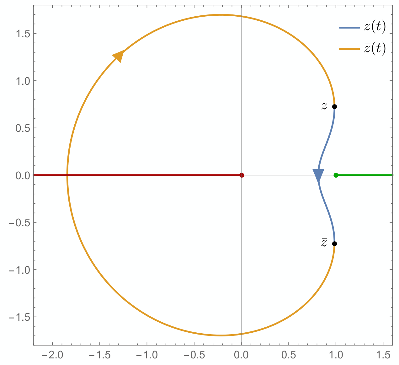
Let us conclude by discussing how the analytic continuation changes if other Wilson lines are incoming.
- •
If the Wilson lines 1 and 4 (or 2 and 3) are incoming, then only acquires a phase:
(5.11) Repeating the previous analysis, one finds that avoids all branch cuts, while crosses the branch cut starting at in the clockwise direction. The imaginary part can be determined in a way similar to the previous case, by using the shuffle algebra to make all discontinuities at explicit:
(5.12) - •
If the Wilson lines 1 and 3 (or 2 and 4) are incoming, then both and acquire a phase:
(5.13) This time both and cross branch cuts starting at and , respectively, going counterclockwise. This is equivalent to the contour drawn by and together encircling the branch point at infinity in the clockwise direction, and we can extract the imaginary parts as in the previous cases.
We have thus seen that analytic continuation to the physical region of -to- scattering takes the function away from the region where it is single-valued, generating imaginary parts. Thus after analytic continuation the function will be expressed in terms of ordinary harmonic polylogarithms. We have also seen that for each pair of incoming particles, there is a distinct branch point – one of the three – which is encircled by the combined trajectory of and .
B. The momentum conserving limit.
Having performed the analytic continuation, our ansatz is now valid in the region where two specific partons are incoming. Below we only discuss the case where the partons 1 and 2 are incoming, and all other cases are similar. The kinematics does not yet correspond to a massless 2-to-2 scattering, because this requires momentum conservation among the partonic momenta, in addition to the constraint , with and . Since we will be interested in the Regge limit , we can assume without loss of generality that we work in a region where is greater than . Imposing these constraints, we see that the cross ratios become
| (5.14) |
It is easy to check that in the momentum conserving limit eq. (4.6) implies:
| (5.15) |
Having started from a complex conjugate pair, , the momentum conserving limit corresponds to the situation where and approach the real axis. Care is needed, however, because and approach the real axis from opposite sides. Indeed, if we assume that in the Euclidean region and were in the upper and lower half planes respectively, then after analytic continuation and have negative and positive imaginary parts, respectively. Hence, in the momentum conserving limit approaches the real axis from below, while approaches it from above. Equation (5.15) then implies that some harmonic polylogarithms may develop opposite imaginary parts in the limit, e.g.,
| (5.16) | ||||
| (5.17) |
Let us conclude by commenting on the class of functions that appear in the momentum conserving limit. Since , we can write entirely in terms of ordinary HPLs in the single variable , in agreement with all known results for on-shell four-point amplitudes in QCD and SYM [120, 121, 122, 123, 124, 125, 104, 126, 127, 128, 129, 109].
C. Constraints from the Regge limit.
Having at our disposal the ansatz in the physical region of a 2-to-2 scattering, we can proceed and consider its Regge limit. There are three different choices for the incoming particles, and for each choice we can consider two different Regge limits, corresponding to forward and backward scattering. In the following we discuss one of these limits in detail, and we only comment on the other limits at the very end.
Let us consider the Regge limit of the scattering where the partons 1 and 2 are incoming and . We know that our ansatz can be written in terms of HPLs in , and we can expand each HPL in a power series in . Dropping power-suppressed terms, we find that the functions in eq. (4.13) reduce to
| (5.18) |
and
| (5.19) | ||||
where we have adopted the notation . These expressions can be compared to the results of ref. [73, 35], as mentioned above. This requires the coefficients of , with in the real part of the amplitude and in the imaginary part, to vanish in eqs. (5.18) and (5.19). We then find six independent conditions on the undetermined coefficients in our ansatz for .
We have carried out the same analysis in the remaining five Regge limits, and the expansion of our ansatz in two of these limits – where partons 1 and 3 are incoming and , and where partons 1 and 4 are incoming and – are presented in Appendix A. Each Regge limit gives rise to six constraints, but those coming from limits involving the same pairs of incoming (or outgoing) partons are identical. Any pair of Regge limits involving different incoming (or outgoing) partons gives rise to eight independent constraints between them, after which considering additional Regge limits doesn’t give rise to further constraints. Putting together the constraints from the above Regge limit and one of the limits considered in Appendix A, we can thus fix 8 out of the 13 free parameters in our ansatz in eq. (4.18):
| (5.20) | ||||
Having discussed the Regge limit in detail, we now turn to the kinematic limit in which two Wilson lines become collinear.
6 The collinear limit
6.1 Collinear limits
As has already been considered in refs. [29, 32], further kinematic constraints on the soft anomalous dimension arise from collinear limits. We briefly review this argument here. Let us now work in the kinematic region where all coloured particles carrying momenta are outgoing, and consider the limit in which two of these partons, and , become collinear. In this limit , resulting in kinematic divergences inversely proportional to . It is well known that for final-state collinear partons88 8 In the case of a space-like splitting, factorisation is violated [130, 131]. these divergences factorise [132, 133, 134, 135], such that one may write
| (6.1) |
Without loss of generality, we have taken particles 1 and 2 collinear, where , denotes the set of remaining momenta. The right-hand side contains the -particle amplitude in which the momenta and are replaced by the sum , multiplied by a universal splitting function , which collects all singular contributions to the amplitude due to particles 1 and 2 becoming collinear. Care must be taken to interpret the colour structure of eq. (6.1). The amplitudes and live in -parton and -parton colour space respectively. However, one may write a colour generator on the line of momentum as
| (6.2) |
which promotes the amplitude to live in -parton colour space after all. Crucially, the splitting amplitudes must only depend on the quantum numbers of particles 1 and 2. It is this property that we wish to exploit, following refs. [29, 32], in order to constrain the soft anomalous dimension. Let us briefly recall how the constraint arises, before analysing its implications regarding our ansatz.
One starts with the observation that infrared factorization, according to eq. (2.5), holds separately for the and -parton99 9 Note that in eq. (6.1) is evaluated at , and hence it obeys the usual soft-collinear factorisation formula for massless partons scattering in eq. (2.1). amplitudes in eq. (6.1):
| (6.3a) | ||||
| (6.3b) | ||||
Kinematic divergences in the collinear limit appear in eq. (6.3a) in both and the hard function . By analogy with eq. (6.1), the hard function may be factorised in the collinear limit according to
| (6.4) |
where is an appropriate splitting function collecting all terms which are singular as , such that the -particle hard function may be evaluated with . Of course, all quantities in eq. (6.4) are infrared finite.
Equations (6.3) together with eqs. (6.1) and (6.4) implies the condition
| (6.5) | ||||
where all quantities must be evaluated in the limit . This equation implies a highly non-trivial cancellation between both colour and kinematic dependence on the right-hand side, such that the left-hand side depends only on the quantum numbers of the two particles becoming collinear.
Given that the amplitude splitting function does not depend on the infrared factorisation scale , one may differentiate eq. (6.5) and use eq. (2.6) to obtain the condition
| (6.6) |
where we have defined
| (6.7) |
Given that the quantity on the left-hand side of this equation depends manifestly on the quantum numbers of partons 1 and 2 only, this must also be true for the right-hand side. Upon making the decomposition of eq. (2.11) (valid up to three-loop order), one may further decompose
| (6.8) | ||||
We want to take the kinematic limit in which partons 1 and 2 become collinear. To this end, we may parametrise each momentum according to:
| (6.9) |
where is a small momentum to allow , while . The first term in eq. (6.8) is then found to be [32]
| (6.10) | ||||
in terms of the quantities appearing in eq. (2.8). Note that here as we assumed that and both belong to the final state. Equation (6.10) by itself depends only on the quantum numbers of the two particles becoming collinear, which finally leads to an important constraint on the , namely that the difference
| (6.11) |
can only depend on the quantum numbers of the two particles that are becoming collinear. Note that the right-hand side of eq. (6.11) is evaluated in the limit where and have become collinear. As suggested by our notation, this quantity has no kinematic dependence. To see this, first note that universality of the splitting function implies that the result should be independent of the number of Wilson lines . When , colour conservation implies that there is only one independent colour structure (a single quadratic Casimir), such that the dipole formula furnishes the complete splitting function, and the correction term vanishes: . This in turn implies
| (6.12) |
but since there are no conformally invariant cross ratios that one can form from three particle momenta, the right-hand side evaluates to a constant. Universality of the splitting amplitude then implies that the same is true for all .
6.2 Constraints from two-particle collinear limits
Equation (6.11) dictates that when two partons become collinear, the difference can only depend on the colour and kinematic degrees of freedom of the two partons becoming collinear. In fact, we saw that this difference must be a constant, independent of the number of Wilson lines (provided one takes , so that ). These properties can be imposed as further constraints on our ansatz for . To do so, we specialize to three- and four-parton scattering, and set . We do not impose momentum conservation (i.e. we consider the situation in which any number of colour singlet particles may carry additional momentum). This will allow us to consider pairs of particles becoming collinear, without simultaneously restricting the momenta of other coloured particles. We also choose to focus on the collinear limit in which . It will prove convenient to define the basis of colour generators as follows [102]:
| (6.13) | ||||
Note that in contrast with the generators corresponding to different lines the generators defined in eq. (6.13) are not mutually commuting. The nonzero commutators amongst them are summarised by eq. (B.4).
Let us first consider the case, for which colour conservation assumes the form
| (6.14) |
As we saw in eq. (6.12), the difference in eq. (6.11) reduces to the single term when . In addition, for this number of partons the second and third lines in eq. (2.15) are not present, as they consist of sums over four particle combinations only. We thus have
| (6.15) |
One can put this in a form where colour conservation is made explicit using eq. (6.14), after commuting all factors of to the right. Making liberal use of the colour identities listed in appendix B, one can put this in the form
| (6.16) |
where is the part of our ansatz defined in eq. (4.19). As the right-hand side of this equation is already a constant and depends only on the colour degrees of freedom of particles 1 and 2, it does not directly constrain our ansatz. However, we can now require that the right hand side of eq. (6.11) equals this expression when evaluated for any number of partons .
With this in mind, we now turn to the case. Using the definitions in eq. (6.13) again, colour conservation can be written as
| (6.17) |
Moreover, the second term in eq. (6.11) becomes (cf. eq. (6.15))
| (6.18) | ||||
After expressing all colour generators in terms of the basis of eq. (6.13), one may commute all factors of to the right, and then implement colour conservation according to eq. (6.17). Using the identities in appendix B one then obtains
| (6.19) |
To put the first term in eq. (6.11) into a form that manifests colour conservation, we first use the Jacobi identity to rewrite the expression in eq. (2.15) for general and as
| (6.20) | ||||
Again employing colour conservation after moving to the right and simplifying, the sum over colour structures in the first term of eq. (6.20) can be rewritten as
| (6.21) | ||||
By a similar procedure, the remaining colour structures in eq. (6.20) evaluate to
| (6.22a) | ||||
| (6.22b) | ||||
Substituting these expressions back into eq. (6.20) and subtracting eq. (6.19), one obtains
| (6.23) |
As discussed above, consistency of collinear factorisation means that the right-hand side of eq. (6.23) must only depend on the degrees of freedom of particles 1 and 2. This in turn means that dependence on in the collinear limit is forbidden, which immediately implies the constraints
| (6.24) |
Implementing these in eq. (6.23) we find that the latter indeed becomes equal to eq. (6.16). Thus, the quantity is indeed found to be universal, in that it is independent of whether one considers three or four-parton scattering. The constraints of eq. (6.24) can be recast in the form
| (6.25) |
where we used eq. (4.11) to write the relevant combinations of in terms of and subsequently related them to the , , defined in eq. (4.13), getting:
| (6.26) |
where and where we used eq. (4.15) to write in terms of . The interpretation of the two conditions in eq. (6.25) becomes clear upon comparing eq. (6.20) to eq. (4.17): the first condition corresponds to the component in which is antisymmetric in both colour and kinematics variables of lines 1 and 2, and so must clearly vanish when , while the latter corresponds to the symmetric component, which instead approaches a non-zero constant in this collinear limit.
Considering the leading behaviour of the kinematic variables in the collinear limit , one finds
| (6.27) | ||||
where all phases cancel, having assumed that all particles are outgoing (as far as the cross ratios are concerned, this is equivalent to working in the Euclidean region). These conditions together imply
| (6.28) |
in which limit reduces to a polynomial in with coefficients drawn from the space of multiple zeta values. It is easy to see that the condition on in eq. (6.25) is always satisfied, and thus does not provide any constraint on the coefficients , because
| (6.29) |
Conversely, plugging the ansatz of eq. (4.18) into eq. (6.25), using eq. (6.26) and taking the leading collinear behaviour as , we find
| (6.30) | ||||
which is not generically a constant, as eq. (6.25) tells us it must be. Requiring all the non-constant terms in to vanish gives us the constraints
| (6.31) |
Moreover, we can use the condition in eq. (6.25) to place constraints on the parameters and that enter our ansatz for in eq. (4.19). That is, imposing the constraints in eqs. (5.20) and (6.31) on and equating it to implies
| (6.32) |
Here we have considered particles 1 and 2 becoming collinear such that , and leading to the conditions:
| (6.33) |
corresponding to the antisymmetric and symmetric parts in eq. (4.17) under permutation of {1,2}. We may also consider the limits in which the pair of particles {1,3} or {1,4} become collinear, implying and respectively.1010 10 The remaining collinear limits in which particles {2,3}, {2,4} or {3,4} become collinear correspond to the same limits of , and thus provide no complementary information. The above arguments can be repeated to show that in the limit , one obtains the conditions
| (6.34) |
and similarly if :
| (6.35) |
The conditions of eqs. (6.34) and (6.35) can be seen to coincide with eq. (6.33) upon using the transformations of eq. (4.9), or equivalently they can be simply deduced from eq. (6.33) using the relations in eq. (4.15). Thus, the additional collinear limits provide no complementary information. In summary, the collinear limit provides the following constraints on the parameters :
| (6.36) |
7 Discussion
In the previous two sections, we have derived separate constraints on the parameters entering the ansätze of eqs. (4.18) and (4.19), from both the Regge and collinear limits, as summarised in eqs. (5.20) and (6.36) respectively. We can now combine them into a single set. In doing so, we see that the first two conditions in eq. (6.36) are already contained in eq. (5.20), but that the remaining ones are complementary. Upon implementing the full set of constraints, the ansätze of eqs. (4.18) and (4.19) reduce to
| (7.1) |
We see that both and have been uniquely determined by our bootstrap procedure, up to an overall rational number . Since depends linearly on and , the form of the three-loop correction to the dipole formula is fixed completely by symmetries and physical constraints. Comparing the expressions in eq. (7.1) with the result of ref. [58] (quoted here in eqs. (2.19) and (2.16)), we see that the latter can be reproduced by setting . Our analysis is a highly non-trivial cross-check of the results of ref. [58], as well as the consistency of the bootstrap procedure. This is the first time that a bootstrap procedure has been successfully applied to a quantity in non-planar perturbative gauge theory.
It is interesting to observe the complementary nature of the Regge and collinear limits used here. While the number of constraints that arise from the Regge limit is larger – notably because it provides information on both the real and imaginary parts of the amplitude at each logarithmic order – it is the collinear limit that relates the function and the constant . This non-trivial interplay between the four- and three-line structures is a manifestation of colour conservation, or the gauge invariance of the theory. In principle such a relation could arise from the Regge limit as well, but it requires extending computations along the lines of refs. [35, 73] to higher logarithmic accuracy.
Given the homogeneous nature of all our collinear and Regge constraints, we cannot use them to fix the overall normalisation of . Had it not been computed, one could consider fixing this constant by various other means. For example, it could be determined by numerical integration at suitably high precision at a single kinematic point. Other options include analytically computing the simpler quantity , which is just a constant, or extracting the overall normalization factor from the three-loop four-point amplitude in SYM [109]. Alternatively, could be fixed by the knowledge of a non-homogeneous constraint, such as the computation of the term in the Regge limit of 2-to-2 scattering, which is known to receive non-vanishing contributions from [73].
The fact that the form of is fixed by symmetries and dynamic constraints begs the question as to whether the same is true at higher loop orders. Before such a program can be carried out, however, one must take into account the fact that the structure of the soft anomalous dimension becomes more complicated starting at four loops. This is due to the breakdown of Casimir scaling in the cusp anomalous dimension, which was recently demonstrated in ref. [78] and requires modifying the dipole formula starting at four loops. The contribution to the soft anomalous dimension depending only on conformally-invariant cross ratios will still be amenable to the methods employed here. In particular, we have argued that this contribution can be expressed in terms of single-valued polylogarithms to all loop orders. However, starting at four loops also becomes sensitive to the matter content of the theory, meaning that the assumptions of uniform transcendental weight and purity will not generically apply. Additionally, as mentioned in section 3, single-valued polylogarithms depending on more than one complex variable are expected to appear, since more than four Wilson lines can become correlated in higher-loop diagrams. Even so, the types of constraints considered in this paper also generalize to higher loops. In fact, the requirement that the amplitude factorizes in two-particle collinear limits can be directly applied at any loop order [132, 133, 134, 135]. Further computations are required to extend the types of Regge constraints we have used in the present paper to higher loops, but there exists a well-defined framework to study the Regge limit of QCD amplitudes at arbitrary order [35, 119, 73], making it possible for the relevant computations to be carried out. In particular, it is possible to explore constraints coming from multi-Regge limits [34, 33] in addition to single-Regge limits. Lastly, one can consider multi-particle collinear limits, in which higher-particle Mandelstam invariants go on shell. The multi-particle limits of the three-loop soft anomalous dimension have already been computed, and do not give rise to any constraints on beyond those implied by two-particle collinear limits [136]. However, they could provide additional information at higher loop orders.
Finally, it would be interesting to see if a similar bootstrap procedure could be applied to other physical quantities of interest. The extension of our work to the massive three-loop soft anomalous dimension is currently hampered by our lack of understanding of the corresponding space of functions, i.e., iterated integrals on hyperbolic 3-space, as discussed in section 3. Conversely, the single-emission soft current is known to be expressible in terms of SVHPLs through two loops from the calculations of ref. [137, 138, 139, 140], suggesting that this quantity may also be amenable to bootstrap techniques. It can also be hoped that it will eventually prove possible to bootstrap QCD amplitudes themselves; however, a much better understanding of the functions appearing in these amplitudes is required before any such approach can be attempted.
Acknowledgments
We are grateful for Lance Dixon, Sebastian Jaskiewicz, Jeffrey Pennington and Leonardo Vernazza for stimulating discussions. We would like to thank the ESI institute in Vienna and the organisers of the program “Challenges and Concepts for Field Theory and Applications in the Era of LHC Run-2,” Nordita in Stockholm and the organisers of “Aspects of Amplitudes” over the summer of 2016 and the CERN TH Institute “LHC and the Standard Model: Physics and Tools”. CD, AM & CDW acknowledge the hospitality of the Higgs Centre of the University of Edinburgh at various stages of this work. This work is supported by the European Research Council (ERC) under the Horizon 2020 Research and Innovation Programme through the grant 637019 “MathAm”, by the National Science Foundation under Grant No. NSF PHY11-25915, and by the STFC Consolidated Grants “Particle Physics at the Higgs Centre” and “String Theory, Gauge Theory and Duality”.
Appendix A Alternative Regge limits
In this appendix, we give the forms of the ansatz of eq. (4.18) in some alternative Regge limits to that considered in section 5, using the analytic continuations of eqs. (5.11) and (5.13). We first consider particles 1 and 3 to be incoming. Then, in the Regge limit , the real and imaginary parts of the functions of eq. (4.13) become (with )
| (A.1) |
and
| (A.2) | ||||
respectively.
Next, we consider particles 1 and 4 to be incoming, and the Regge limit . In this case, one finds (now with )
| (A.3) |
and
| (A.4) | ||||
Appendix B Useful colour identities
Here, we collect a number of colour algebra identities that are useful when applying the collinear constraint in section 6.2. Contraction of a pair of structure constants gives
| (B.1) |
Then the Jacobi identity of eq. (4.12) implies
| (B.2) |
We also make use of a number of useful identities resulting from antisymmetry of the structure constants under interchange of any two indices:
| (B.3) | ||||
where is an arbitrary antisymmetric matrix of dimension , and the last identity holds for any invertible map .
Finally, the non-zero commutators among the colour operators defined in eq. (6.13) are
| (B.4) |
These are useful for applying colour conservation in this basis.
References
- [1] A. M. Polyakov, “Gauge Fields as Rings of Glue,” Nucl. Phys. B164 (1980) 171–188.
- [2] I. Y. Arefeva, “Quantum contour field equations,” Phys. Lett. B93 (1980) 347–353.
- [3] V. S. Dotsenko and S. N. Vergeles, “Renormalizability of Phase Factors in the Nonabelian Gauge Theory,” Nucl. Phys. B169 (1980) 527.
- [4] R. A. Brandt, F. Neri, and M.-a. Sato, “Renormalization of Loop Functions for All Loops,” Phys. Rev. D24 (1981) 879.
- [5] G. P. Korchemsky and A. V. Radyushkin, “Loop space formalism and renormalization group for the infrared asymptotics of QCD,” Phys. Lett. B171 (1986) 459–467.
- [6] G. Korchemsky and A. Radyushkin, “Infrared asymptotics of perturbative QCD: Renormalization properties of the wilson loops in higher orders of perturbation theory,” Sov. J. Nucl. Phys. 44 (1986) 877.
- [7] G. Korchemsky and A. Radyushkin, “Renormalization of the Wilson Loops Beyond the Leading Order,” Nucl. Phys. B283 (1987) 342–364.
- [8] A. H. Mueller, “On the asymptotic behavior of the Sudakov form-factor,” Phys. Rev. D20 (1979) 2037.
- [9] J. C. Collins, “Algorithm to compute corrections to the Sudakov form-factor,” Phys. Rev. D22 (1980) 1478.
- [10] A. Sen, “Asymptotic Behavior of the Sudakov Form-Factor in QCD,” Phys. Rev. D24 (1981) 3281.
- [11] A. Sen, “Asymptotic Behavior of the Wide Angle On-Shell Quark Scattering Amplitudes in Nonabelian Gauge Theories,” Phys. Rev. D28 (1983) 860.
- [12] J. G. M. Gatheral, “Exponentiation of eikonal cross-sections in nonabelian gauge theories,” Phys. Lett. B133 (1983) 90.
- [13] J. Frenkel and J. C. Taylor, “Nonabelian eikonal exponentiation,” Nucl. Phys. B246 (1984) 231.
- [14] G. F. Sterman, “Infrared divergences in perturbative QCD. (talk),” AIP Conf. Proc. 22–40.
- [15] L. Magnea and G. F. Sterman, “Analytic continuation of the Sudakov form-factor in QCD,” Phys. Rev. D42 (1990) 4222–4227.
- [16] G. P. Korchemsky, “On Near forward high-energy scattering in QCD,” Phys. Lett. B325 (1994) 459–466, hep-ph/9311294.
- [17] I. Korchemskaya and G. Korchemsky, “Evolution equation for gluon Regge trajectory,” Phys. Lett. B387 (1996) 346–354, hep-ph/9607229.
- [18] I. Korchemskaya and G. Korchemsky, “High-energy scattering in QCD and cross singularities of Wilson loops,” Nucl. Phys. B437 (1995) 127–162, hep-ph/9409446.
- [19] S. Catani and M. H. Seymour, “A general algorithm for calculating jet cross sections in NLO QCD,” Nucl. Phys. B485 (1997) 291–419, hep-ph/9605323.
- [20] S. Catani, “The Singular behavior of QCD amplitudes at two loop order,” Phys. Lett. B427 (1998) 161–171, hep-ph/9802439.
- [21] G. F. Sterman and M. E. Tejeda-Yeomans, “Multi-loop amplitudes and resummation,” Phys. Lett. B552 (2003) 48–56, hep-ph/0210130.
- [22] L. J. Dixon, L. Magnea, and G. Sterman, “Universal structure of subleading infrared poles in gauge theory amplitudes,” JHEP 08 (2008) 022, 0805.3515.
- [23] N. Kidonakis, G. Oderda, and G. F. Sterman, “Evolution of color exchange in QCD hard scattering,” Nucl. Phys. B531 (1998) 365–402, hep-ph/9803241.
- [24] R. Bonciani, S. Catani, M. L. Mangano, and P. Nason, “Sudakov resummation of multiparton QCD cross-sections,” Phys. Lett. B575 (2003) 268–278, hep-ph/0307035.
- [25] Yu. L. Dokshitzer and G. Marchesini, “Soft gluons at large angles in hadron collisions,” JHEP 01 (2006) 007, hep-ph/0509078.
- [26] S. M. Aybat, L. J. Dixon, and G. F. Sterman, “The two-loop soft anomalous dimension matrix and resummation at next-to-next-to leading pole,” Phys. Rev. D74 (2006) 074004, hep-ph/0607309.
- [27] E. Gardi and L. Magnea, “Factorization constraints for soft anomalous dimensions in QCD scattering amplitudes,” JHEP 0903 (2009) 079, 0901.1091.
- [28] T. Becher and M. Neubert, “Infrared singularities of scattering amplitudes in perturbative QCD,” Phys. Rev. Lett. 102 (2009) 162001, 0901.0722.
- [29] T. Becher and M. Neubert, “On the Structure of Infrared Singularities of Gauge-Theory Amplitudes,” JHEP 06 (2009) 081, 0903.1126.
- [30] E. Gardi and L. Magnea, “Infrared singularities in QCD amplitudes,” Nuovo Cim. 032C (2009) 137–157, 0908.3273.
- [31] L. J. Dixon, “Matter Dependence of the Three-Loop Soft Anomalous Dimension Matrix,” Phys. Rev. D79 (2009) 091501, 0901.3414.
- [32] L. J. Dixon, E. Gardi, and L. Magnea, “On soft singularities at three loops and beyond,” JHEP 02 (2010) 081, 0910.3653.
- [33] V. Del Duca, C. Duhr, E. Gardi, L. Magnea, and C. D. White, “An infrared approach to Reggeization,” Phys. Rev. D85 (2012) 071104, 1108.5947.
- [34] V. Del Duca, C. Duhr, E. Gardi, L. Magnea, and C. D. White, “The Infrared structure of gauge theory amplitudes in the high-energy limit,” JHEP 1112 (2011) 021, 1109.3581.
- [35] S. Caron-Huot, “When does the gluon reggeize?,” JHEP 05 (2015) 093, 1309.6521.
- [36] V. Ahrens, M. Neubert, and L. Vernazza, “Structure of Infrared Singularities of Gauge-Theory Amplitudes at Three and Four Loops,” JHEP 1209 (2012) 138, 1208.4847.
- [37] S. G. Naculich, H. Nastase, and H. J. Schnitzer, “All-loop infrared-divergent behavior of most-subleading-color gauge-theory amplitudes,” JHEP 1304 (2013) 114, 1301.2234.
- [38] O. Erdoğan and G. Sterman, “Ultraviolet divergences and factorization for coordinate-space amplitudes,” Phys. Rev. D91 (2015), no. 6, 065033, 1411.4588.
- [39] T. Gehrmann, E. W. N. Glover, T. Huber, N. Ikizlerli, and C. Studerus, “Calculation of the quark and gluon form factors to three loops in QCD,” JHEP 06 (2010) 094, 1004.3653.
- [40] N. Kidonakis, “Two-loop soft anomalous dimensions and NNLL resummation for heavy quark production,” Phys. Rev. Lett. 102 (2009) 232003, 0903.2561.
- [41] A. Mitov, G. Sterman, and I. Sung, “The Massive Soft Anomalous Dimension Matrix at Two Loops,” Phys. Rev. D79 (2009) 094015, 0903.3241.
- [42] T. Becher and M. Neubert, “Infrared singularities of QCD amplitudes with massive partons,” Phys. Rev. D79 (2009) 125004, 0904.1021.
- [43] M. Beneke, P. Falgari, and C. Schwinn, “Soft radiation in heavy-particle pair production: all- order colour structure and two-loop anomalous dimension,” Nucl. Phys. B828 (2010) 69–101, 0907.1443.
- [44] M. Czakon, A. Mitov, and G. F. Sterman, “Threshold Resummation for Top-Pair Hadroproduction to Next-to-Next-to-Leading Log,” Phys. Rev. D80 (2009) 074017, 0907.1790.
- [45] A. Ferroglia, M. Neubert, B. D. Pecjak, and L. L. Yang, “Two-loop divergences of massive scattering amplitudes in non-abelian gauge theories,” JHEP 11 (2009) 062, 0908.3676.
- [46] J.-y. Chiu, A. Fuhrer, R. Kelley, and A. V. Manohar, “Factorization Structure of Gauge Theory Amplitudes and Application to Hard Scattering Processes at the LHC,” Phys. Rev. D80 (2009) 094013, 0909.0012.
- [47] A. Mitov, G. F. Sterman, and I. Sung, “Computation of the Soft Anomalous Dimension Matrix in Coordinate Space,” Phys. Rev. D82 (2010) 034020, 1005.4646.
- [48] E. Gardi, “From Webs to Polylogarithms,” JHEP 1404 (2014) 044, 1310.5268.
- [49] G. Falcioni, E. Gardi, M. Harley, L. Magnea, and C. D. White, “Multiple Gluon Exchange Webs,” JHEP 10 (2014) 10, 1407.3477.
- [50] J. M. Henn, A. V. Smirnov, and V. A. Smirnov, “Analytic results for planar three-loop four-point integrals from a Knizhnik-Zamolodchikov equation,” JHEP 07 (2013) 128, 1306.2799.
- [51] M. Dukes, E. Gardi, H. McAslan, D. J. Scott, and C. D. White, “Webs and Posets,” 1310.3127.
- [52] M. Dukes, E. Gardi, E. Steingrimsson, and C. D. White, “Web worlds, web-colouring matrices, and web-mixing matrices,” J. Comb. Theory Ser. A 120 (2013) 1012–1037, 1301.6576.
- [53] E. Gardi, E. Laenen, G. Stavenga, and C. D. White, “Webs in multiparton scattering using the replica trick,” JHEP 1011 (2010) 155, 1008.0098.
- [54] E. Gardi and C. D. White, “General properties of multiparton webs: Proofs from combinatorics,” JHEP 1103 (2011) 079, 1102.0756.
- [55] E. Gardi, J. M. Smillie, and C. D. White, “On the renormalization of multiparton webs,” JHEP 1109 (2011) 114, 1108.1357.
- [56] E. Gardi, J. M. Smillie, and C. D. White, “The Non-Abelian Exponentiation theorem for multiple Wilson lines,” JHEP 06 (2013) 088, 1304.7040.
- [57] E. Laenen, G. Stavenga, and C. D. White, “Path integral approach to eikonal and next-to-eikonal exponentiation,” JHEP 03 (2009) 054, 0811.2067.
- [58] Ø. Almelid, C. Duhr, and E. Gardi, “Three-loop corrections to the soft anomalous dimension in multileg scattering,” Phys. Rev. Lett. 117 (2016), no. 17, 172002, 1507.00047.
- [59] F. C. S. Brown, “Single-valued multiple polylogarithms in one variable,” C. R. Acad. Sci. Paris Ser. I (2004) 338.
- [60] E. Remiddi and J. Vermaseren, “Harmonic polylogarithms,” Int.J.Mod.Phys. A15 (2000) 725–754, hep-ph/9905237.
- [61] L. J. Dixon, C. Duhr, and J. Pennington, “Single-valued harmonic polylogarithms and the multi-Regge limit,” JHEP 10 (2012) 074, 1207.0186.
- [62] L. J. Dixon, J. M. Drummond, and J. M. Henn, “Bootstrapping the three-loop hexagon,” JHEP 11 (2011) 023, 1108.4461.
- [63] L. J. Dixon, J. M. Drummond, and J. M. Henn, “Analytic result for the two-loop six-point NMHV amplitude in N=4 super Yang-Mills theory,” JHEP 01 (2012) 024, 1111.1704.
- [64] L. J. Dixon, J. M. Drummond, M. von Hippel, and J. Pennington, “Hexagon functions and the three-loop remainder function,” JHEP 12 (2013) 049, 1308.2276.
- [65] L. J. Dixon, J. M. Drummond, C. Duhr, and J. Pennington, “The four-loop remainder function and multi-Regge behavior at NNLLA in planar N = 4 super-Yang-Mills theory,” JHEP 06 (2014) 116, 1402.3300.
- [66] L. J. Dixon and M. von Hippel, “Bootstrapping an NMHV amplitude through three loops,” JHEP 10 (2014) 065, 1408.1505.
- [67] L. J. Dixon, M. von Hippel, and A. J. McLeod, “The four-loop six-gluon NMHV ratio function,” JHEP 01 (2016) 053, 1509.08127.
- [68] S. Caron-Huot, L. J. Dixon, A. McLeod, and M. von Hippel, “Bootstrapping a Five-Loop Amplitude Using Steinmann Relations,” Phys. Rev. Lett. 117 (2016), no. 24, 241601, 1609.00669.
- [69] J. M. Drummond, G. Papathanasiou, and M. Spradlin, “A Symbol of Uniqueness: The Cluster Bootstrap for the 3-Loop MHV Heptagon,” JHEP 03 (2015) 072, 1412.3763.
- [70] L. J. Dixon, J. Drummond, T. Harrington, A. J. McLeod, G. Papathanasiou, and M. Spradlin, “Heptagons from the Steinmann Cluster Bootstrap,” JHEP 02 (2017) 137, 1612.08976.
- [71] V. Del Duca, G. Falcioni, L. Magnea, and L. Vernazza, “High-energy QCD amplitudes at two loops and beyond,” Phys. Lett. B732 (2014) 233–240, 1311.0304.
- [72] V. Del Duca, G. Falcioni, L. Magnea, and L. Vernazza, “Analyzing high-energy factorization beyond next-to-leading logarithmic accuracy,” JHEP 02 (2015) 029, 1409.8330.
- [73] S. Caron-Huot, E. Gardi, and L. Vernazza, “Two-parton scattering in the high-energy limit,” JHEP 06 (2017) 016, 1701.05241.
- [74] E. Gardi, Ø. Almelid, and C. Duhr, “Long-distance singularities in multi-leg scattering amplitudes,” PoS LL2016 (2016) 058, 1606.05697.
- [75] S. Moch, J. Vermaseren, and A. Vogt, “The Three loop splitting functions in QCD: The Nonsinglet case,” Nucl. Phys. B688 (2004) 101–134, hep-ph/0403192.
- [76] A. Grozin, J. M. Henn, G. P. Korchemsky, and P. Marquard, “Three Loop Cusp Anomalous Dimension in QCD,” Phys. Rev. Lett. 114 (2015), no. 6, 062006, 1409.0023.
- [77] S. Moch, J. A. M. Vermaseren, and A. Vogt, “Three-loop results for quark and gluon form-factors,” Phys. Lett. B625 (2005) 245–252, hep-ph/0508055.
- [78] R. H. Boels, T. Huber, and G. Yang, “The four-loop non-planar cusp anomalous dimension in N = 4 SYM,” 1705.03444.
- [79] F. C. S. Brown, “Multiple zeta values and periods of moduli spaces M 0 ,n ( R ),” Annales Sci. Ecole Norm. Sup. 42 (2009) 371, math/0606419.
- [80] K. T. Chen, “Iterated path integrals,” Bull. Amer. Math. Soc. 83 (1977) 831.
- [81] A. B. Goncharov, “Multiple polylogarithms, cyclotomy and modular complexes,” Math. Res. Lett. 5 (1998) 497–516, 1105.2076.
- [82] A. B. Goncharov, “Galois symmetries of fundamental groupoids and noncommutative geometry,” Duke Math. J. 128 (2005), no. 2, 209.
- [83] A. Goncharov, “A simple construction of Grassmannian polylogarithms,” 0908.2238.
- [84] C. Duhr, H. Gangl, and J. R. Rhodes, “From polygons and symbols to polylogarithmic functions,” JHEP 1210 (2012) 075, 1110.0458.
- [85] F. Brown, “On the decomposition of motivic multiple zeta values,” 1102.1310.
- [86] C. Duhr, “Hopf algebras, coproducts and symbols: an application to Higgs boson amplitudes,” JHEP 1208 (2012) 043, 1203.0454.
- [87] F. C. S. Brown, “Notes on motivic periods,” 1512.06410.
- [88] D. Gaiotto, J. Maldacena, A. Sever, and P. Vieira, “Pulling the straps of polygons,” JHEP 12 (2011) 011, 1102.0062.
- [89] S. Abreu, R. Britto, and H. Grönqvist, “Cuts and coproducts of massive triangle diagrams,” JHEP 07 (2015) 111, 1504.00206.
- [90] F. Chavez and C. Duhr, “Three-mass triangle integrals and single-valued polylogarithms,” JHEP 11 (2012) 114, 1209.2722.
- [91] O. Schnetz, “Graphical functions and single-valued multiple polylogarithms,” Commun. Num. Theor. Phys. 08 (2014) 589–675, 1302.6445.
- [92] J. Drummond, C. Duhr, B. Eden, P. Heslop, J. Pennington, and V. A. Smirnov, “Leading singularities and off-shell conformal integrals,” JHEP 08 (2013) 133, 1303.6909.
- [93] V. Del Duca, L. J. Dixon, C. Duhr, and J. Pennington, “The BFKL equation, Mueller-Navelet jets and single-valued harmonic polylogarithms,” JHEP 02 (2014) 086, 1309.6647.
- [94] V. Del Duca, S. Druc, J. Drummond, C. Duhr, F. Dulat, R. Marzucca, G. Papathanasiou, and B. Verbeek, “Multi-Regge kinematics and the moduli space of Riemann spheres with marked points,” JHEP 08 (2016) 152, 1606.08807.
- [95] J. Broedel, M. Sprenger, and A. Torres Orjuela, “Towards single-valued polylogarithms in two variables for the seven-point remainder function in multi-Regge-kinematics,” Nucl. Phys. B915 (2017) 394–413, 1606.08411.
- [96] O. Schnetz, “Numbers and Functions in Quantum Field Theory,” 1606.08598.
- [97] V. Del Duca, C. Duhr, R. Marzucca, and B. Verbeek, “The analytic structure and the transcendental weight of the BFKL ladder at NLL accuracy,” 1705.10163.
- [98]
F. C. S. Brown, “Single-valued hyperlogarithms and unipotent differential
equations,”
http://www.ihes.fr/~brown/RHpaper5.pdf. - [99] F. Brown, “Single-valued Motivic Periods and Multiple Zeta Values,” SIGMA 2 (2014) e25, 1309.5309.
- [100] Y.-T. Chien, M. D. Schwartz, D. Simmons-Duffin, and I. W. Stewart, “Jet Physics from Static Charges in AdS,” Phys. Rev. D85 (2012) 045010, 1109.6010.
- [101] C. Cheung, A. de la Fuente, and R. Sundrum, “4D scattering amplitudes and asymptotic symmetries from 2D CFT,” JHEP 01 (2017) 112, 1609.00732.
- [102] Ø. Almelid, The Three-Loop Soft Anomalous Dimension of Massless Multileg Scattering. PhD thesis, University of Edinburgh, 2016.
- [103] Ø. Almelid, C. Duhr, and E. Gardi. In preparation.
- [104] Z. Bern, L. J. Dixon, and V. A. Smirnov, “Iteration of planar amplitudes in maximally supersymmetric Yang-Mills theory at three loops and beyond,” Phys. Rev. D72 (2005) 085001, hep-th/0505205.
- [105] V. Del Duca, C. Duhr, and V. A. Smirnov, “An Analytic Result for the Two-Loop Hexagon Wilson Loop in N = 4 SYM,” JHEP 03 (2010) 099, 0911.5332.
- [106] V. Del Duca, C. Duhr, and V. A. Smirnov, “The Two-Loop Hexagon Wilson Loop in N = 4 SYM,” JHEP 05 (2010) 084, 1003.1702.
- [107] A. B. Goncharov, M. Spradlin, C. Vergu, and A. Volovich, “Classical Polylogarithms for Amplitudes and Wilson Loops,” Phys.Rev.Lett. 105 (2010) 151605, 1006.5703.
- [108] J. Golden and M. Spradlin, “An analytic result for the two-loop seven-point MHV amplitude in = 4 SYM,” JHEP 08 (2014) 154, 1406.2055.
- [109] J. M. Henn and B. Mistlberger, “Four-Gluon Scattering at Three Loops, Infrared Structure, and the Regge Limit,” Phys. Rev. Lett. 117 (2016), no. 17, 171601, 1608.00850.
- [110] N. Arkani-Hamed, J. L. Bourjaily, F. Cachazo, and J. Trnka, “Local Integrals for Planar Scattering Amplitudes,” JHEP 06 (2012) 125, 1012.6032.
- [111] N. Arkani-Hamed, J. L. Bourjaily, F. Cachazo, A. B. Goncharov, A. Postnikov, and J. Trnka, Scattering Amplitudes and the Positive Grassmannian. Cambridge University Press, 2016.
- [112] Z. Bern, E. Herrmann, S. Litsey, J. Stankowicz, and J. Trnka, “Logarithmic Singularities and Maximally Supersymmetric Amplitudes,” JHEP 06 (2015) 202, 1412.8584.
- [113] Z. Bern, E. Herrmann, S. Litsey, J. Stankowicz, and J. Trnka, “Evidence for a Nonplanar Amplituhedron,” JHEP 06 (2016) 098, 1512.08591.
- [114] Z. Bern, J. J. M. Carrasco, and H. Johansson, “New Relations for Gauge-Theory Amplitudes,” Phys. Rev. D78 (2008) 085011, 0805.3993.
- [115] D. E. Radford, “A Natural Ring Basis for the Shuffle Algebra and an Application to Group Schemes,” Journal of Algebra 58 (1979) 432–454.
- [116] R. J. Eden, P. V. Landshoff, D. I. Olive, and J. C. Polkinghorne, The analytic S-matrix. Cambridge Univ. Press, Cambridge, 1966.
- [117] I. Balitsky, “High-energy QCD and Wilson lines,” hep-ph/0101042.
- [118] V. Del Duca, G. Falcioni, L. Magnea, and L. Vernazza, “Beyond Reggeization for two- and three-loop QCD amplitudes,” PoS RADCOR2013 (2013) 046, 1312.5098.
- [119] S. Caron-Huot and M. Herranen, “High-energy evolution to three loops,” 1604.07417.
- [120] C. Anastasiou, E. W. N. Glover, C. Oleari, and M. E. Tejeda-Yeomans, “Two-loop QCD corrections to the scattering of massless distinct quarks,” Nucl. Phys. B601 (2001) 318–340, hep-ph/0010212.
- [121] C. Anastasiou, E. W. N. Glover, C. Oleari, and M. E. Tejeda-Yeomans, “Two loop QCD corrections to massless identical quark scattering,” Nucl. Phys. B601 (2001) 341–360, hep-ph/0011094.
- [122] C. Anastasiou, E. W. N. Glover, C. Oleari, and M. E. Tejeda-Yeomans, “Two loop QCD corrections to massless quark gluon scattering,” Nucl. Phys. B605 (2001) 486–516, hep-ph/0101304.
- [123] E. W. N. Glover, C. Oleari, and M. E. Tejeda-Yeomans, “Two loop QCD corrections to gluon-gluon scattering,” Nucl. Phys. B605 (2001) 467–485, hep-ph/0102201.
- [124] Z. Bern, A. De Freitas, and L. J. Dixon, “Two loop helicity amplitudes for gluon-gluon scattering in QCD and supersymmetric Yang-Mills theory,” JHEP 03 (2002) 018, hep-ph/0201161.
- [125] A. De Freitas and Z. Bern, “Two-loop helicity amplitudes for quark-quark scattering in QCD and gluino-gluino scattering in supersymmetric Yang-Mills theory,” JHEP 09 (2004) 039, hep-ph/0409007.
- [126] Z. Bern, M. Czakon, L. J. Dixon, D. A. Kosower, and V. A. Smirnov, “The Four-Loop Planar Amplitude and Cusp Anomalous Dimension in Maximally Supersymmetric Yang-Mills Theory,” Phys. Rev. D75 (2007) 085010, hep-th/0610248.
- [127] S. G. Naculich, H. Nastase, and H. J. Schnitzer, “Two-loop graviton scattering relation and IR behavior in N=8 supergravity,” Nucl. Phys. B805 (2008) 40–58, 0805.2347.
- [128] S. G. Naculich, H. Nastase, and H. J. Schnitzer, “Subleading-color contributions to gluon-gluon scattering in N=4 SYM theory and relations to N=8 supergravity,” JHEP 0811 (2008) 018, 0809.0376.
- [129] S. G. Naculich and H. J. Schnitzer, “IR divergences and Regge limits of subleading-color contributions to the four-gluon amplitude in N=4 SYM Theory,” JHEP 0910 (2009) 048, 0907.1895.
- [130] S. Catani, D. de Florian, and G. Rodrigo, “Space-like (versus time-like) collinear limits in QCD: Is factorization violated?,” JHEP 1207 (2012) 026, 1112.4405.
- [131] J. R. Forshaw, M. H. Seymour, and A. Siodmok, “On the Breaking of Collinear Factorization in QCD,” JHEP 1211 (2012) 066, 1206.6363.
- [132] Z. Bern, V. Del Duca, W. B. Kilgore, and C. R. Schmidt, “The infrared behavior of one loop QCD amplitudes at next-to-next-to leading order,” Phys. Rev. D60 (1999) 116001, hep-ph/9903516.
- [133] D. A. Kosower, “All order collinear behavior in gauge theories,” Nucl. Phys. B552 (1999) 319–336, hep-ph/9901201.
- [134] I. Feige and M. D. Schwartz, “Hard-Soft-Collinear Factorization to All Orders,” Phys. Rev. D90 (2014), no. 10, 105020, 1403.6472.
- [135] S. Catani, D. de Florian, and G. Rodrigo, “The Triple collinear limit of one loop QCD amplitudes,” Phys. Lett. B586 (2004) 323–331, hep-ph/0312067.
- [136] C. Duhr, E. Gardi, and S. Jaskiewicz. In preparation.
- [137] S. Catani and M. Grazzini, “The soft gluon current at one loop order,” Nucl. Phys. B591 (2000) 435–454, hep-ph/0007142.
- [138] C. Duhr and T. Gehrmann, “The two-loop soft current in dimensional regularization,” Phys. Lett. B727 (2013) 452–455, 1309.4393.
- [139] Y. Li and H. X. Zhu, “Single soft gluon emission at two loops,” JHEP 11 (2013) 080, 1309.4391.
- [140]
L. J. Dixon and H. X. Zhu, “Soft factorization of gauge theory amplitudes
beyond one loop,” Talk at Amplitudes 2015. Zurich,
https://amp15.itp.phys.ethz.ch/talks/Zhu.pdf.