Propagation of Disturbances in AC Electricity Grids

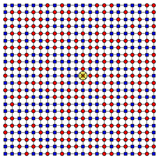
Grid Topologies. Aiming at a systematic approach, we consider three different grid topologies. Firstly, the Cayley tree grid, Fig. 1 a), resembles typical distribution grids which are preferably operated in such a tree-like fashion to pinpoint and repair failures more easily. Starting from a center, a constant number of branches grows outward in a given number of branching levels, each time with the same branching number ${b.}$ Hence, the tree grids are characterized by ${b}$ and the level ${l}$ of branching, the distance between neighbored nodes ${a}$ and the total number of nodes ${N.}$ An important characteristic of grids is the degree ${d_{i},}$ the number of links connecting node ${i}$ to any other node. The degree of this tree grid is ${d=b+1,}$ with the exception of the edge nodes, which have degree ${d=1.}$ Secondly, the square grid, Fig. 1 b). It is a simple meshed topology, used as basic model for transmission grids with their strict redundancy demand to guarantee continuing operation even when a single line fails (n-1 criterion). These square grids are characterized by the distance between neighbored nodes ${a,}$ the linear grid size ${L}$ and the number of nodes ${N=(L/a)^{2}.}$ Their degree is constant, ${d=4,}$ except at edges ( $d=3$ ) and corners ( $d=2$ ). Thirdly, we choose the German transmission grid, Fig. 1 c) as a real-world example with an irregular realistic topology, which is inhomogeneous and highly meshed. As reference for the German transmission grid, the open-source SciGRID dataset was used [9]. Excluding island nodes in it, the largest connected network of the four highest voltage levels, 400 kV, 380 kV, 220 kV as well as some 110 kV lines, was adopted as grid model. It comprises ${N=502}$ nodes and 673 links. It has a wide distribution of degree ${d_{i},}$ Fig. 2, with average degree ${\langle d_{i}\rangle=2.7}$ and typical degree ${d_{typ}=\sqrt{{d_{i}}^{2}}=4.1.}$ Excluding stubs, singly connected nodes, mostly due to the artifact that this data set does not include the transnational European grid, we get an average degree ${\langle d_{i}\rangle=3.5.}$

Dynamic AC Grid Model. 3-phasic alternating current (AC) electric grids can be modeled by active power balance equations [4, 5, 6, 10, 11, 12]. Since the three phases are typically loaded and operated symmetrically, they can effectively be reduced to a single phase. Furthermore, linking the grid nodes, purely inductive lines are assumed, neglecting the Ohmic losses along the lines, which are relatively small in high voltage transmission grids. The combined inductance of an individual 3-phasic line between nodes ${i}$ and ${j}$ is ${L_{ij}.}$ The line power capacity is then ${K_{ij}=|V_{i}||V_{j}|/(\omega L_{ij})}$ where ${V_{i},}$ ${V_{j}}$ are the voltages at node ${i}$ and ${j.}$ ${\omega}$ is related to the grid frequency ${f=50\mathrm{~Hz}}$ by ${\omega=2\pi f.}$ We will focus on the dynamics of the phases ${\varphi_{i},}$ while the voltage amplitudes are taken constant, since they typically change only on larger time scales. We assume the same voltage amplitude throughout the grid, so that ${V_{i}=V\exp(\T1\i\phi_{i})}$ with ${\phi_{i}}$ being the voltage phase. Since our main goal is to study the influence of the grid topology and the inertia on the phase dynamics we assumed that all links have equal inductance ${L}$ and thus equal power capacity ${K=V^{2}/(\omega L).}$ Thus, the power capacity linking nodes ${i}$ and ${j}$ is given by ${K_{ij}=KA_{ij},}$ where ${A_{ij}}$ is the adjacency matrix of the grid. Under these conditions, the stationary active power flow in the grid is obtained from Kirchhoff’s laws as function of the voltage phases ${\phi_{i}}$ as

with the second equation being the power balance condition, which has to be preserved at any time in order to avoid frequency shifts and is therefore controlled by grid operators. However, the nodal phases vary with time. The constant grid frequency gives a phase shift which increases linearly in time as ${\omega t,}$ independently of the node ${i.}$ Denoting the solution of the stationary balance equation Eq. (1) by the phase shift ${\theta_{i}^{0},}$ we can write

with the additional dynamic, time dependent phase shift denoted by ${\alpha_{i}(t).}$ In the present work all grid nodes are assumed to be connected to rotating machines, either synchronous generators or motors with inertia ${J_{i}.}$ All rotating machines and therefore all nodes are assigned an equal magnitude of electric power ${P,}$ which is either positive (generator) or negative (motor). Consequently, ${P_{i}=s_{i}P,}$ with ${s_{i}\in\{+,-\}}$ and ${J_{i}=J.}$ The phase dynamics is then governed by the balance of the change in kinetic energy, the energy dissipation in the machines, and the electrical energy exchange with adjacent grid nodes, yielding the swing equations [4, 5, 6].

where ${\gamma}$ is the damping constant and
${F_{ij}=K_{ij}\sin(\phi_{i}-\phi_{j})}$ is the power flow in the transmission line between nodes ${i}$ and ${j.}$

We note that, if the nodes would not be coupled by the transmission lines, the phase at each node would decay exponentially fast with the local relaxation time ${\tau=J/\gamma,}$ increasing with inertia ${J}$ and decreasing with damping parameter ${\gamma.}$ Therefore, when studying the effect of the coupling between the nodes, it is convenient to scale the time with relaxation time ${\tau.}$ In order to study the spreading of perturbations, the temporal and spatial dependence of ${\alpha_{i},}$ we insert Eq. (2) into Eq. (3) and for small phase velocities, ${\partial_{t}\alpha_{i}\ll\omega,}$ we arrive at the swing equations in dimensionless form,

with dimensionless parameters ${\Pi_{P}=JP/(\gamma^{2}\omega)}$ and ${\Pi_{K}=JK/(\gamma^{2}\omega).}$

Transient Dynamics. Now, we proceed to solve the nonlinear swing equations Eq. (4) on the different grid topologies shown in Fig. 1 for a set of parameters ${(\tau,\Pi_{K},\Pi_{P}),}$ in order to study the transient behavior of the AC grid when it is perturbed by a local disturbance.

As disturbance of the stationary state we increase the power for a short time interval ${0\leq t\leq\Delta t_{pert},}$ at the grid node marked with ‘x’ in the different grid topologies, Fig. 1. We choose it as one per mille of the initial power ${P,}$ corresponding to a perturbation energy ${E_{pert}^{0}=0.001\Pi_{P}\cdot\Delta t_{pert}.}$ The resulting transient behavior of the phase deviation ${\alpha(t)}$ is shown exemplary in Fig. 3 for the Cayley tree grid of Fig. 1 a) as function of rescaled time ${t^{*}=t/\tau}$ for the parameters ${(\Pi_{K}=10,\sigma=\Pi_{P}/\Pi_{K}=0.08).}$ We see that the phase at the disturbed node, ${r^{*}=0}$ (The distance between any two nodes ${r_{ij}}$ is defined as the number of edges in a shortest path connecting them [13]; ${r^{*}=r/a.}$ ) is perturbed first, reaching a maximum after a delay time, and then decaying in an oscillatory manner. As expected, phases of nodes further away from the origin of the disturbance are perturbed later and reach smaller amplitudes. We will analyze this temporal and spatial behavior quantitatively in the following.

Another way to visualize this transient behavior is the phase portrait shown exemplary in Fig. 4, a plot of phase velocity ${\dot{\alpha_{i}}}$ versus phase ${\alpha_{i}.}$ We see in the upper figure that the disturbance remains within the basin of attraction of the attractive fixed point for ${\Pi_{K}=100}$ and ${\sigma}$ not exceeding ${0.2.}$ There is a slight shift of the phase to which the perturbation decays at the end, which we find to be due to a global phase shift of all nodes induced by the disturbance at the center node. In the lower figure it is seen that the perturbation destabilizes the grid when ${\sigma=0.22,}$ where the phase deviation increases unbounded. Since we are interested in the propagation of small disturbances which do not destabilize the system, we review next the conditions for stability in order to choose the size of the disturbance accordingly.

Stability. Not all values of the parameters ${\Pi_{P}}$ and ${\Pi_{K}}$ allow for a stable stationary state. Without any disturbance, the criterion to distinguish between stable (allowed) and unstable (forbidden) parameters is the existence of a non-complex solution for the stationary state, Eq. (1). Thus, the ratio ${\sigma=\Pi_{P}/\Pi_{K}}$ determines whether parameters are allowed or forbidden and a critical value ${\sigma_{c}}$ exists depending on grid topology and power distribution. If the power distribution is ${P_{i}=s_{i}P,}$ with ${s_{i}\in\{+,-\},}$ and there are no clusters of consumers or clusters of generators, the critical value at node ${i}$ is given by ${\sigma_{ci}=d_{i},}$ where ${d_{i}}$ is the node degree. Thus, the critical value below which all nodes of the whole grid are stable is given by ${\sigma_{c}={\rm min}(d_{i}).}$ For a general distribution of ${P_{i},}$ there can be clusters of generators or consumers. Then, the critical value ${\sigma_{c}}$ is determined by the size and form of the clusters. If a cluster of generators has the total power ${P_{C}=\sum_{\rm cluster}P_{i},}$ with an effective degree ${d_{C},}$ as obtained by counting the number of consumers which are directly coupled to that cluster, the critical value of ${\sigma=\Pi_{Pi}/\Pi_{K}}$ above which no stable solution exists, is given by ${\sigma_{c}={\rm min}(P~d_{C}/P_{C}).}$

Depending on the magnitude of the disturbance it can destabilize the grid already at ${\sigma<\sigma_{c}.}$ In the Suppl. I. we derive a typical upper limit for the size of the perturbation ${\alpha}$ before it kicks the system out of the stable region. We find that the disturbance can destabilize the grid at smaller values ${\sigma^{*}(\alpha)<\sigma_{c}.}$ ${\sigma^{*}(\alpha)}$ coincides with ${\sigma_{c}}$ only in the limit, when the perturbation amplitude is vanishing, ${\sigma^{*}(\alpha\rightarrow 0)=\sigma_{c}.}$

Classification of Transient Dynamics: Parametric Phase Diagrams. Next, in order to analyze the transient behavior of disturbances we calculate the absolute values of the changes in power flow in the transmission line between nodes ${i}$ and ${j,}$
${\Delta F_{ij}(r)=|F_{ij}(r)-F_{ij}^{0}(r)|,}$ averaged over all transmission lines at a distance ${r}$ from the disturbance and divided by its maximum value,

In Figs. 5 we show examples for transient dynamics ${\Delta f}(r^{*},t^{*})$ in three grid topolgies for several different parameter values ${\Pi_{K},\sigma.}$ If there is no stable solution the phase perturbation increases without bound as seen in the example of Fig. 5 c) for the Cayley tree grid and in the lower phase portrait of Fig. 4. In order to find the parametric dependence systematically, we varied both parameters ${\Pi_{K}}$ and ${\sigma}$ in small steps. By mapping all parameters for which we find unstable solutions, we find unstable parameter regions for ${\sigma>\sigma_{c},}$ as shown in red in Fig. 6 a) for the tree grid, in Fig. 6 b) for the square grid with periodic arrangement, in Fig. 6 c) for the square grid with random arrangement of consumers and generators, and in Fig. 6 d) for the German transmission grid. The critical values of ${\sigma_{c}}$ depend on the grid topologies: For the Cayley tree grid with ${b=3}$ we find ${\sigma_{c}=0.2,}$ for the square grid with periodic arrangement ${\sigma_{c}=2.00,}$ for the Square grid with random arrangement ${\sigma_{c}=1.25}$ and for the German transmission grid ${\sigma_{c}=0.33.}$ In the stable regions we identify the following three qualitatively different transient behaviours:

The perturbation decays exponentially fast (FE) with local relaxation rate ${\Gamma_{0}}$ superimposed by oscillations, as seen in exemplary transients at the origin of the disturbance ${\Delta f(0,t^{*})}$ in Fig. 5 a) for tree grid, in Fig. 5 f) for periodic square grid, in Fig. 5 i) for random square grid and in Fig. 5 l) for German transmission grid. All parameter sets showing FE behavior are plotted in Fig. 6 a)-d) as green circles.

We observe the decay to be exponential with a smaller relaxation rate ${\Gamma<\Gamma_{0},}$ for a large interval of time ${t-t_{0}\gg\tau}$ as seen in Figs. 5 b) for the tree grid, e) and h) for the square grids and k) for the German grid. The corresponding parameter sets which show such slow exponential relaxation (SE) are shown in Fig. 6 a)-d) as yellow squares.

In the green shaded area fast relaxation (FE) is expected to occur according to analytical results of the next section, limited by the dashed lines in Fig. 6 a)-c), a plot of Eq. (12) for the tree grid and of Eq. (8) for the square grids, respectively. For the German grid, we indicate the boundary of that region in Fig. 6 d) by a dotted line, as suggested by numerical results. The yellow shaded areas in Fig. 6 a)-c) show where slow relaxation (SE) is expected to occur according to the analytical results. There is good agreement, the slight inconsistency is in a region where we observe deviations of ${\Gamma}$ from ${\Gamma_{0}}$ by only a few percent, well within the estimated errorbars of the numerical results. This parametric dependence of the relaxation rate is also seen in Fig. 7 for the ${b=3}$ Cayley tree grid where we plot the decay rate ${\Gamma(\sigma)}$ in units of local relaxation rate ${\Gamma_{0},}$ as obtained by fitting the transient behavior with an exponential decay.

Finally, and most surprisingly, we observe an even slower decay with a power law in time in square grids and in the German grid, as seen in exemplary plots Figs. 5 d) and g) for the square grids and j) for the German grid. The power is close to ${2,}$ in good agreement with diffusive behavior for ${\Delta f(t),}$ as obtained for a model square grid by an analytical derivation [8], see the next section, Eq. (34). Although that result was derived for square grids only, the numerical results indicate that such diffusive behavior may occur also in other meshed grids, as the example of the German grid shows at small values of the parameter ${\Pi_{K}<2,}$ Fig. 5 j). Thus, although the local relaxation time ${\tau=J/\gamma}$ decreases when the inertia ${J}$ is lowered, more nodes become correlated and thereby the spreading of a disturbance is slowed down to a collective diffusive spreading for times ${t>\tau}$ as ${\Pi_{K}}$ and thereby the inertia ${J}$ is lowered.

Diffusive propagation results also in a slowed spatial spreading of disturbances, as seen by calculating the expectation value of the squared distance, ${\langle r_{t}^{2}\rangle=\sum_{i}\alpha_{i}^{2}(t)(r_{i}-r_{j})^{2}/\sum_{i}\alpha_{i}^{2}(t).}$ Diffusion results in linear increase with time for times ${t-t_{0}>\tau,}$ while ballistic motion gives a faster, quadratic increase. In Fig. 8 b) the result is shown for a square grid with periodic arrangement of ${P_{i}.}$ We find that ${\langle r_{t}^{2}\rangle}$ increases initially very fast for times ${t-t_{0}<\tau.}$

For small ${\Pi_{K}=0.1}$ it slows down to a power law increase for ${t-t_{0}>\tau}$ with ${\langle r_{t}^{2}\rangle\sim t^{\beta},}$ where
${\beta=1.12}$ fits the data, which is a very strong indication of diffusive propagation in square grids with small inertia. Finally, the expectation value of the squared distance converges to a value of the order of the system area ${L^{2}}$ for large times ${t-t_{0}>1000\tau.}$ Arranging ${P_{i}}$ randomly, we find an even better agreement with diffusive behavior, ${\beta=1.01}$ for ${\Pi_{K}=0.1.}$ On the Cayley tree grid such a slow increase of ${\langle r_{t}^{2}\rangle}$ is absent, it reaches a value of the order of the system area much earlier. This is in agreement with our observation that diffusive power law decay is absent in the transients of tree like grids, Fig. 6 a). In the german transmission grid we find for the node marked by a cross in Fig. 1, that the squared distance ${\langle r_{t}^{2}\rangle}$ increases more slowly than in the square grid for ${\Pi_{K}=10,}$ see Fig. 8 d), in agreement with the insight that the spreading is slowed down in meshed grids. At smaller intertia, corresponding to ${\Pi_{K}=0.1,}$ it shows for that node a particular behavior with a delayed spreading followed by a faster spreading of the disturbance.

In the next section we present analytical results for the transient behavior for model grids. We show that diffusive spreading of disturbances, is possible in meshed grids like square grids, but that it is absent in tree like grids. This is traced to the presence of a spectral gap in the Laplace operator of these grids.

Spectral Analysis of Disturbances.

Periodic Square Lattice. For a square lattice where the power capacitance ${K}$ is the same for all transmission lines and generator and consumer power ${P_{i}=\pm P}$ is arranged periodically, an analytical solution is obtained with the plain wave Ansatz ${\phi_{qi}=c_{q}e^{\imath{\bf qr}_{i}}}$ where ${{\bf q}}$ is the wave vector. The Eigenfrequency ${\epsilon_{q_{n}},}$ is obtained as [8],

where ${\sigma/\sigma_{c}=P/(4K)}$ and
${f_{q_{n}}=2(\cos q_{nx}a+\cos q_{ny}a).}$ For finite size ${L,}$ the wave vectors are quantized, ${q_{x,yn}=n_{x,y}\pi/L,}$ with
${n_{x,y}=0,\pm 1,....}$ The resulting dispersion of the Eigenfrequency ${\epsilon_{q}}$ is plotted in Fig. 9 as function of the discrete wave number ${q_{n}}$ (blue dots). We observe a gap to the first excitation energy ${\epsilon_{q_{1}}=\Delta_{L}}$ as indicated by the dotted line in Fig. 9, which decreases with size ${L}$ as

Inserting ${\Lambda_{n}=\tau^{2}\epsilon_{q_{n}}^{2}}$ into the Fourier expansion Eq. (26), we get the transient behavior of the phase deviation ${\alpha(t)}$ for all times ${t.}$ The condition that slow modes with a small relaxation rate appear is, that the spectral gap ${\Delta_{L}}$ is smaller than the local relaxation rate, ${\Gamma_{0}.}$ This yields the parametric condition ${\Pi_{K}<\Pi_{K}^{S}(L),}$ where ${\Pi_{K}^{S}(L)}$ depends on grid size ${L}$ and ratio $\sigma$ as

This result is plotted in the phase diagram Fig. 6 b) (dashed line) together with numerical results. If the condition ${\Pi_{K}<\Pi_{K}^{S}(L)}$ is fulfilled, Eigenmodes with small wave number ${q}$ have purely imaginary ${\Omega_{q}}$ which results in slow decay of the deviation without oscillations. Summing over all slow modes in the spectral representation of ${\alpha_{i}(t),}$ Eq. (26) we find that a perturbation at node ${j}$ spreads for times ${t>\tau}$ and distances exceeding the mean free path ${l=v_{0}\tau}$ Thus, the initially localized perturbation spreads diffusively with diffusion constant ${D=v_{0}^{2}\tau/2,}$ with velocity ${v_{0}=\sqrt{\Pi_{K}\cos\delta_{0}}a/\tau,}$ see Suppl. III for the derivation. Diffusion causes slow power law relaxation of the disturbance at the initial site and an initial increase, followed by a power law decay at other sites. The resulting power law relaxation of the change in transmitted power between nodes ${k}$ and ${l}$ is [8]

Thus, we find analytically that the change in power at the site of the perturbation ${r_{\rm j}}$ decays with a power law in time with power ${2}$ in excellent agreement with the numerical results for the periodic square grid, Fig. 5 d). The expectation value of the square of the distance to the perturbation ${\langle r_{t}^{2}\rangle,}$ is for the diffusive propagation at times ${t>\tau,}$ Eq. (34) obtained to be ${\langle r_{t}^{2}\rangle=2Dt,}$ increasing linearly with time ${t.}$ After the Thouless time ${t_{L}=L^{2}/D}$ [17], the disturbance reaches the boundary of the grid and is reflected. Then, for times exceeding ${t_{L},}$ the disturbance decays exponentially with rate
$\Gamma_{min}=(1-(1-\tau^{2}\Delta^{2})^{1/2})\Gamma_{0}.$

For square grids with inhomogenous distribution of power ${P_{i}}$ slowly decaying modes appear when
${\Pi_{K}<\Pi_{K}^{s}(L),}$ with ${\Pi_{K}^{s}(L)}$ given by Eq. (8), where ${\sigma_{c}}$ is the critical value for that distribution of power ${P_{i}.}$ Diffusion occurs with an accordingly modified diffusion constant ${D.}$ We plot ${\Pi_{K}^{s}(L),}$ the dashed line in Fig. 6 c), together with numerical results where we use the numerically obtained value for ${\sigma_{c}.}$

Cayley Tree Grid. On a Cayley tree grid every inner node is connected to ${d=b+1}$ other nodes, as shown in Fig. 1 a) for ${b=3.}$ For the Cayley tree with branching ${b>1,}$ the symmetric eigenvectors were found only recently by Mahan in Ref. [18]. Inserting these Eigenvectors into the discrete wave equations Eq. (Methods) we obtain the Eigenfrequencies

For $b>1,$ ${q}$ can not be identified with a wave number since the phase of the Eigenvectors depends nonlinearly on ${qa.}$ We plot $\epsilon_{q}$ in Fig. 9 for a finite sized tree as function of discrete number ${q_{n}}.$ It is remarkable that Eigenfrequencies Eq. (10) have for ${b>1}$ a finite gap ${\Delta,}$ independent on the number of nodes ${N,}$

as indicated by the dashed line in Fig. 9. The condition that slow modes appear is ${\Delta<\Gamma_{0},}$ which yields the parametric condition ${\Pi_{K}<\Pi_{K}^{s},}$ with

If that condition is fulfilled, the perturbation decays for large times exponentially with a reduced relaxation rate $\Gamma_{min}=(1-(1-\tau^{2}\Delta(z,\Pi_{K})^{2})^{1/2})\Gamma_{0}$ which can be much smaller than the local relaxation rate ${\Gamma_{0}.}$ We plot ${\Pi_{K}^{s}(\sigma/\sigma_{c})}$ in Fig. 6 a) as the dashed line. For a tree grid with inhomogenous distribution of power ${P_{i},}$ typically, the slowly decaying modes are expected to appear when ${\Pi_{K}<\Pi_{K}^{s},}$ with ${\Pi_{K}^{s}}$ given by Eq. (12), where ${\sigma_{c}}$ is the critical value for that distribution of power ${P_{i}.}$

Discussions. For the german transmission grid the lines have a typical capacity of ${K_{ij}=10\text{ GW}}$ [9]. Assuming that half of the nodes act as generators and the other half as consumers to meet Germany’s peak power production of ${83\text{ GW}}$ [19], we set $|{P_{i}|=300\text{ MW}.}$ Typical conventional power plants of that rated power have inertia ${J=10^{4}\text{ kg m}^{2}}$ and damping ${\gamma\omega^{2}=0.10P.}This$ yields ${J\omega^{3}=310\text{ GW}},$ ${\Pi_{\rm P}=1.03\cdot 10^{5}}$ and ${\Pi_{\rm K}=3.44\cdot 10^{6}.}$ Taking the condition ${\Pi_{K}<\Pi_{K}^{S}(L),}$ with Eq. (12) as an estimate that meshed grids show diffusive behaviour, that condition becomes for currently existing transmission grids, ${L>1856a.}$ Thus, diffusive propagation is unlikely to occur in present transmission grids even on the European scale. However, as conventional power plants become substituted by renewable energy the inertia in the grid becomes reduced substantially [1]. Thus, the dynamics of transmission grids changes. For small inertia of ${J=0.1\text{ kg m}^{2}}$ and otherwise same parameters, we find ${\Pi_{\rm P}=1.03}$ and ${\Pi_{\rm K}=34.45}$ so that the condition to observe diffusion is ${L>5.87a}$ and becomes relevant for transmission grids on the national scale. If no measures are undertaken to substitute the inertia of conventional power plants[20], we conclude that transient dynamics will change drastically, disturbances relaxing slowly and spreading by collective diffusive propagation.

In conclusion, we studied how the relaxation and propagation of disturbances in AC grids is modified when system parameters like the inertia in the grid are changed. To this end we solved the nonlinear swing equations on three different grid topologies numerically and analyzed the results comparing them quantitatively with analytical insights obtained by mapping the swing equations for small perturbations on discrete wave equations. We solved these wave equations by generalized Fourier expansion for the square grid and the Cayley tree grid. Thereby we show that the long time transient behavior is governed by the spectral gap between the stationary state and the lowest Eigenmode of its grid. While the Cayley tree grid has a finite spectral gap, independent on grid size, meshed grids have a small spectral gap which is reduced strongly with increasing grid size, leading to slowed relaxation and collective diffusive propagation of disturbances. Analyzing the numerical results we confirm that, depending on inertia, geographical distribution of power, grid power capacity and topology, the disturbance may either decay exponentially in time with the decay rate of a single node, ${\Gamma^{0},}$ or exponentially with a smaller decay rate ${\Gamma<\Gamma^{0},}$ or, even more slowly, decaying with a power law in time, resulting in collective diffusive propagation. Such slow decay of disturbances could be prevented by avoiding meshed grids in favour of tree like grids.

Stationary solution. Before any perturbation is applied, we calculate the stationary state ${\theta_{i}^{0}}$ at every node ${i}$ in the grid. This is accomplished by first obtaining an analytical solution of Eq. (1) for small phase differences linearizing ${\sin(\theta^{0}_{i}-\theta^{0}_{j})\rightarrow\theta^{0}_{i}-\theta^{0}_{j}.}$ Thereby Eq. (1) can be rewritten by introducing the weighted graph Laplacian matrix
${H_{ij}=-K_{ij}+\delta_{ij}\sum_{l}K_{il},}$ as

where ${{\bf P}}$ and ${\mbox{\boldmath$\theta$ }^{0}}$ are vectors, whose ${i}$ -th component is the power and stationary phase at node ${i,}$ respectively. ${H}$ has at least one zero Eigenvalue. Therefore, we need to calculate the pseudo inverse ${H^{+},}$ yielding ${\mbox{\boldmath$\theta$ }^{0}=H^{+}\cdot{\bf P}.}$ We use this numerical solution then as initial condition for a numerical root solver to find the solution of the nonlinear equation, Eq. (1). This way, the numerical accuracy of the stationary solution is maximized which is important, since we use it as initial condition for the swing equation to make sure that we start in stationary conditions.

Numerical Solution of Swing Equations. Having found the stationary phases ${\theta_{i}^{0}}$ as solutions of the stationary state equations Eq. (1), we can insert them into the swing equations Eq. (4). Next, we solve these equations to study the transient bahavior when the AC grid is perturbed by a local disturbance as outlined in detail in Suppl. I. We study the transient phase deviation ${\alpha_{i}}$ and the phase velocity ${\partial_{t}\alpha_{i},}$ as well as the change in transmitted power between all connected nodes ${i,j,}$ ${\Delta F_{i,j}.}$ In this article, we are primarily interested to understand the propagation of disturbances which are so small that they do not destabilize the grid.

Analytical Derivation. For small perturbations, corresponding to the parametric condition ${\sigma<\sigma^{*}(\alpha),}$ we can analyse the swing equations Eq. (4) by expanding it in the perturbation ${\alpha_{i}-\alpha_{j}.}$ This yields the linear wave equations on the grid [8],

with coupling amplitudes ${t_{ij}=\Pi_{Kij}\cos(\theta^{0}_{i}-\theta^{0}_{j}),}$ depending both on grid topology and on the initial distribution of power ${P_{i}}$ through the stationary phases ${\theta^{0}_{i}.}$ These coupling amplitudes ${t_{ij}}$ form the generalized Laplace operator ${\Lambda}$ with ${\Lambda_{ij}=-t_{ij}}$ and
${\Lambda_{ii}=\sum_{i}t_{ii},}$ which is related to the stability matrix in the linear stability analysis [14, 15]. The dimensionless disturbance function is defined by
${\delta\Pi_{i}(t)=J\delta P_{i}(t)/(\gamma^{2}\omega).}$ We expand the phase deviation ${\alpha_{i}(t)}$ and the disturbance ${\delta\Pi_{i}(t)}$ in a generalized Fourier series in terms of the Eigenvectors ${{\bf\phi}_{n}}$ of ${\Lambda,}$ as defined by ${\Lambda{\bf\phi}_{n}=\Lambda_{n}{\bf\phi}_{n},}$ where ${\Lambda_{n}}$ is its Eigenvalue [8, 16, 15, 14], see Suppl. III for a detailed derivation. For a local perturbation at a site ${j,}$ lasting only a short time interval ${\Delta t\ll\tau}$ around time ${t_{0},}$ ${\delta\Pi_{i}(t)=\delta\Pi\delta_{ij}\tau\delta(t-t_{0}),}$ we find

where ${\Omega_{n\pm}=-\T1\i(1\pm\sqrt{1-\Lambda_{n}})1/\tau.}$ In order to find the transient dynamics for all times ${t,}$ it remains to find the Eigenvalues ${\Lambda_{n}\epsilon_{n}^{2}\tau^{2}}$ and Eigenvector components ${\phi_{ni},}$ as can be done numerically for arbitrary grids. For particular grids, analytical solutions can be obtained as we reviewed above and in Suppl. III.

We gratefully acknowledge the support of BMBF in the frame of CoNDyNet FK. 03SF0472D.

More information on methods and derivations is provided in the appended supplementary text. For further illustration we also provide three exemplary movies showing the propagation of disturbances in a tree grid, a square grid and the german transmission grid.

Research design and numerics were performed by S.T and M.C., with S.K. supervising the project and performing the analytical calculations. All authors contributed to editing the manuscript.

The authors declare no competing financial interests.

References

- [1] Ulbig, A., Borsche, T. S. & Andersson, G. Impact of low rotational inertia on power system stability and operation. IFAC Proceedings Volumes 14(3), 7290-7297 (2014).
- [2] Kundur, P. Power System Stability and Control. (Mc Graw Hill, 1994).
- [3] Machowski, J., Bialek, J.W. & Bumby, J.R. Power System Dynamics: Stability and Control. (Wiley, 2008).
- [4] Bergen, A.R. & Hill, D.J. A structure preserving model for power system stability analysis. IEEE Trans. on Power App. and Syst. 100(1), 25-35 (1981).
- [5] Filatrella, G., Nielsen, A.H. & Pedersen, N.F. Analysis of a power grid using a Kuramoto-like model. Eur Phys. J. B 61(4), 485-491 (2008).
- [6] Rohden, M., Sorge, A., Timme, M. & Witthaut, D. Self-organized synchronization in decentralized power grids. Phys. Rev. Lett. 109, 064101 (2012).
- [7] Schmietendorf, K., Peinke, J., Friedrich, R. & Kamps, R.O. Self-organized synchronization and voltage stability in networks of synchronous machines. Eur. Phys. J. Spec. Top. 223(12), 2577-2592 (2014).
- [8] Kettemann, S. Delocalization of disturbances and the stability of AC electricity grids. Phys. Rev. E 94, 062311 (2016).
- [9] Matke, C., Medjroubi, W. & Kleinhans, D. SciGRID - An Open Source Reference Model for the European Transmission Network (v0.2), (July 2016).
- [10] Heuck, K., Dettmann, K.D. & Schulz, D. Elekrtische Energieversorgung, 9th edition. (Springer, 2009).
- [11] Rohden, M. Self-organized Synchronization in Decentralized Power Grids. PhD thesis, (Göttingen, 2014).
- [12] Menck, P.J., Heitzig, J., Kurths, J., & Schellnhuber, H.J. How dead ends undermine power grid stability. Nature Communications 5, 3969 (2014).
- [13] M. Newman, Networks: An Introduction. (OUP, Oxford, 2009).
- [14] Coletta, T. & Jacquod, P. Linear stability and the Braess paradox in coupled-oscillator networks and electric power grids. Phys Rev E 93, 032222 (2016).
- [15] Nishikawa, T. & Motter, A.E. Comparative analysis of existing models for power grid synchronization. New J. Phys. 17, 015012 (2015).
- [16] L. A. Torres-Sánchez, G. T. Freitas de Abreu, S. Kettemann, Analysis of the Dynamics and Topology Dependencies of Small Perturbations in Electric Transmission Grids, subm. to IEEE Power Systems, arXiv:1706.10130 (2017).
- [17] Edwards, J.T. & Thouless, D.J. Numerical studies of localization in disordered systems. J. Phys. C: Solid State Phys. 5, 807 (1972).
- [18] Mahan, G.D. Energy bands of the Bethe lattice. Phys. Rev. B 63, 155110 (2001).
- [19] Bayer, E. Report on the German Power System, Country Profile 057/03-CP-2014/EN, Agora Energiewende. (Berlin, Germany, 2015).
- [20] T. Borsche and F. Dörfler, On Placement of Synthetic Inertia with Explicit Time-Domain Constraints, subm to IEEE Transactions on Power Systems, https://arxiv.org/abs/1705.03244 (2017).
- [21] E. Kreyszig, Advanced Engineering Mathematics, 9th edition., Wiley, New York (2006).
Supplementary
Appendix I Numerical Simulations
We employ a standard differential equation solver, the Runge-Kutta algorithm [21] using the commercial software MATLAB®. Since this is a shooting method its convergence is improved considerably by setting the phases to the stationary state solutions before the perturbation. The perturbation is applied at . Calculated time spans prior and past perturbation were iteratively adjusted to ensure both a stationary state onto which the perturbation is applied and to capture the whole perturbation event until complete decay. Temporal resolution was chosen fine enough to avoid undersampling of the oscillating phases using the phase portraits as sensors. They would show smooth curves for sufficient resolution or angled curves for too poor resolution. In favour of automatized calculation, time span and resolution were mostly not adapted but rather chosen better than necessary. Concretely, for German and square grid, throughout all values of , in steps of . For the Cayley tree grid, time span and resolution were i) in steps of for and ii) in steps of for .
Appendix II Stability