Saturation of entropy production in quantum many-body systems

In the mid-nineteenth century, Rudolf Clausius introduced entropy as a measure of thermodynamic irreversibility, by arguing that, while the energy of the universe is constant, the entropy of the universe tends to a maximum [1]. Ever since, understanding inevitable irreversibility in the macroscopic world is one of the most fundamental problems in statistical physics. Especially, in light of the fact that isolated quantum systems have reversible dynamics, it has not been clear whether such a behavior of the entropy production is consistent with quantum theory.

From the modern point of view, thermalization of isolated quantum systems has been of much interest in light of state-of-the-art technologies such as ultracold atoms [2, 3, 4, 5, 6, 7], trapped ions [8], and superconducting qubits [9]. For example, it has been established that even a pure quantum state in an isolated system exhibits relaxation toward thermal equilibrium by unitary dynamics [10, 11, 12, 13, 14, 15, 16, 17, 18, 19, 20, 21, 22, 23, 24]. Several key theoretical ideas have been developed to understand such relaxation processes. It has been rigorously proved that an overwhelming majority of pure states in the Hilbert space describe thermal equilibrium, which is referred to as typicality [25, 26, 27, 28]. The eigenstate thermalization hypothesis (ETH) is another cornerstone to understand thermalization [11, 13, 29, 30, 31, 32, 33, 34, 35, 36], which states that all the energy eigenstates in an energy shell are thermal. The ETH (or the strong ETH) is believed to be true for non-integrable systems without disorder. We note that there is a weaker version of the ETH (the weak ETH) [33], which states that most of the energy eigenstate are thermal. The weak ETH is rigorously proved for both integrable and non-integrable systems without disorder [37, 38].

On the other hand, research into the second law, such as the fluctuation theorem [39, 40, 41, 42, 43, 44, 45, 46, 47, 48] and thermodynamic resource theories [49, 50], is based on a special assumption that the initial state of a heat bath is the canonical ensemble. This assumption is very strong, given that a thermal equilibrium state can even be a pure quantum state. If we do not assume the initial canonical distribution, the non-negativity of the entropy production cannot be proved by the conventional arguments, i.e., the fluctuation theorem or the positivity of relative entropy [46]. In this sense, except for only a few seminal works [51, 52, 53], the foundation of the second law in isolated quantum systems has not been fully addressed.

In this paper, we rigorously prove that the entropy production saturates at some value in the long time regime, for a broad class of initial states including pure states. We note that the entropy production, the sum of the change in von Neumann entropy of a subsystem and the heat absorbed from a heat bath, can change in time, though the von Neumann entropy of the total system is invariant under unitary dynamics [54]. In general, the saturation value of the entropy production depends on both the initial state and the Hamiltonian, and could be negative. We then prove that the saturation value is non-negative if the system satisfies the strong ETH, which leads to the second law of thermodynamics in the long time regime. Our results provide a quantum foundation to observation by Clausius.

We note that in our previous work [38], we have proved the second law for pure quantum states in the short time regime, on the basis of the Lieb-Robinson bound [55, 56, 57]. However, the previous result cannot apply to the long time regime. In the present work, we have adopted a completely different technique from the Lieb-Robinson bound, and have proved the second law in the long time regime (see Fig. 1).

The rest of this paper is organized as follows. In Sec. II, we formulate our setup and make a brief review on equilibration in isolated quantum systems. In Sec. III, we prove the main theorem, which states that the entropy production takes a constant value for most times. In Sec. IV, we derive a lower bound of the saturation value of the entropy production. We also show that the saturation value is non-negative if the system satisfies the ETH. In Sec. V, we confirm our theory by numerical simulation of hard-core bosons. In Sec. VI, we summarize our results. In Appendix A, we make a remark on the effective dimension.

We consider a quantum many-body system described by a finite-dimensional Hilbert space. The total system is divided into two parts, a small system ${\mathrm{S}}$ and a large heat bath ${\mathrm{B}}$. Their Hilbert space dimensions are denoted by $D_{\mathrm{S}}$ and $D_{\mathrm{B}}$, respectively. The total Hamiltonian is given by

where $H_{\mathrm{S}}$ is the Hamiltonian of system ${\mathrm{S}}$, $H_{\mathrm{B}}$ is the Hamiltonian of bath ${\mathrm{B}}$, and $H_{\mathrm{I}}$ is the interaction between system ${\mathrm{S}}$ and bath ${\mathrm{B}}$. We write the spectrum decomposition of $H$ as

where $E_{j}$ is an eigen-energy ($E_{i}\neq E_{j}$ for $i\neq j$), and $P_{j}$ is the projector onto the eigenspace of $H$ with energy eigenvalue $E_{j}$.

We assume that the initial correlation between system ${\mathrm{S}}$ and bath ${\mathrm{B}}$ is zero. The initial density operator of the total system is then given by

where $\rho_{\mathrm{S}}(0)$ and $\rho_{\mathrm{B}}(0)$ are respectively the initial density operators of system ${\mathrm{S}}$ and bath ${\mathrm{B}}$. We do not assume that $\rho_{\mathrm{B}}(0)$ is the canonical ensemble.

The total system obeys the unitary time evolution generated by the total Hamiltonian $H$. The state at time $t$ is written by $\rho(t)=e^{-iHt}\rho(0)e^{iHt}$. Note that we set $\hbar=1$. We also write the time-averaged state by

which is called the diagonal ensemble. Because of the recurrence property of the unitary evolution, an isolated quantum system cannot converge to an exact stationary state. However, a system can relax to an effective stationary state most of the time between recurrences. In fact, it has been proved in Refs. [15, 58] that for any operator $O$, and for any $\epsilon>0$,

Here, $\mathrm{Prob}_{t\in[0,\tau]}$ is the uniform measure over $t\in[0,\tau]$, and $\left\|O\right\|$ is the operator norm of $O$. $D_{\mathrm{G}}$ is the degeneracy of the most degenerate energy gap, which is given by $D_{\mathrm{G}}:=\max_{j\neq k}\left|\{(l,m):G_{(l,m)}=G_{(j,k)}\}\right|$ with $G_{(j,k)}:=E_{j}-E_{k}$. If the total Hamiltonian $H$ has no degenerate energy gap, $D_{\mathrm{G}}=1$. $D_{\mathrm{eff}}$ is the effective dimension of the initial state $\rho(0)$, which is defined as $D_{\mathrm{eff}}:=1/\sum_{j}(\mathrm{Tr}[P_{j}\rho(0)])^{2}$. If the Hamiltonian has no degeneracy, the effective dimension is equal to the inverse of the purity of the diagonal ensemble, i.e., $1/\mathrm{Tr}[\omega^{2}]$. Inequality (5) means that observables equilibrate to their diagonal ensemble averages if $D_{\mathrm{eff}}$ is sufficiently large.

To quantify the distance between two density operators, we use the trace distance $\mathcal{D}(\rho,\tau):=\frac{1}{2}\mathrm{Tr}[\sqrt{(\rho-\tau)^{2}}]$. When it is small, we hardly distinguish two states. We also use the local distance $\mathcal{D}_{{\mathrm{S}}}(\rho,\tau):=\mathcal{D}(\rho_{\mathrm{S}},\tau_{{\mathrm{S}}})$, where we write $\rho_{\mathrm{S}}:=\mathrm{Tr}_{\mathrm{B}}[\rho]$ for the reduced density operator. We regard that system ${\mathrm{S}}$ equilibrates to the diagonal ensemble when the local distance $\mathcal{D}_{{\mathrm{S}}}(\rho(t),\omega)$ is small most of the time. It has been shown in Refs. [15, 58] that for any positive number $\epsilon>0$,

This inequality implies that system ${\mathrm{S}}$ equilibrates to the diagonal ensemble if $D_{\mathrm{eff}}$ is sufficiently large compared to the Hilbert space dimension of system ${\mathrm{S}}$.

The effective dimension $D_{\mathrm{eff}}$ of the initial product state $\rho(0)$ is bounded from below by the purity of the initial state of bath ${\mathrm{B}}$:

where $D_{\mathrm{E}}$ is the maximum energy degeneracy of the total Hamiltonian $H$. The proof of inequality (7) is the following. We denote by $K_{j}$ an orthonormal basis of the degenerate eigenspace of energy $E_{j}$. Then, we have

where we used $\mathrm{Tr}[\rho_{\mathrm{S}}(0)^{2}]\leq 1$ to obtain the last line.

When the initial state of bath ${\mathrm{B}}$ is the microcanonical ensemble $\rho^{\mathrm{mc}}_{\mathrm{B}}:=P_{{\mathrm{B}}}^{\mathrm{mc}}/\mathrm{Tr}[P_{{\mathrm{B}}}^{\mathrm{mc}}]$, where $P_{{\mathrm{B}}}^{\mathrm{mc}}$ is the projector onto the Hilbert space of the energy shell $M_{U,\Delta}=\{E^{{\mathrm{B}}}_{j}:\left|E^{{\mathrm{B}}}_{j}-U\right|\leq\Delta\}$ with $\Delta>0$ (see Sec. IV.2 for more details), or the canonical ensemble $\rho^{\mathrm{can}}_{\mathrm{B}}:=e^{-\beta H_{\mathrm{B}}}/\mathrm{Tr}[e^{-\beta H_{\mathrm{B}}}]$, then the purity $\mathrm{Tr}[\rho_{\mathrm{B}}(0)^{2}]$ is exponentially small in the size of bath ${\mathrm{B}}$ (see Appendix A). Thus $D_{\mathrm{eff}}$ is exponentially large in the size of bath ${\mathrm{B}}$. Furthermore, when the initial state of bath ${\mathrm{B}}$ is randomly taken from the Hilbert space of the energy shell according to the Haar measure, $D_{\mathrm{eff}}$ typically becomes exponentially large in the size of bath ${\mathrm{B}}$ (see again Appendix A). Therefore, system ${\mathrm{S}}$ equilibrates to the diagonal ensemble if the initial state of bath ${\mathrm{B}}$ is the microcanonical ensemble, the canonical ensemble, or a typical pure state, given that bath ${\mathrm{B}}$ is sufficiently large.

Finally, we define the entropy production from time $0$ to $t$ by

where $\Delta S_{{\mathrm{S}}}(t):=S_{{\mathrm{S}}}(t)-S_{{\mathrm{S}}}(0)$ is the change in the von Neumann entropy of system ${\mathrm{S}}$ with $S_{{\mathrm{S}}}(t):=S(\rho_{\mathrm{S}}(t))=-\mathrm{Tr}_{{\mathrm{S}}}[\rho_{\mathrm{S}}(t)\log\rho_{\mathrm{S}}(t)]$, and $Q(t):=-\mathrm{Tr}_{{\mathrm{B}}}[H_{\mathrm{B}}(\rho_{\mathrm{B}}(t)-\rho_{\mathrm{B}}(0)]$ is the heat absorbed by system ${\mathrm{S}}$. If the initial state of bath ${\mathrm{B}}$ is the canonical ensemble $\rho_{\mathrm{B}}(0)=\rho^{\mathrm{can}}_{\mathrm{B}}$, the entropy production $\langle\sigma(t)\rangle$ is always non-negative: $\langle\sigma(t)\rangle\geq 0$ [46], which is an expression of the second law of thermodynamics. This inequality results from the non-negativity of the quantum relative entropy. When the initial state of bath ${\mathrm{B}}$ is not the canonical ensemble, the entropy production $\langle\sigma(t)\rangle$ is not necessarily non-negative. In this paper, we discuss the behavior of the entropy production and the validity of the second law for general initial states.

In this section, we discuss our main topic: saturation of the entropy production under reversible unitary dynamics. In Sec. II, we discussed that system ${\mathrm{S}}$ equilibrates to the diagonal ensemble if the effective dimension is sufficiently large, i.e., inequalities (5) and (6). However, the entropy production cannot be described as the expectation value of any instantaneous observable. Therefore, we cannot directly apply the argument in Sec. II to the entropy production. Instead, we evaluate the difference between the entropy production at time $t$ and the saturated entropy production $\langle\sigma_{\infty}\rangle$ by using inequalities (5) and (6).

We now formulate our theorem rigorously. We assume that the initial state of the total system is given by a product state (3). The saturated entropy production $\langle\sigma_{\infty}\rangle$ is defined as

where $\omega$ is defined in Eq. (4), and $\omega_{{\mathrm{S}}}:=\mathrm{Tr}_{\mathrm{B}}[\omega]$. If the difference $\left|\langle\sigma(t)\rangle-\langle\sigma_{\infty}\rangle\right|$ is small most of the time, the entropy production saturates at $\langle\sigma_{\infty}\rangle$. In fact, we show the following theorem.

We have made no assumption on the initial state of bath $\mathrm{B}$; Theorem 1 is applicable not only to the canonical ensemble, but also to an arbitrary initial state. From Theorem 1 we find that a sufficient condition of the saturation is just the large effective dimension of the initial state. As we remarked in Sec. II, the effective dimension is exponentially large with the size of bath $\mathrm{B}$, when the initial state of bath $\mathrm{B}$ is the microcanonical ensemble, the canonical ensemble, or a typical quantum state. From Theorem 1, the entropy production saturates at $\langle\sigma_{\infty}\rangle$ for these cases.

We remark that the time scale, which makes the long time limit in Theorem 1 meaningful, is expected to be doubly exponentially large with respect to the size of the total system for non-integrable systems. This is much longer than the time scale determined by the Lieb-Robinson bound. However, it has been observed numerically and analytically that the informational quantities, such as the entanglement entropy, ballistically spread and saturate at around the Lieb-Robinson time for both of integrable and non-integrable systems  [60, 61, 62, 63]. As a result, the entropy production, defined with the von Neumann entropy, is expected to relax to the long-time average at around the Lieb-Robinson time, as numerically observed in Ref. [38] and also in Sec. V. Therefore, we expect that in practical situations, there is no intermediate time regime between the saturation of the entropy production and the Lieb-Robinson time. However, for the moment, it seems to be formidably difficult to prove it rigorously for general situations.

As mentioned before, it has been shown that the entropy production is always non-negative when the initial state of bath $\mathrm{B}$ is the canonical ensemble [46]. In this case, the entropy production increases and saturates at a non-negative value, which is consistent with the second law of thermodynamics.

On the other hand, the saturation value $\langle\sigma_{\infty}\rangle$ is not necessarily non-negative for a general initial state. In fact, $\langle\sigma_{\infty}\rangle$ is determined by the diagonal ensemble $\omega$, which in general depends on the details of the initial state. For this reason, it is difficult to prove the non-negativity of $\langle\sigma_{\infty}\rangle$ for completely general situations.

If the total system satisfies the strong ETH, $\omega_{{\mathrm{S}}}$ does not depend on the details of the initial state, but only depends on the initial average energy. We note that the strong ETH is believed to be true for non-integrable systems [13, 33, 34, 35, 36] (see also [24] for definitions of integrability in quantum systems). In such a case, the diagonal ensemble $\omega_{{\mathrm{S}}}$ of a general initial state is the same as that of the initial canonical ensemble, and therefore $\langle\sigma_{\infty}\rangle$ takes the same value as the canonical case, where $\langle\sigma_{\infty}\rangle$ is non-negative. This is the scenario that we will prove in the next section by assuming the strong ETH.

We now discuss the non-negativity of the saturated entropy $\langle\sigma_{\infty}\rangle$. Specifically, we utilize the ETH [11, 13, 29, 30, 31, 32, 33, 34, 35, 36], which is sufficient to show the non-negativity of $\langle\sigma_{\infty}\rangle$.

In Sec. IV.1, we prove a general lower bound of $\langle\sigma_{\infty}\rangle$ without using the ETH. Then, in Sec. IV.2, we show that the lower bound approaches to zero in the large bath limit, if the system satisfies the strong ETH. In Sec. IV.3, we discuss consequences of the weak ETH.

To confirm the validity of our theory, we performed a numerical simulation by using exact diagonalization. As a non-integrable model, we consider a one-dimensional hard-core bosons with nearest- and next-nearest-neighbor hoppings and interactions, which satisfies the strong ETH [34]. System $\mathrm{S}$ is a single site and bath $\mathrm{B}$ consists of $L$ sites. The annihilation (creation) operator of a hard-core boson at site $i$ is written as $c_{i}$ ($c_{i}^{\dagger}$), which satisfies the commutation relations $[c_{i},c_{j}]=[c_{i},c_{j}^{\dagger}]=[c_{i}^{\dagger},c_{j}^{\dagger}]=0$ for $i\neq j$, $\{c_{i},c_{i}\}=\{c^{\dagger}_{i},c_{i}^{\dagger}\}=0$, and $\{c_{i},c_{i}^{\dagger}\}=1$. The Hamiltonians are then given by

where $\omega>0$ is the on-site potential, $-\gamma_{\mathrm{I}}$ is the hopping rate between system $\mathrm{S}$ and bath $\mathrm{B}$, $-\gamma$ and $-\gamma^{\prime}$ are the hopping rates in bath $\mathrm{B}$, and $g>0$ and $g^{\prime}>0$ are the repulsion energies. We assume the open boundary condition. We note that $[H_{\mathrm{S}}+H_{\mathrm{B}},H_{\mathrm{I}}]\neq 0$ in this model. We set the initial number of bosons in bath ${\mathrm{B}}$ by $N_{\mathrm{b}}$. The initial state is a product state of system ${\mathrm{S}}$ and bath ${\mathrm{B}}$, where the state of system $\mathrm{S}$ is given as $|1\rangle:=c_{0}^{\dagger}|0\rangle$, and the state of bath ${\mathrm{B}}$ is an energy eigenstate $|E^{{\mathrm{B}}}_{j}\rangle$.

Figure 3 shows $D_{\mathrm{eff}}$ of the initial state $|1\rangle|E^{{\mathrm{B}}}_{j}\rangle$, which implies that $D_{\mathrm{eff}}$ increases with $L$ at all energy scales. We note that an energy eigenstate $|E^{{\mathrm{B}}}_{j}\rangle$ is not necessarily typical in the Hilbert space of the energy shell, and the amount of $D_{\mathrm{eff}}$ is nontrivial. The numerical result in Fig. 3 suggests that fluctuations of observables around the diagonal ensemble averages are negligible, and the entropy production will indeed saturate.

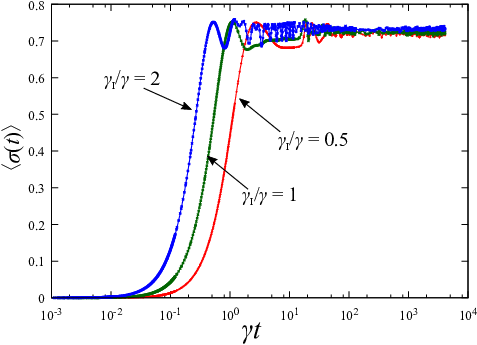
Figure 4 shows the time dependence of the entropy production. We set the inverse temperature as $\beta=0.1$, and choose an energy eigenstate $|E^{{\mathrm{B}}}_{j}\rangle$ such that its inverse temperature is closest to $0.1$ in the energy shell. Here, the inverse temperature $\beta$ of $|E^{{\mathrm{B}}}_{j}\rangle$ is given by the solution of $\mathrm{Tr}_{\mathrm{B}}[H_{\mathrm{B}}|E^{{\mathrm{B}}}_{j}\rangle\langle E^{{\mathrm{B}}}_{j}|]=\mathrm{Tr}_{\mathrm{B}}[H_{\mathrm{B}}\rho^{\mathrm{can}}_{\mathrm{B}}(\beta)]$. We set parameters as $L=16,\epsilon/\gamma=1,\gamma_{\mathrm{I}}/\gamma=1,g/\gamma=0.1,\gamma^{\prime}/\gamma=0.2,g^{\prime}/\gamma=0.1$, and $\gamma_{\mathrm{I}}/\gamma=0.5,1$, or $2$.

As shown in Fig. 4, the entropy production gradually increases up to $\gamma t\simeq 10^{0}$, oscillates in the medium regime $10^{0}\lesssim\gamma t\lesssim 10^{2}$, and then saturates in the long time regime $\gamma t\gtrsim 10^{2}$. This behavior is consistent with Theorem 1. The saturation value in the long time regime is positive for all the cases of $\gamma_{\mathrm{I}}/\gamma=0.5,1,2$. This implies that the error term in Theorem 3 is negligible in this example. The error term is also small in a two dimensional hard-core bosons with nearest-neighbor repulsion [38].

We note that the saturation value is independent of the interaction rate, which implies that the interaction strength affects the entropy production only in the short time regime. The entropy production is also non-negative in the short time regime, which is out of the scope of the present theory, but can be explained by our previous theorem based on the Lieb-Robinson bound [38].

In this paper, we have discussed the second law of thermodynamics for general quantum states in the long time regime. We have proved Theorem 1, which states that the entropy production saturates for most times [inequality (16)]. The saturation value (15) is given by the entropy production with respect to the diagonal ensemble $\omega$. We have then derived the lower bound (22) of the saturated entropy production. If the diagonal ensemble is independent of the parameters of the initial state except for the average energy, the obtained bound (22) implies the non-negativity of the saturated entropy production. This scenario can be justified by assuming the ETH. We have shown the initial state independence (Lemma 1) and the non-negativity of the saturation value (Theorem 3) under the strong ETH (Assumption 1) and an additional assumption on the initial energy (Assumption 2). We have also shown the non-negativity from the weak ETH (Theorem 4).

Our results have clarified that thermodynamic irreversibility can emerge from unitary dynamics of quantum many-body systems in the long time regime. We emphasize that, if the initial state of the bath is a pure state, the fluctuation theorem holds only in the short time regime, but breaks down in the long time regime [38]. This is because non-thermal quantum fluctuations of the initial state affect higher-order fluctuations of the entropy production in the long time regime. In contrast, as shown in the present work, the second law is robust in the long time regime, because the second law only concerns the first cumulant (i.e., the average) of the entropy production. More detailed investigation of the time scale of saturation of the entropy production is a future issue.

References

- [1] R Clausius, Mechanical Theory of Heat, with its Applications to the Steam-Engine to the Physical Properties of Bodies (J. Van Voorst, London, 1867).
- [2] Toshiya Kinoshita, Trevor Wenger, and David S. Weiss, “A quantum Newton’s cradle,” Nature 440, 900–903 (2006).
- [3] S. Hofferberth, I. Lesanovsky, B. Fischer, T. Schumm, and J. Schmiedmayer, “Non-equilibrium coherence dynamics in one-dimensional Bose gases,” Nature 449, 324–327 (2007).
- [4] Stefan Trotzky, Yu-Ao Chen, Andreas Flesch, Ian P. McCulloch, Ulrich Schollwöck, Jens Eisert, and Immanuel Bloch, “Probing the relaxation towards equilibrium in an isolated strongly correlated 1D Bose gas,” Nat. Phys. 8, 325–330 (2012).
- [5] M. Gring, M. Kuhnert, T. Langen, T. Kitagawa, B. Rauer, M. Schreitl, I. Mazets, D. A. Smith, E. Demler, and J. Schmiedmayer, “Relaxation and Prethermalization in an Isolated Quantum System,” Science 337, 1318–1322 (2012).
- [6] T. Langen, R. Geiger, M. Kuhnert, B. Rauer, and J. Schmiedmayer, “Local emergence of thermal correlations in an isolated quantum many-body system,” Nat. Phys. 9, 640–643 (2013).
- [7] Adam. M. Kaufman, M. Eric Tai, Alexander Lukin, Matthew Rispoli, Robert Schittko, Philipp M. Preiss, and Markus Greiner, “Quantum thermalization through entanglement in an isolated many-body system,” Science. 353, 797 (2016).
- [8] Govinda Clos, Diego Porras, Ulrich Warring, and Tobias Schaetz, “Time-Resolved Observation of Thermalization in an Isolated Quantum System,” Phys. Rev. Lett. 117, 170401 (2016).
- [9] C. Neill, P. Roushan, M. Fang, Y. Chen, M. Kolodrubetz, Z. Chen, A. Megrant, R. Barends, B. Campbell, B. Chiaro, A. Dunsworth, E. Jeffrey, J. Kelly, J. Mutus, P. J. J. O’Malley, C. Quintana, D. Sank, A. Vainsencher, J. Wenner, T. C. White, A. Polkovnikov, and J. M. Martinis, “Ergodic dynamics and thermalization in an isolated quantum system,” Nat. Phys. 12, 1037–1041 (2016).
- [10] J. von Neumann, “Beweis des Ergodensatzes und des H-theorems in der neuen Mechanik,” Zeischrift für Physik 57, 30 (1929).
- [11] R. V. Jensen and R. Shankar, “Statistical behavior in deterministic quantum systems with few degrees of freedom,” Phys. Rev. Lett. 54, 1879–1882 (1985).
- [12] Hal Tasaki, “From Quantum Dynamics to the Canonical Distribution: General Picture and a Rigorous Example,” Phys. Rev. Lett. 80, 1373 (1998).
- [13] Marcos Rigol, Vanja Dunjko, and Maxim Olshanii, “Thermalization and its mechanism for generic isolated quantum systems,” Nature 452, 854–858 (2008).
- [14] Peter Reimann, “Foundation of statistical mechanics under experimentally realistic conditions,” Phys. Rev. Lett. 101, 190403 (2008).
- [15] Noah Linden, Sandu Popescu, Anthony J. Short, and Andreas Winter, “Quantum mechanical evolution towards thermal equilibrium,” Phys. Rev. E 79, 061103 (2009).
- [16] Sheldon Goldstein, Joel L. Lebowitz, Christian Mastrodonato, Roderich Tumulka, and Nino Zanghi, “Approach to thermal equilibrium of macroscopic quantum systems,” Phys. Rev. E 81, 011109 (2010).
- [17] Peter Reimann, “Canonical thermalization,” New J. Phys. 12, 055027 (2010).
- [18] Arnau Riera, Christian Gogolin, and Jens Eisert, “Thermalization in nature and on a quantum computer,” Phys. Rev. Lett. 108, 080402 (2012).
- [19] Markus P. Mueller, Emily Adlam, Lluís Masanes, and Nathan Wiebe, “Thermalization and canonical typicality in translation-invariant quantum lattice systems,” Commun. Math. Phys. 340, 499 (2013).
- [20] Sheldon Goldstein, David A. Huse, Joel L. Lebowitz, and Roderich Tumulka, “Thermal Equilibrium of a Macroscopic Quantum System in a Pure State,” Phys. Rev. Lett. 115, 100402 (2015).
- [21] Peter Reinmann, “Generalization of von Neumann’s Approach to Thermalization,” Phys. Rev. Lett. 115, 010403 (2015).
- [22] Hal Tasaki, “Typicality of Thermal Equilibrium and Thermalization in Isolated Macroscopic Quantum Systems,” J. Stat. Phys. 163, 937–997 (2016a).
- [23] Terry Farrelly, Fernando G. S. L. Brandão, and Marcus Cramer, “Thermalization and Return to Equilibrium on Finite Quantum Lattice Systems,” Phys. Rev. Lett. 118, 140601 (2017).
- [24] Christian Gogolin and Jens Eisert, “Equilibration, thermalisation, and the emergence of statistical mechanics in closed quantum systems.” Rep. Prog. Phys. 79, 056001 (2016).
- [25] Sandu Popescu, Anthony J. Short, and Andreas Winter, “Entanglement and the foundations of statistical mechanics,” Nat. Phys. 2, 754–758 (2006).
- [26] Sheldon Goldstein, Joel L. Lebowitz, Roderich Tumulka, and Nino Zanghì, “Canonical typicality,” Phys. Rev. Lett. 96, 050403 (2006).
- [27] Ayumu Sugita, “On the Basis of Quantum Statistical Mechanics,” Nonlinear Phenomena in Complex Systems 10, 192 (2007).
- [28] Peter Reimann, “Typicality for generalized microcanonical ensemble,” Phys. Rev. Lett. 99, 160404 (2007).
- [29] M. V. Berry, “Regular and irregular semiclassical wavefunctions,” J. Phys. A 10, 2083–2091 (1977).
- [30] Asher Peres, “Ergodicity and mixing in quantum theory. I,” Phys. Rev. A 30, 504–508 (1984).
- [31] J. M. Deutsch, “Quantum statistical mechanics in a closed system,” Phys. Rev. A 43, 2046–2049 (1991).
- [32] Mark Srednicki, “Chaos and quantum thermalization,” Phys. Rev. E 50, 888–901 (1994).
- [33] Giulio Biroli, Corinna Kollath, and Andreas M. Läuchli, “Effect of rare fluctuations on the thermalization of isolated quantum systems,” Phys. Rev. Lett. 105, 250401 (2010).
- [34] Hyungwon Kim, Tatsuhiko N. Ikeda, and David A. Huse, “Testing whether all eigenstates obey the Eigenstate Thermalization Hypothesis,” Phys. Rev. E 90, 052105 (2014).
- [35] W. Beugeling, R. Moessner, and Masudul Haque, “Finite-size scaling of eigenstate thermalization,” Phys. Rev. E 89, 042112 (2014).
- [36] James R. Garrison and Tarun Grover, “Does a single eigenstate encode the full Hamiltonian?” (2015), arXiv:1503.00729 .
- [37] Takashi Mori, “Weak eigenstate thermalization with large deviation bound,” (2016), arXiv:1609.09776 .
- [38] Eiki Iyoda, Kazuya Kaneko, and Takahiro Sagawa, “Fluctuation theorem for many-body pure quantum states,” Phys. Rev. Lett. 119, 100601 (2017).
- [39] C. Jarzynski, “Nonequilibrium equality for free energy differences,” Phys. Rev. Lett. 78, 2690–2693 (1997).
- [40] Gavin E. Crooks, “The Entropy Production Fluctuation Theorem and the Nonequilibrium Work Relation for Free Energy Differences,” Phys. Rev. E 60, 2721–2726 (1999).
- [41] C. Jarzynski, “Hamiltonian derivation of a detailed fluctuation theorem,” J. Stat. Phys. 98, 77–102 (1999).
- [42] Jorge Kurchan, “A Quantum Fluctuation Theorem,” (2000), arXiv:0007360 [cond-mat] .
- [43] Hal Tasaki, “Jarzynski Relations for Quantum Systems and Some Applications,” (2000a), arXiv:0009244 [cond-mat] .
- [44] Massimiliano Esposito, Upendra Harbola, and Shaul Mukamel, “Nonequilibrium fluctuations, fluctuation theorems, and counting statistics in quantum systems,” Rev. Mod. Phys. 81, 1665–1702 (2009).
- [45] Michele Campisi, Peter Hänggi, and Peter Talkner, “Quantum fluctuation relations: Foundations and applications,” Rev. Mod. Phys. 83, 771–791 (2011).
- [46] Takahiro Sagawa, “Second law-like inequalities with quantum relative entropy: an introduction,” Lectures on Quantum Computing, Thermodynamics and Statistical Physics 8, 127 (2012).
- [47] Álvaro M. Alhambra, Lluis Masanes, Jonathan Oppenheim, and Christopher Perry, “Fluctuating Work: From Quantum Thermodynamical Identities to a Second Law Equality,” Phys. Rev. X 6, 041017 (2016).
- [48] Yohei Morikuni, Hiroyasu Tajima, and Naomichi Hatano, “Quantum Jarzynski equality of measurement-based work extraction,” Phys. Rev. E 95, 032147 (2017).
- [49] Michał Horodecki and Jonathan Oppenheim, “Fundamental limitations for quantum and nanoscale thermodynamics,” Nat. Commun. 4, 2059 (2013).
- [50] Fernando G. S. L. Brandão, Michał Horodecki, Nelly Huei Ying Ng, Jonathan Oppenheim, and Stephanie Wehner, “The second laws of quantum thermodynamics,” Proc. Natl. Acad. Sci. 112, 3275 (2015).
- [51] Hal Tasaki, “The second law of Thermodynamics as a theorem in quantum mechanics,” (2000b), arXiv:0011321 [cond-mat] .
- [52] Sheldon Goldstein, Takashi Hara, and Hal Tasaki, “The second law of thermodynamics for pure quantum states,” (2013), arXiv:1303.6393 .
- [53] Tatsuhiko N. Ikeda, Naoyuki Sakumichi, Anatoli Polkovnikov, and Masahito Ueda, “The Second Law of Thermodynamics under Unitary Evolution and External Operations,” Ann. Phys. J. 354, 338–352 (2015).
- [54] Michael A. Nielsen and Isaac L. Chuang, Quantum Computation and Quantum Information (Cambridge University Press, 2000).
- [55] Elliott H Lieb and Derek W Robinson, Commun. Math. Phys 28, 251–257 (1972).
- [56] Bruno Nachtergaele and Robert Sims, “Lieb-Robinson bounds and the exponential clustering theorem,” Commun. Math. Phys. 265, 119–130 (2006).
- [57] Matthew B. Hastings and Tohru Koma, “Spectral gap and exponential decay of correlations,” Commun. Math. Phys. 265, 781–804 (2006).
- [58] Anthony J. Short and Terence C. Farrelly, “Quantum equilibration in finite time,” New J. Phys. 14, 013063 (2012).
- [59] Koenraad M R Audenaert, “A sharp continuity estimate for the von Neumann entropy,” J. Phys. A Math. Theor. 40, 8127–8136 (2007).
- [60] Pasquale Calabrese and John Cardy, “Evolution of entanglement entropy in one-dimensional systems,” J. Stat. Mech. , P04010 (2005).
- [61] Gabriele De Chiara, Simone Montangero, Pasquale Calabrese, and Rosario Fazio, “Entanglement entropy dynamics of heisenberg chains,” J. Stat. Mech. , P03001 (2006).
- [62] Andreas M Läuchli and Corinna Kollath, “Spreading of correlations and entanglement after a quench in the one-dimensional Bose-Hubbard model,” J. Stat. Mech. , P05018 (2008).
- [63] Hyungwon Kim and David A. Huse, “Ballistic spreading of entanglement in a diffusive nonintegrable system,” Physical Review Letters 111, 127205 (2013).
- [64] E. T. Jaynes and F. W. Cummings, “Comparison of Quantum and Semiclassical Radiation Theories with Application to the Beam Maser,” Proceedings of the IEEE 51, 89–109 (1963).
- [65] David. Ruelle, Statistical mechanics : rigorous results (World Scientific, 1999).
- [66] Hal Tasaki, “On the local equivalence between the canonical and the microcanonical distributions for quantum spin systems,” (2016b), arXiv:1609.06983 .