Phase Retrieval via Randomized Kaczmarz: Theoretical Guarantees

The phase retrieval problem is that of solving a system of quadratic equations

where $a_{i}\in\mathbb{R}^{n}$ (or $\mathbb{C}^{n}$) are known sampling vectors, $b_{i}>0$ are observed measurements, and $z\in\mathbb{R}^{n}$ (or $\mathbb{C}^{n}$) is the decision variable. This problem is well motivated by practical concerns [13] and has been a topic of study from at least the early 1980s.

Over the last half a decade, there has been great interest in constructing and analyzing algorithms with provable guarantees given certain classes of sampling vector sets. One line of research involves “lifting” the quadratic system to a linear system, which is then solved using convex relaxation (PhaseLift) [5]. A second method is to formulate and solve a linear program in the natural parameter space using an anchor vector (PhaseMax) [14, 2, 15]. Although both of these methods can be proved to have near optimal sample efficiency, the most empirically successful approach has been to directly optimize various naturally-formulated non-convex loss functions, the most notable of which are displayed in Table 1.

These loss functions enjoy nice properties which make them amenable to various optimization schemes [19, 12]. Those with provable guarantees include the prox-linear method of [11], and various gradient descent methods [4, 6, 24, 26, 9]. Some of these methods also involve adaptive measurement pruning to enhance performance.

In 2015, Wei [25] proposed adapting a family of randomized Kaczmarz methods for solving the phase retrieval problem. He was able to show using numerical experiments that these methods perform comparably with state-of-the-art Wirtinger flow (gradient descent) methods when the sampling vectors are real or complex Gaussian, or when they follow the coded diffraction pattern (CDP) model [4]. He also showed that randomized Kaczmarz methods outperform Wirtinger flow when the sampling vectors are the concatenation of a few unitary bases. Unfortunately, [25] was not able to provide adequate theoretical justification for the convergence of these methods (see Theorem 2.6 in [25]).

In this paper, we attempt to bridge this gap by showing that the basic randomized Kaczmarz scheme used in conjunction with truncated spectral initialization achieves linear convergence to the solution with high probability, whenever the sampling vectors are drawn uniformly from the sphere¹¹ 1 This is essentially equivalent to being real Gaussian because of the concentration of norm phenomenon in high dimensions. Also, one may normalize vectors easily. $S^{n-1}$ and the number of measurements $m$ is larger than a constant times the dimension $n$.

It is also interesting to note that the basic randomized Kaczmarz scheme is exactly stochastic gradient descent for the Amplitude Flow objective, which suggests that other gradient descent schemes can also be accelerated using stochasticity.

In this section, we will compute what happens in expectation for a single update step of the randomized Kaczmarz method. It will be convenient to generalize our sampling scheme slightly as follows. When we work with a fixed matrix $A$, we may view our selection of a random row $a_{r(k)}$ as drawing a random vector according to the measure $\mu_{A}:=\frac{1}{m}\sum_{i=1}^{m}\delta_{a_{i}}$. We need not restrict ourselves to sums of Diracs. For any probability measure $\mu$ on the sphere $S^{n-1}$, we define the random map $P=P_{\mu}$ on vectors $z\in\mathbb{R}^{n}$ by setting

where

Note that as before, $x$ is a fixed vector in $\mathbb{R}^{n}$ (think of $x$ as the actual solution of the phase retrieval problem). We call $P_{\mu}$ the generalized Kaczmarz projection with respect to $\mu$. Using this update rule over independent realizations of $P$, $P_{1},P_{2},\ldots$, together with an initial estimate $x_{0}$, gives rise to a generalized randomized Kaczmarz algorithm for finding $x$: set the $k$-th step estimate to be

Fix a vector $z\in\mathbb{R}^{n}$ that is closer to $x$ than to $-x$, i.e. so that $\langle x,z\rangle>0$, and suppose that we are trying to find $x$. Examining the formula in (2.2), we see that $P$ projects $z$ onto the right hyperplane (i.e., the one passing through $x$ instead of the one passing through $-x$) if and only if $\langle a,z\rangle$ and $\langle a,x\rangle$ have the same sign. In other words, this occurs if and only if the random vector $a$ does not fall into the region of the sphere defined by

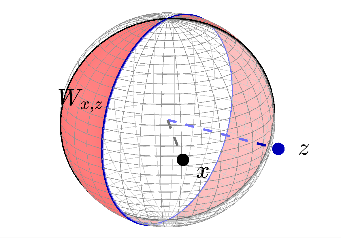
This is the region lying between the two hemispheres with normal vectors $x$ and $z$. We call such a region a spherical wedge, since in three dimensions it has the shape depicted in Figure 1.

When $a\notin W_{x,z}$, we can use the Pythagorean theorem to write

Rearranging gives

where $\tilde{z}=(z-x)/\lVert z-x\rVert_{2}$.

In the complement of this event, we get

and using orthogonality,

Since $z$ gets projected to the hyperplane containing $-x$, it may move further away from $x$. However, we can bound how far away it can move. Because $\langle a,x\rangle$ has the opposite sign as $\langle a,z\rangle$, we have

and so

Substituting this into (2.7), we get the bound

where $\tilde{z}$ is as before.

We can combine (2.6) and (2.8) into a single inequality by writing

Taking expectations, we can remove the role that $\tilde{z}$ plays by bounding this as follows.

We may thus summarize what we have obtained in the following lemma.

Let us next compute what happens for $\mu=\sigma$, the uniform measure on the sphere. It is easy to see that $\mathbb{E}aa^{T}=\frac{1}{n}I_{n}$, so it remains to compute $\mathbb{E}aa^{T}1_{W_{x,z}}(a)$. To do this, we make a convenient choice of coordinates: Let $\theta$ be the angle between $z$ and $x$. We assume that both points lie in the plane spanned by $e_{1}$ and $e_{2}$, the first two basis vectors, and that the angle between $z$ and $x$ is bisected by $e_{1}$, as illustrated in Figure 3.

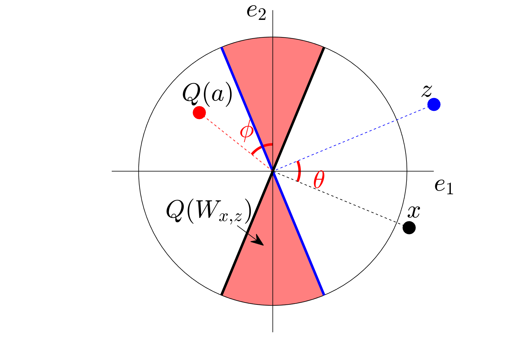
For convenience, denote $M:=\mathbb{E}aa^{T}1_{W_{x,z}}(a)$. Let $Q$ denote the orthogonal projection operator onto the span of $e_{1}$ and $e_{2}$. Then $Q(W_{x,z})$ is the union of two sectors of angle $\theta$, which are respectively bisected by $e_{2}$ and $-e_{2}$. Recall that all coordinate projections of the uniform random vector $a$ are uncorrelated. It is clear that from the symmetry in Figure 3 that they remain uncorrelated even when conditioning on the event that $a\in W_{x,z}$. As such, $M$ is a diagonal matrix.

Let $\phi$ denote the anti-clockwise angle of $Qa$ from $e_{2}$ (see Figure 3). We may write

Note that the magnitude and direction of $Qa$ are independent, and $a\in W_{x,z}$ if either $\phi$ or $\phi-\pi$ lies between $-\theta/2$ and $\theta/2$. We therefore have

By a standard calculation using symmetry, we have $\mathbb{E}\lVert Qa\rVert_{2}^{2}=2/n$. Since $\phi$ is distributed uniformly on the circle, we can compute

As such, we have $M_{11}=(\theta-\sin\theta)/n\pi$, and by a similar calculation, $M_{22}=(\theta+\sin\theta)/n\pi$. Meanwhile, for $i\geq 3$ we have

This implies that

We have now completed proving the following lemma.

In this section, we will show that if we start with an initial estimate that is close enough to the ground truth $x$, then repeatedly applying generalized Kaczmarz projections with respect to the uniform measure $\sigma$ gives linear convergence in expectation. This is exactly the situation we would be in if we were to run randomized Kaczmarz given an unlimited supply of independent sampling vector $a_{1},a_{2},\ldots$ drawn uniformly from the sphere.

We would like to imitate the proof for linear convergence of randomized Kaczmarz for linear systems (Theorem 1.1) given in [18]. We denote by $X_{k}$ the estimate after $k$ steps, using capital letters to emphasize the fact that it is a random variable. If we know that $X_{k}$ takes the value $x_{k}\in\mathbb{R}^{n}$, and the angle $\theta_{k}$ that $z$ makes with $x_{k}$ is smaller than $\pi/8$, then, Lemma 2.2 tells us

where $\alpha_{\sigma}:=1/2-4\sin(\pi/8)/\pi>0$.

The proof for Theorem 1.1 proceeds by unconditioning and iterating a bound similar to (3.1). Unfortunately, our bound depends on $x_{k}$ being in a specific region in $\mathbb{R}^{n}$ and does not hold arbitrarily. Nonetheless, by using some basic concepts from stochastic process theory, we may derive a conditional linear convergence estimate. The details are as follows.

For each $k$, let $\mathcal{F}_{k}$ denote the $\sigma$-algebra generated by $a_{1},a_{2},\ldots,a_{k}$, where $a_{k}$ is the sampling vector used in step $k$. Let $B\subset\mathbb{R}^{n}$ be the region comprising all points making an angle less than or equal to $\pi/8$ with $x$. This is our basin of linear convergence. Let us assume a fixed initial estimate $x_{0}\in B$. Now define a stopping time $\tau$ via

For each $k$, and $x_{k}\in B$, we have

Here, the first inequality follows from the inclusion $\{\tau>{k+1}\}\subset\{\tau>k\}$, the first equality statement from the Markov nature of the process $(X_{k})$, the second equality statement from the fact that $\tau$ is a stopping time, while the second inequality is simply (3.1). Taking expectations with respect to $X_{k}$ then gives

By induction, we therefore obtain

We have thus proven the first part of the following convergence theorem.

We would like to extend the analysis in the previous section to the setting where we only have access to finitely many uniform measurements, i.e. when we are back in the situation of (1.1). When we sample uniformly from the rows of $A$, this can be seen as running the generalized randomized Kaczmarz algorithm using the measure $\mu_{A}=\frac{1}{m}\sum_{i=1}^{m}\delta_{a_{i}}$ as opposed to $\mu=\sigma$.

If we retrace our steps, we will see that the key property of the uniform measure $\sigma$ that we used was that if $W\subset S^{n-1}$ is a wedge²² 2 Recall that a wedge of angle $\theta$ is the region of the sphere between two hemispheres with normal vectors making an angle of $\theta$. of angle $\theta$, then we could make $\lambda_{\max}(\mathbb{E}_{\sigma}aa^{T}1_{W}(a))$ arbitrarily small by taking $\theta$ small enough (see equation (2.9)). We do not actually need such a strong statement. It suffices for there to be an absolute constant $\alpha$ such that

holds for $\theta$ small enough.

Abusing notation, we say that a measurement matrix $A$ is $\textnormal{ACW}(\theta,\alpha)$ if the uniform measure on its rows is $\textnormal{ACW}(\theta,\alpha)$. Plugging in this definition into Lemma 2.1, we immediately get the following statement.

We may now imitate the arguments in the previous section to obtain a guarantee for local linear convergence for the generalized randomized Kaczmarz algorithm using such a measure $\mu$.

Following the theory in the previous section, we see that to prove linear convergence from finitely many uniform measurements, it suffices to show that the measurement matrix $A$ is $\textnormal{ACW}(\theta,\alpha)$ for some $\theta$ and $\alpha$.

For a fixed wedge $W$, we can easily achieve (4.1) by using a standard matrix concentration theorem. By taking a union bound, we can guarantee that it holds over exponentially many wedges with high probability. However, the function $W\mapsto\lambda_{\max}(\mathbb{E}aa^{T}1_{W}(a))$ is not Lipschitz with respect to any natural parametrization of wedges in $S^{n-1}$, so a naive net argument fails. To get around this, we use VC theory, metric entropy, and a chaining theorem from [10].

First, we will use the theory of VC dimension and growth functions to argue that all wedges contain approximately the right fraction of points. This is the content of lemma 5.1. In order to prove this, a fair number of standard definitions and results are required. These are all provided in Appendix A.

References

- [1] Artstein-Avidan, S., Giannopoulos, A., and Milman, V. D. Asymptotic Geometric Analysis, Part I. AMS, 2015.
- [2] Bahmani, S., and Romberg, J. Phase Retrieval Meets Statistical Learning Theory: A Flexible Convex Relaxation. Preprint, available at http://arxiv.org/abs/1610.04210.
- [3] Blumer, A., Ehrenfeucht, A., Haussler, D., and Warmuth, M. K. Learnability and the Vapnik-Chervonenkis dimension. Journal of the ACM 36, 4 (1989), 929–965.
- [4] Candes, E. J., Li, X., and Soltanolkotabi, M. Phase Retrieval via Wirtinger Flow: Theory and Algorithms. IEEE Transactions on Information Theory 61, 4 (2015), 1985–2007.
- [5] Candes, E. J., Strohmer, T., and Voroninski, V. PhaseLift: Exact and stable signal recovery from magnitude measurements via convex programming. Communications on Pure and Applied Mathematics 66, 8 (2013), 1241–1274.
- [6] Chen, Y., and Candes, E. Solving random quadratic systems of equations is nearly as easy as solving linear systems. In Advances in Neural Information Processing Systems 28. 2015, pp. 739–747.
- [7] Chi, Y., and Lu, Y. M. Kaczmarz Method for Solving Quadratic Equations. IEEE Signal Processing Letters 23, 9 (2016), 1183–1187.
- [8] Davis, C., and Kahan, W. M. The rotation of eigenvectors by a perturbation. III. SIAM Journal on Numerical Analysis 7, 1 (1970), 1–46.
- [9] Davis, D., Drusvyatskiy, D., and Paquette, C. The nonsmooth landscape of phase retrieval.
- [10] Dirksen, S. Tail bounds via generic chaining. Electronic Journal of Probability 20 (2015), 1–29.
- [11] Duchi, J. C., and Ruan, F. Solving (most) of a set of quadratic equalities: Composite optimization for robust phase retrieval. Preprint, available at http://arxiv.org/abs/1705.02356.
- [12] Eldar, Y. C., and Mendelson, S. Phase retrieval: Stability and recovery guarantees. Applied and Computational Harmonic Analysis 36, 3 (2014), 473–494.
- [13] Fienup, J. R. Phase retrieval algorithms: a comparison. Appl. Opt. 21, 15 (1982), 2758.
- [14] Goldstein, T., and Studer, C. PhaseMax: Convex Phase Retrieval via Basis Pursuit. Preprint, available at http://arxiv.org/abs/1610.07531.
- [15] Hand, P., and Voroninski, V. An Elementary Proof of Convex Phase Retrieval in the Natural Parameter Space via the Linear Program PhaseMax. Preprint, available at http://arxiv.org/abs/1611.03935.
- [16] Jeong, H., and Güntürk, C. S. Convergence of the randomized Kaczmarz method for phase retrieval. Preprint, available at http://arxiv.org/abs/1706.10291.
- [17] Mohri, M., Rostamizadeh, A., and Talwalkar, A. Foundations of Machine Learning. MIT press, 2012.
- [18] Strohmer, T., and Vershynin, R. A randomized kaczmarz algorithm with exponential convergence. Journal of Fourier Analysis and Applications 15, 2 (2009), 262–278.
- [19] Sun, J., Qu, Q., and Wright, J. A Geometric Analysis of Phase Retrieval. Foundations of Computational Mathematics (2017).
- [20] Talagrand, M. The Generic Chaining: Upper and Lower Bounds of Stochastic Processes. Springer Monographs in Mathematics. Springer Berlin Heidelberg, 2005.
- [21] Vapnik, V. N., and Chervonenkis, A. Y. On the Uniform Convergence of Relative Frequencies of Events to Their Probabilities. Theory of Probability & Its Applications 16, 2 (Jan 1971), 264–280.
- [22] Vershynin, R. High-Dimensional Probability. Book draft, available at https://www.math.uci.edu/~rvershyn/papers/HDP-book/HDP-book.html.
- [23] Vershynin, R. Introduction to the non-asymptotic analysis of random matrices. In Compressed Sensing, Y. C. Eldar and G. Kutyniok, Eds. Cambridge University Press, Cambridge, 2011, pp. 210–268.
- [24] Wang, G., Giannakis, G. B., and Eldar, Y. C. Solving Systems of Random Quadratic Equations via Truncated Amplitude Flow. IEEE Transactions on Signal Processing 65, 8 (May 2016), 1961–1974.
- [25] Wei, K. Solving systems of phaseless equations via Kaczmarz methods: a proof of concept study. Inverse Problems 31, 12 (Dec 2015), 125008.
- [26] Zhang, H., and Liang, Y. Reshaped wirtinger flow for solving quadratic system of equations. In Advances in Neural Information Processing Systems 29. 2016, pp. 2622–2630.
Appendix A Growth functions and VC dimension
In this section, we define growth functions and VC dimension. We also state some standard results on these topics that we require for our proofs in Section 5. We refer the interested reader to [17] for a more in-depth exposition on these topics.
Let be a set and be a family of subsets of . For a given set , we slightly abuse notation and identify it with its indicator function .
The growth function of is defined via
Meanwhile, the VC dimension of is defined to be the largest integer for which . These two concepts are fundamental to statistical learning theory. The key connection between them is given by the Sauer-Shelah lemma.
Lemma A.1 (Sauer-Shelah, Corollary 3.3 in [17]).
Let be a collection of subsets of VC dimension . Then for all , have
The reason why we are interested in the growth function of a family of subsets is because we have the following guarantee for the uniform convergence for the empirical measures of sets belonging to .
Proposition A.2 (Uniform deviation, Theorem 2 in [21]).
Let be a family of subsets of a set . Let be a probability measure on , and let be the empirical measure obtained from independent copies of a random variable with distribution . For every such that , the following deviation inequality holds: