CALT-TH-2017-033
Quasi-Single Field Inflation in the non-perturbative regime
Abstract
In quasi-single field inflation there are massive fields that interact with the inflaton field. If these other fields are not much heavier than the Hubble constant during inflation () these interactions can lead to important consequences for the cosmological energy density perturbations. The simplest model of this type has a real scalar inflaton field that interacts with another real scalar (with mass ). In this model there is a mixing term of the form , where is the Goldstone fluctuation that is associated with the breaking of time translation invariance by the time evolution of the inflaton field during the inflationary era. In this paper we study this model in the region and or less. For a large part of the parameter space in this region standard perturbative methods are not applicable. Using numerical and analytic methods we study how large has to be for the large effective field theory approach to be applicable.
I Introduction
There is very strong evidence that the universe was once in a radiation dominated era followed by a matter dominated era. Today the universe is dominated by vacuum energy density and we are entering an inflationary era where the scale factor , with near the Hubble constant today. It is widely believed that at very early times there was another inflationary era where the energy density was dominated by false vacuum energy giving rise to a Robertson Walker scale factor with time dependence , where is the Hubble constant during that inflationary era [1, 2]. After more than about 60 e-folds, this inflationary era ends and the universe reheats to a radiation dominated (Robertson Walker) Universe. If this is the case then the horizon and flatness problems [2] can be solved and in addition there is an attractive mechanism based on quantum fluctuations for generating density perturbations with wavelengths that were once outside the horizon [3] (see Ref. [4] for a review of inflation). It has been argued that it requires tuning to enter the inflationary era [5] (see however [6]) and furthermore that there are issues with its predictability [7] (see also [8] for a recent discussion of these issues). Nevertheless, because of the simplicity of the dynamics of the inflationary universe paradigm and the ability within it to do explicit calculations of the properties of the cosmological energy density perturbations [3] and primordial gravitational waves [9], it seems worth studying particular inflationary models in some detail.
The simplest inflationary model is standard slow roll inflation with only a single real scalar field, the inflaton . It is conventional to work in a gauge where fluctuations in the inflaton field about the classical slow roll solution vanish. Then using the Stckelberg trick the curvature fluctuations that are constant outside the horizon and become the density perturbations when they reenter the horizon (in the radiation and matter dominated eras) arise from quantum correlations in the Goldstone mode calculated during the de-Sitter inflationary era11 1 The effective field theory formulation for inflation [10] provides an elegant method to compute correlations of in a model independent fashion.. In this model non gaussianities in cosmological density correlations arise because of connected higher point correlations of , but they are very small [11].
Larger non-gaussianities can be achieved if there are other fields with masses around or less than the inflationary Hubble constant22 2 There are other ways to have large non-gaussianities. For example, DBI inflation [12]. For an early example of another type, see [13]., that couple to (see Ref. [14] for a review). In quasi-single field inflation these extra fields do not directly influence the classical evolution of the inflaton field but impact the cosmological density perturbations since they couple to the inflaton as “virtual particles” and hence affect the the correlations of [15]. To simplify matters we will assume an approximate shift symmetry on the inflaton field, (where is a constant) that is only broken by the potential, , for . Furthermore, we assume an unbroken discrete symmetry, . The simplest quasi-single field model introduced by Chen and Wang [14] has a single additional (beyond the inflaton) real scalar field . The Lagrange density in this model contains an unusual kinetic mixing of the form .
This model has been extensively studied in the perturbative region33 3 By perturbation theory we mean a series expansion in . where [15, 16, 17, 18, 19, 20, 24, 21, 22, 23]. In the non-perturbative region where , an elegant effective field theory formulation has been derived by Baumann and Green [24], and by Gwyn, Palma, Sakellariadou, and Sypsas [25]. The curvature perturbation power spectrum and a contribution to its bispectrum have been calculated using this formulation. It has been studied numericaly in [26] for other regions of the parameter space.
Throughout this paper we treat as a constant independent of time. There has been a study of the case where changes suddenly with time, becoming large momentarily [27].
In this paper we focus on the region of parameter space where and or less (recall is the mass term for ). In this region, non-gaussianities have an interesting oscillatory behavior [19]. We use numerical non-perturbative methods similar to those developed in [26] and the effective field theory for large to study the model in this region of parameter space. We study how large must be for the effective field theory method to be quantitatively correct. In addition we derive the , plot for the model with inflaton potential and derive the limit on and the potential parameter from Planck limits on non-gaussianity.
In section II we discuss the Lagrange density of the model we use in detail. Section III reviews quantization of the free part of the Lagrange density in flat space-time. Even this theory is non-trivial because of the unusual Lorentz non-invariant kinetic mixing between the Goldstone field and the excitations of the massive scalar . The massless mode has an unusual energy momentum relation that, for momentum in the range , has a non-relativistic flavor, [24]. The other mode is heavy with a mass . The fact that this mode’s mass does not go to zero as is what regularizes the divergences that occur at when one treats perturbatively.
Quantization of the free field theory in de-Sitter space-time is discussed in section IV. In de-Sitter space-time a mode’s physical momentum evolves with time. At early times modes have wavelengths much less than the horizon but at later times the wavelengths get red-shifted outside the horizon. The mode functions are calculated non-perturbatively by numerically solving the differential equations they satisfy in the region of parameter space, and or less. Quantum fluctuations in the field fall off rapidly for wavelengths outside the horizon and it is the quantum fluctuations in the field that determine the curvature and density fluctuations just as in standard slow roll single field inflation. Nevertheless, these quantum fluctuations are influenced by ’s couplings to .
In section IV we analyze (in the non-perturbative regime) the curvature perturbation power spectrum in this model focusing on the transition between the perturbative regime and the regime where the effective theory applies. Section V derives the plot in this theory for the simple inflaton potential .
Non-gaussianities are discussed in Sec VI. We calculate the bispectrum in the the equilateral and squeezed configurations in the non-perturbative region numerically. In the large region we show that the numerical results agree with the results from the effective theory. We derive the constraints on and the potential parameter from Planck limits on non-gaussianity.
In section VII we review the derivation of the effective field theory for large and the derivation of the power spectrum using it. We then compute the bispectrum in this effective field theory including a contribution from the potential for that was not previously presented in the literature.
Our conclusions are summarized in Sec. VIII.
II The Model
The simplest quasi-single field inflation model has a real scalar inflaton field that interacts with another real scalar field . We impose a symmetry and an approximate shift symmetry , where is a constant. The shift symmetry is only broken by the inflaton potential . The Lagrangian we use has the form
| (1) |
where
| (2) |
Interactions between the inflaton and the massive field first occur at dimension 5 and if we neglect operators with dimension higher than this the interaction Lagrangian is
| (3) |
One natural choice for the mass scale is the Planck mass. This higher dimensional operator would then arise from the transition from the theory of quantum gravity to a quantum field theory. In this case the non-gaussianities are very small. However, another possibility is that there is physics at a scale that is large compared to the Hubble constant during inflation but well below the Planck scale. Integrating out this physics can give rise to such an operator.
We work in a gauge where the inflaton field is only a function of time, and take the background metric to have the form, , with the scale factor . The Goldstone boson associated with the time translation invariance breaking by the classical evolution is denoted by . The curvature perturbation is proportional to this field, . We expand about a background classical value and assume that the background solution is independent of time. This assumption is consistent with the dynamical equations of evolution for the fields provided we neglect second time derivatives of . With those assumptions and satisfy,
| (4) |
and
| (5) |
The dynamics for the fluctuations and are controlled by the Lagrange density,
| (6) |
where the free part of the Lagrange density for the fields and is,
| (7) |
where . Throughout this paper we assume that the mass parameter for the additional scalar is of order the Hubble constant during inflation or smaller.
The interaction part of the Lagrange density is
| (8) |
It is convenient to introduce a rescaled that has a properly normalized kinetic term,
| (9) |
where,
| (10) |
In terms of these rescaled fields the gravitational curvature perturbation becomes,
| (11) |
The free and interacting Lagrange densities, after introducing a redefined scale , are
| (12) |
and
| (13) |
In eq. (12) we have introduced
| (14) |
and in eq. (13) only explicitly kept those terms that play a role in the calculations performed in this paper. In the following sections we will drop the tilde on the Goldstone field to simplify the notation. Moreover, we adopt sign conventions for and so that and are positive.
As mentioned in the introduction the purpose of this paper is to study this model in the region of parameter space where and or smaller. Some of this region, i.e. where is small or very large have been previously studied. We will compare with those results to find out how small and how large has to be for the approximate methods used in those regions to be accurate.
First let’s imagine that =0. This can always be arranged by tuning the linear term in the potential to cancel the linear term in from the interaction term. Then . The measured power spectrum for the curvature perturbations implies that is very large so even for small one can achieve large values for .
Next we allow a non zero but simplify the potential so it contains no terms with more than two powers of , explicitly . In this case can be written as,
| (15) |
Therefore, without tuning the tadpole in to cancel , it is not possible to have the mass parameter of order the Hubble constant (or smaller) and large. Nonetheless it seems worth studying this region of parameter space since there are some novel features that arise there.
Naive dimensional analysis suggests that higher dimension operators that couple derivatives of to a single are smaller than the dimension 5 operator we kept provided . The higher powers of will be small if in addition . Since the measured amplitude of the density perturbations implies that is quite small the ratio can be large in the region of parameter space where the operator expansion in powers of is justified. Indeed, comparing the calculated power spectrum at large given in (37) with it’s measured value, the upper limit for for power counting in the expansion to be valid is . Of course, this is just a naturalness constraint and can be violated without the model being inconsistent.
III Free Field Theory in Flat Space-time
In this section we review, for pedagogical reasons, quantization in flat space-time of the free field theory with Lagrange density in eq. (12). The results presented here have, by in large, been noted previously in [24, 25].
Dropping the tildes and setting the Lagrange density in eq. (12) becomes,
| (16) |
This corresponds to normal kinetic terms for two real scalar fields but with an unusual Lorentz non-invariant kinetic mixing. The Lagrange density has the shift symmetry for the Goldstone field .
The classical equations of motion for the fields and are,
| (17) |
and
| (18) |
Quantization proceeds by expanding the fields in modes,
| (19) |
and
| (20) |
The annihilation operators and creation operators satisfy the usual commutation relations44 4 More explicitly the non-zero commutators are: and . The time dependence of the mode functions and are determined by solving the classical equations of motion and their normalization is fixed by the canonical commutation relations of the fields with their canonical momenta. A difference from the usual case where there is no Lorentz non-invariant mixing is that the canonical momentum for the field is not but rather . So and don’t commute at equal time but rather satisfy .
The time dependence of the modes has the usual exponential form , . The dispersion relations for the energies is determined by solving the classical equations of motion. This yields,
| (21) |
which is a massless mode that we label by (1) corresponding to the minus sign and a massive mode that we label by (2) corresponding to the plus sign. The mass of mode (2) is . Because this mode remains massive even when there will be no divergences in our calculations in de-Sitter space.
We now focus on the large mixing region of parameter space, . As discussed in the literature [24] the dispersion relations of the two modes can be written as
| (22) |
The mode is massless but for much larger than the energy grows not linearly with but rather quadratically (like a non relativistic particle). The other mode is massive with mass . For very small momentum, , the massive scalar only contains the massive mode, i.e., as . On the other hand the Goldstone field contains equal amounts of the and modes.
The infrared, , behavior of the mode function changes in the special case that . Then integrating-by-parts, the kinetic mixing term in Eq. (16) can be recast as , and so it is clear that there is also a shift symmetry in . For the scalar field also contains equal amounts of the two modes.
Since for large the second mode is heavy it is appropriate for the physics at low momentum to integrate it out from the theory and write an effective Lagrange density in terms of a single massless field. For the light mode a time derivative gives factors of and (for ) at very large the field contains only a small amount of that massless mode. Hence eq.(18) imples that,
| (23) |
Putting this into the Lagrange density in eq. (16) and dropping terms suppressed by powers of (recall a time derivative on is suppressed by ) yields the effective Lagrange density for the massless mode,
| (24) |
which yields the dispersion relation for the massless mode given in eq. (22).
In the next section we perform the quantization in curved de-Sitter space-time (with Hubble constant ). Then the physics of the massless mode should be similar to that in flat space-time when the momentum and energy for that mode are large compared to i.e., and . In the flat space-time large discussion we assumed . The energy condition implies must also satisfy in order for our de-Sitter space-time computations to resemble the flat space-time large case discussed in this subsection.
IV Free Field Theory in de-Sitter Space time
Introducing conformal time, , and including the measure factor in the Lagrange density so that the action is equal to we have
| (25) |
As in flat space we expand the quantum fields in terms of creation and annihilation operators. Introducing we write,
| (26) |
and
| (27) |
The mode functions obey the classical equations of motion,
| (28) |
and
| (29) |
where a “ ′ ” represents an derivative.
IV.1 Numerical results
In the mode expansion for for the fields and , is the magnitude of the comoving wavevector. The physical wavevector has magnitude . Hence the condition that a mode have wavelength well within the de-Sitter horizon is which is equivalent to . At fixed as time evolves a mode goes from physical wavelength well within the horizon to outside the horizon.
In the region well within the horizon, and , the differential equations (28) and (29) simplify to
Here we suppressed the superscripts that label mode type. The leading behavior of the mode functions is
| (31) |
and so it is convenient to represent the general solution in the region deeply inside the horizon as
| (32) |
and are functions of with . Substituting and back into (28) and (29) and keeping only the leading order terms in we find
| (33) |
which gives
| (34) |
Therefore, in this region the canonically normalized form of and can be written as
| (35) |
where the factor is determined by the canonical commutation relations.
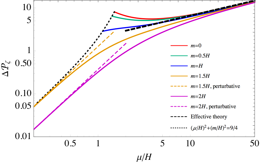
Eq. (35) is used to determine the initial conditions , and , at a value of that is large in magnitude. The differential equations in (28) and (29) can then be solved numerically and used to determine the power spectrum for the curvature perturbation in this model.
The correction to the power spectrum is defined by, , where
| (36) |
is the power spectrum of the curvature perturbation in usual slow roll single field inflation. is shown in Fig. 1. In the region of goes like which agrees with the perturbative calculation [15]. In the region where is larger than about the power spectrum grows as and can be approximated by,
| (37) |
where
| (38) |
Corrections to eqs. (37) and (38) become negligible as . The power spectrum in the large limit was calculated using the large effective field theory in [25]. For completeness we briefly review that calculation in Sec. VII.
As shown in Ref. [15], the perturbative result diverges in the limit of . From the red curve shown in Fig. 1 we can see that the curvature perturbation is well defined at . Perturbation theory can be very misleading at modest values of and values of not very much larger than unity. For example for and it gives a value for (in the units used for Fig. 1) equal to 310 while our numerical result is 6.2.
For the curvature perturbations one calculates the power spectrum of the field as . However the power spectra for the fields can be calculated at any . For the power spectrum for the field falls off rapidly as falls below unity. The numerical results of the power spectrum of the field in units of as a function of for a few values of and are shown in Fig. 2. One can see that all the curves decrease with and become small as falls below unity.
In the usual single field inflation model goes to unity in units of as . In this model of quasi-single field inflation, as shown in Fig. 2 for the , case the asymptotic value of is much larger than unity. This is due to the change in the dispersion relation of the field and can be understood using the large effective theory. From Fig. 2 we see that the asymptotic value of for the case is also much larger than 1.
IV.2 Qualitative analysis
We can understand qualitatively the shape of the mode functions analytically. In the region well outside the horizon, , eqs. (28) and (29) can be simplified to
| (39) |
which is invariant under the transformation
| (40) |
Therefore, the general form of the solution can be written as
| (41) |
Putting this back into the differential equations gives equations for the power and the coefficients and
| (42) |
To have nontrivial solutions for and requires
| (43) |
There are four solutions to this equation
| (44) |
For the region of parameter space we focus on, are complex, which can have observational consequences for the non-gaussianities [19].
For large values of the infrared behavior of the mode functions and match directly onto the solutions in eq. (44). This is shown in Fig. 3 using and . The mode is constant outside the horizon. The behavior vanishes outside the horizon and can be thought of as a subdominant contribution to the massless mode. The solutions correspond to the mode functions for a free scalar field with mass equal to . They play an important role in the calculation of non-gaussianities. For and the behavior of this mode is shown by the blue dot-dashed curves in Fig. 3. One can see that it oscillates logarithmically with frequency , and decreases with a power of for small . To get the curves shown in Fig. 3 we solve the differential equations (28) and (29) with the initial conditions (35). The mode shown in the left panel of Fig. 3 eventually goes to a constant as gets smaller. Similarly, the absolute value of the mode eventually goes like for very small .
In this paragraph we focus on the solution. Putting back Eq. (42) we find that . Since there is no shift symmetry in the field it should not contain the massless mode in the far infrared. We can get the leading behavior of the mode function outside the horizon by putting back into the exact differential equation (28). This gives the first order inhomogeneous differential equation
| (45) |
with general solution
| (46) |
This behavior is shown by the red dashed curves in Fig. 3.
IV.3 The large region
In this subsection we focus on some properties of the solutions for the mode functions that only apply for very large . We find that the curvature perturbation goes to a constant when instead of the usual condition that it be outside the horizon, i.e., . This is illustrated in Fig. 4 which shows the numerical results for the power spectrum of as a function of .
Examining eq. (29), in the region it is clear that the last term on the left hand side is the largest. Neglecting the other terms the solution in this region satisfies
| (47) |
which implies that is constant and is proportional to , as in eq. (46).
In the region one can show that the differential equations for the mode functions are solved approximately by
| (48) |
The physical wavevector of a mode with comoving wavevector is
| (49) |
Therefore the change of the phase of these solutions within a small time period can be written as
| (50) |
where has been used. This agrees with the dispersion relation in flat space given in eq. (22) for the massless mode. From Fig. 4, one can see that it is in this region the solution for starts to deviate from the standard slow roll solution, which corresponds to in the model we are studying. This is because in this region the solutions in de-Sitter space should resemble those in flat space and the light mode has a flat space dispersion relation which is quite different from a single massless field with dispersion relation .
Putting the solution we have found back into the differential equations (28) and (29), one can see that the terms
| (51) |
are suppressed, which means that the terms
| (52) |
in the Lagrange density (25) can be neglected. After neglecting these two terms, there are no terms in (25) that contain time derivatives of . This indicates that has become a Lagrange multiplier and can be replaced in the Lagrange density using its classical equation of motion to express it in terms of . This amounts to summing the tree graphs that contain virtual propogators and is the origin of the effective theory approach developed in Refs. [24] and [25] for the behavior of in this region. We will briefly review the basic setup for this effective field theory and use it to calculate the two- and three-point functions of the curvature perturbation in the large limit in Sec. VII.
V Impact on observables
The dimensionless power spectrum is defined as [28]
| (53) |
where is a function of the and . is shown in Fig. 1 as a function of for fixed values of . Throughout this section we neglect the impact of the time dependence of on the value of since, as was discussed in section II, it is suppressed by a power of .
In terms of the slow-roll parameter
| (54) |
can be written as
| (55) |
The tilt of the power spectrum is defined as
| (56) |
and can be written as
| (57) |
where is the number of e-folds between when the modes of interest exit the horizon and inflation ends. From Eq. (53) we have
| (58) | |||||
where the standard results of slow-roll inflation have been used [4], and is the other slow-roll parameter defined as . and are defined as
| (59) |
Up to leading order in the slow-roll parameters we have that,
| (60) |
Therefore at leading order in slow roll parameters
| (61) |
Another important observable is the tensor-scalar ratio. Since the gravitational wave production is only related to the structure of the de-Sitter metric, the dimensionless tensor spectrum can still be written as
| (62) |
Then the tensor-scalar ratio can be written
| (63) |
V.1 inflation

Here we use the model where the inflaton potential as an example to discuss the effect of large on the observables. In this simple model, we have
| (64) |
and
| (65) |
where is the number of e-folds between when CMB scale leaves the horizon and when slow roll inflation ends.
The plot for this model is shown in Fig. 5. The dotted regions are for from 0 to and from to with . On these curves as increases decreases, so the uppermost point of the curves corresponds to standard slow roll inflation. The constraints on the parameter space for and 60 are also shown in Fig. 6 where the regions below the curves are excluded. Clearly larger values of improve the agreement of the model’s predictions with the measured value of and the bound on .
VI Non-Gaussianities
In this section we calculate the dependence of the inflaton three-point function as a function of and . The small behavior of the bispectrum was first studied in [15]. The effective field theory for large was used to compute the contribution from the interaction to the bispectrum [24, 25]. Here we use the numerical mode functions to extend the analysis to other values of .
The curvature perturbation bispectrum is defined by
| (66) |
and we can define analogously. They can be computed using the in-in formalism [31] using the interaction Lagrangian in eq. (13).
In this section we focus mostly on the term (where ) which, for , typically dominates over the contribution from the term. We express the contribution to the bispectrum in terms of the mode functions discussed earlier. Evaluating the correlator in the far future , we find
| (67) |
Equation (67) is true for all values of , however we are mostly interested in its behavior in the so-called equilateral and squeezed limits. In the equilateral limit, the external momenta all have equal magnitude . In this case, the integral’s dependence on can be factored out of the integral by rescaling the integration variable from to :55 5 By, , we mean evaluated in the equilateral configuration where the three wavevectors have the same magnitude .
| (68) |
We can compute this integral numerically using the numeric mode functions, but there are a couple of subtleties in its evaluation that need to be addressed. The integrand in (68) is highly oscillatory at large . For and values of order one or larger, the magnitude of these oscillations does not decay quickly and it becomes difficult to perform the numerical integrations by brute force. We can alleviate this problem by Wick rotating the integral, thereby transforming the rapid oscillations into exponential decay.
Before Wick rotating it is convenient to factor out the oscillatory behavior from the mode functions. The large limit given in eq. (32) suggests that we should extract the oscillatory behavior by factorizing the mode functions as and . Plugging this factorization into gives
| (69) | ||||
| (70) |
In the second line we used Cauchy’s theorem to rotate the region of integration from the real to the imaginary axis and changed the integration variable from to .
The numerical solutions found previously for and are functions of the real variable and cannot be integrated along the imaginary axis. However, we can analytically continue them to the imaginary axis by Wick rotating the original mode equations (28) and (29) (see [26]). After factoring out the oscillatory behavior and changing variables to , we find that the analytically continued functions and obey
| (71) | ||||
| (72) |
where a prime denotes a derivative with respect to and we have dropped the superscripts for simplicity. The solutions should asymptote at large to66 6 If we hadn’t first extracted the oscillatory factor, an exponentially suppressed factor would have appeared in (73) that would have made the boundary conditions too small to solve (71) numerically.
| (73) | ||||
| (74) |
These solutions and their derivatives with respect to give the initial conditions for numerical integration of the differential equations for and . Note that and contain an overall factor of . Moreover, and have the same -dependent normalization. This implies that is -independent.
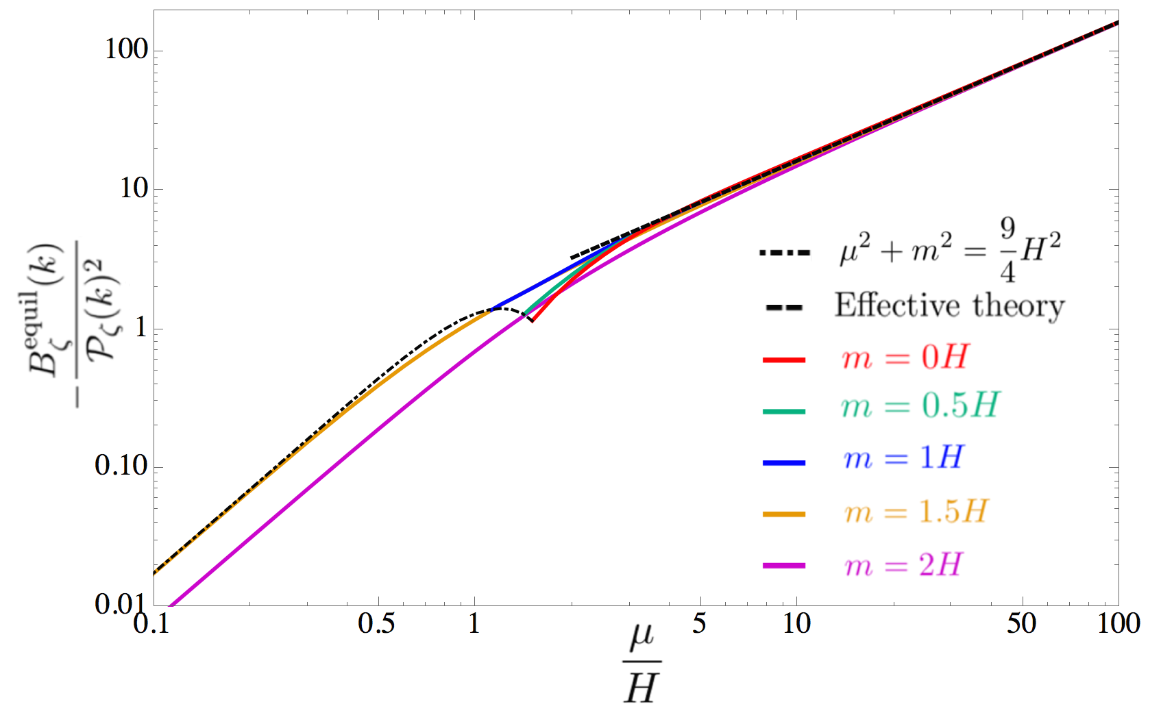
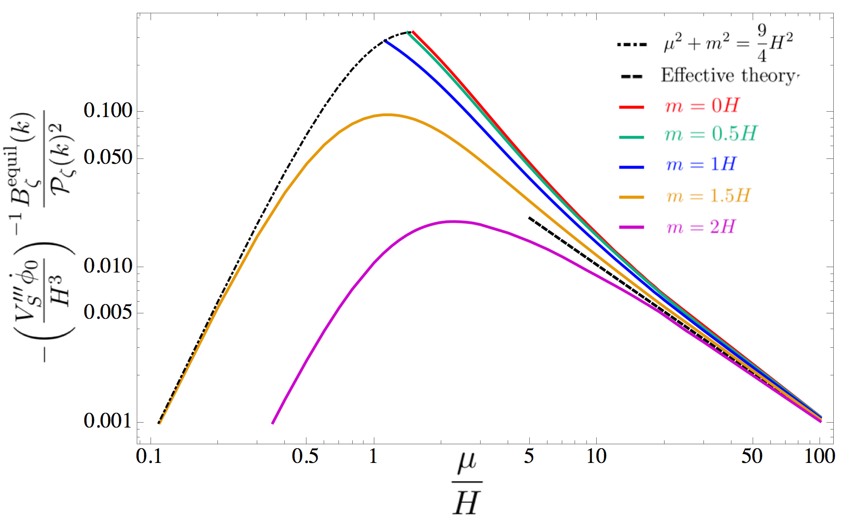
In figures 8 and 8, we plot the contributions to the scaled equilateral three-point functions due to the and interaction terms respectively77 7 For brevity we have not described in any detail the calculation of the contribution due to the term in this section.. Moreover, we have superimposed a dotted line which corresponds to the prediction of the effective field theory appropriate for large (which will be discussed in detail in section VII). Of course, the numerical results converge to the effective field theory results in the large limit. However, the effective field theory is only a good approximation of these non-gaussianities for . This further suggests that there is a substantial portion of the parameter space in that is described neither by the large effective theory description nor the small perturbative description.
The Planck collaboration has derived constraints on the magnitude of the bispectrum of the curvature perturbations using various models/templates for its dependence on the wavevectors [30]. These are usually expressed in terms of the quantity . Although the model we are discussing is different from the equilateral model/template used to derive the constraint by the Planck collaboration in Ref. [30], we use this constraint to estimate a bound on . Furthermore we estimate using just the equilateral configuration where the three wavevectors have the same magnitude taking,
| (75) |
To determine upper bounds for we assume that each interaction and is separately constrained by and thus ignore any possible tuning between the two terms that may make these bounds weaker. Figure 9 shows the upper bounds for a variety of masses, as well as the upper bound predicted in the large effective theory.


The squeezed limit of (67) occurs when . In this limit, define the ratio , where , and introduce the notation for . We again rescale the integration variable to to find
| (76) | ||||
| (79) | ||||
| (80) |
We can analyze the leading behavior of (76) in by replacing with the first few terms of its power series expansion (see section IV.2) :
| (81) | ||||
| (82) |
where , , and
| (83) | ||||
| (84) | ||||
| (85) |
We can compute , , and by fitting the numerical mode functions to their power series expansions at small and extracting , from the fits. The integrals in (83) can be computed using the same Wick rotation technique used to compute . Then, rearranging (81) gives
| (86) | ||||
We plot in figure 10. The sine term is usually smaller and so we have not displayed it in a figure. Equation (86) shows that the squeezed limit of the three-point function oscillates logarithmically as a function of . This behavior is illustrated in figure 11. Note that that the dependence of on has an important effect on the oscillations. This impacts the two point function of biased objects, see for example [32].
The oscillatory terms in eq. (86) are enhanced by a factor of , but are suppressed in the large limit.
VII Calculating non-gaussianity in the effective theory
VII.1 Brief review of the effective theory for large
In this subsection we begin with a brief review the effective theory approach to the case when is large. In terms of and the Lagrange density is
As discussed in Sec. III, in flat space-time with large mixing there is a very massive mode and a massless mode. When and , one may integrate out the heavy mode to get an effective theory just involving which can be used to calculate curvature perturbations. As discussed in Sec. IV, for that purpose the and terms in eq. (VII.1) can be neglected. Since we assume or smaller can also be neglected in eq. (VII.1). With these approximations the equation of motion for becomes
| (88) |
Up the second order in , the solution for is
| (89) |
Putting this solution back into eq. (VII.1), the quadratic and cubic terms of the effective Lagrangian of can be written as
| (90) |
and
| (91) |
Quantizing the free field part of this effective theory we write for the field operator,
| (92) |
The mode function satisfies the classical equation of motion,
| (93) |
which can be solved analytically for the mode function . The normalization of is determined by the canonical commutation relations. This yields,
| (94) |
The power spectrum of the curvature perturbation is
| (95) |
The plot of as a function of was shown in Fig. 1. The result from the effective theory is shown by the black dashed line. One can see that for the result from the effective theory agrees with the numerical result.
VII.2 Non-Gaussianity of equilateral configuration
The three-point function of the curvature perturbation is defined in (66). Following standard steps and using the explicit expression of in (94) for the equilateral configuration (), we have
| (96) |
where
| (97) |
As previously discussed we take
| (98) | |||||
The factor can be calculated in terms of the density perturbation and using (53). Using the measured value of we have that
| (99) |
In addition, using the Planck data, the constraint on is estimated to be88 8 Here we have neglected the term. It is of course possible that there are cancelations between the contribution proportional to and that proportional to which would relax the bound on .
| (100) |
VII.3 Non-gaussianity of squeezed configuration
For the squeezed configuration we consider . Taking the contribution from the term in the interaction Lagrange density we have
| (101) |
where
| (102) | ||||
| (103) |
Note that and oscillate rapidly when . Therefore, the integral is mainly supported in the region , which means . Around we have
| (104) |
which implies that
| (105) |
For , and go like and we have that in the squeezed limit . Even though this contribution is enhanced by a power of , it is still suppressed compared to what local non-gaussianity would give which is proportional to . This behavior in the squeezed limit is also seen in equilateral non-Gaussianity.
For the contribution proportional to we find
| (106) |
where in this case
| (107) |
Therefore, the interaction also gives a contribution to .
VIII Concluding Remarks
We studied a simple quasi-single field inflation model where the inflaton couples to another scalar field . The model contains an unusual mixing term between the inflaton and the new scalar characterized by a dimensionful parameter . It has been extensively studied in the literature using perturbation theory in the region where the parameter is small and using an effective field theory approach in the region of large . It has also been studied using numerical methods in other regions of parameter space. When the mass parameter of the additional scalar field is zero perturbation theory diverges.
We numerically calculated the power spectrum and the bispectrum of the curvature perturbations when and the mass satisfy with or smaller. In much of this region, perturbation theory and the effective field theory approach are not applicable. We found that typically the effective field theory approach is valid for . The numerical approach is non-perturbative in and there are no divergences at . This occurs because the heavy mode has mass which does not vanish as .
In the case where the inflaton potential is , we derived constraints on the parameters and from and for and . Larger values of make this inflaton potential more compatible with the data.
We computed the contributions from the and the interactions to the equilateral limit of the bispectrum of the curvature perturbations numerically and compared it with the results from the effective theory. Using these results and the Planck bounds on we derived upper bounds on and .
We also analyzed the squeezed limit of the bispectrum, showing that in this model it is much smaller than for local non-gaussianity. The contribution to the squeezed bispectrum proportional to exhibits interesting oscillatory behavior as a function of the ratio of the small momenta to the larger one.99 9 This oscillatory behavior was previously noted using perturbation theory for the contribution of the interaction to the bispectrum and trispectrum [19]. We noted that the oscillation wavelength has dependence that is not evident in perturbation theory. This behavior could potentially be observed in future experiments.
For small and , there are potentially interesting observational consequences of the behavior of the four point function on the wavevectors that characterize its shape. We will present results on this in a further publication.
Acknowledgements.
HA would like to thank Asimina Arvanitaki, Cliff Burgess and Yi Wang for useful comments and discussions. This work was supported by the DOE Grant DE-SC0011632. We are also grateful for the support provided by the Walter Burke Institute for Theoretical Physics.References
- [1] A. A. Starobinsky, JETP Lett. 30, 682 (1979); Phys. Lett. B. 91, 99 (1980); D. Kaznas, Atrophys. J. 241, L59 (1980); K. Sato, Mon. Not. Roy. Astron. Soc. 195 467 (1981).
- [2] A. Guth, Phys. Rev. D23, 347 (1981); A. D. Linde, Phys. Lett. B 108, 389 (1982); 114, 431 (1982); A. Albrecht and P. Steinhardt, Phys. Rev. Lett. 48, 1220 (1982).
- [3] S. V. Mukanov and G. V. Chibisov, Sov. Phys. JETP Lett. 33, 532 (1981); S. Hawking, Phys. Lett. B115, 295 (1982); A. A. Starobinsky, Phys. Lett. B 117, 175 (1982); A. Guth and S.-Y. Pi, Phys. Rev. Lett 49, 1110 (1982); J. M. Bardeen, P. Steinhardt and M. S. Turner, Phys. Rev. D28, 679 (1983).
- [4] D. Baumann, doi:10.1142/9789814327183-0010 arXiv:0907.5424 [hep-th].
- [5] R. Penrose, Annals N.Y. Acad. Sci., 571, 249, (1989); G. Gibbons and N. Turok, Phys. Rev. D77, 063516 (2008).
- [6] M. Bastero-Gil, A. Berera, R. Brandenberger, I. G. Moss, R. O. Ramos and J. G. Rosa, arXiv:1612.04726 [astro-ph.CO].
- [7] P. J. Steinhardt, in The Very Early Universe, edited by G. Gibbons, H.S., and S. Siklos, Cambridge University Press, pp.251-266 (1983); A. Vilenkin, Phys. Rev. D27, 2848 (1983); A. H. Guth, Phys, Rept. 333, 555 (2000).
- [8] A. Ijjas, P. J. Steinhardt and A. Loeb, Phys. Lett. B 723, 261 (2013), doi:10.1016/j.physletb.2013.05.023, [arXiv:1304.2785 [astro-ph.CO]]; Phys. Lett. B 736, 142 (2014) doi:10.1016/j.physletb.2014.07.012 [arXiv:1402.6980 [astro-ph.CO]].
- [9] L. P. Grishchuk, Sov. Phys. JETP 40, 409 (1974); A. A. Starobinsky, Sov. Phys. JETP Lett. 30, 682 (1979); V.A. Rubakov, M. V. Sazhin, and A.V. Veryaskin, Phys. Lett. B115, 189 (1982); R. Fabbri and M. D. Pollock, Phys. Lett. B125, 445 (1983); L. F. Abbott and M. B. Wise, Nucl. Phys. B244, 541 (1984).
- [10] C. Cheung, P. Creminelli, A. L. Fitzpatrick, J. Kaplan and L. Senatore, JHEP 0803, 014 (2008) doi:10.1088/1126-6708/2008/03/014 [arXiv:0709.0293 [hep-th]].
- [11] J. M. Maldacena, JHEP 0305, 013 (2003) doi:10.1088/1126-6708/2003/05/013 [astro-ph/0210603].
- [12] M. Alishahiha, E. Silverstein and D. Tong, Phys. Rev. D 70, 123505 (2004) doi:10.1103/PhysRevD.70.123505 [hep-th/0404084].
- [13] T. J. Allen, B. Grinstein and M. B. Wise, Phys. Lett. B 197, 66 (1987).
- [14] X. Chen, Adv. Astron. 2010, 638979 (2010) doi:10.1155/2010/638979 [arXiv:1002.1416 [astro-ph.CO]].
- [15] X. Chen and Y. Wang, JCAP 1004, 027 (2010) doi:10.1088/1475-7516/2010/04/027 [arXiv:0911.3380 [hep-th]].
- [16] D. Baumann and D. Green, Phys. Rev. D 85, 103520 (2012) doi:10.1103/PhysRevD.85.103520 [arXiv:1109.0292 [hep-th]].
- [17] V. Assassi, D. Baumann and D. Green, JCAP 1211, 047 (2012) doi:10.1088/1475-7516/2012/11/047 [arXiv:1204.4207 [hep-th]].
- [18] T. Noumi, M. Yamaguchi and D. Yokoyama, JHEP 1306, 051 (2013) doi:10.1007/JHEP06(2013)051 [arXiv:1211.1624 [hep-th]].
- [19] N. Arkani-Hamed and J. Maldacena, arXiv:1503.08043 [hep-th].
- [20] A. J. Tolley and M. Wyman, Phys. Rev. D 81, 043502 (2010) doi:10.1103/PhysRevD.81.043502 [arXiv:0910.1853 [hep-th]].
- [21] A. Achucarro, J. O. Gong, S. Hardeman, G. A. Palma and S. P. Patil, JHEP 1205, 066 (2012) doi:10.1007/JHEP05(2012)066 [arXiv:1201.6342 [hep-th]].
- [22] A. Achucarro, V. Atal, S. Cespedes, J. O. Gong, G. A. Palma and S. P. Patil, Phys. Rev. D 86, 121301 (2012) doi:10.1103/PhysRevD.86.121301 [arXiv:1205.0710 [hep-th]].
- [23] H. Jiang and Y. Wang, arXiv:1703.04477 [astro-ph.CO].
- [24] D. Baumann and D. Green, JCAP 1109, 014 (2011) doi:10.1088/1475-7516/2011/09/014 [arXiv:1102.5343 [hep-th]].
- [25] R. Gwyn, G. A. Palma, M. Sakellariadou and S. Sypsas, JCAP 1304, 004 (2013) doi:10.1088/1475-7516/2013/04/004 [arXiv:1210.3020 [hep-th]].
- [26] V. Assassi, D. Baumann, D. Green and L. McAllister, JCAP 1401, 033 (2014) doi:10.1088/1475-7516/2014/01/033 [arXiv:1304.5226 [hep-th]].
- [27] G. Shiu and J. Xu, Phys. Rev. D 84, 103509 (2011) doi:10.1103/PhysRevD.84.103509 [arXiv:1108.0981 [hep-th]].
- [28] P. A. R. Ade et al. [Planck Collaboration], Astron. Astrophys. 594, A13 (2016) doi:10.1051/0004-6361/201525830 [arXiv:1502.01589 [astro-ph.CO]].
- [29] P. A. R. Ade et al. [BICEP2 and Keck Array Collaborations], Phys. Rev. Lett. 116, 031302 (2016) doi:10.1103/PhysRevLett.116.031302 [arXiv:1510.09217 [astro-ph.CO]].
- [30] P. A. R. Ade et al. [Planck Collaboration], Astron. Astrophys. 594, A17 (2016) doi:10.1051/0004-6361/201525836 [arXiv:1502.01592 [astro-ph.CO]].
- [31] S. Weinberg, Phys. Rev. D 72 (2005) 043514 doi:10.1103/PhysRevD.72.043514 [hep-th/0506236].
- [32] J. Gleyzes, R. de Putter, D. Green and O. Doré, JCAP 1704, no. 04, 002 (2017) doi:10.1088/1475-7516/2017/04/002 [arXiv:1612.06366 [astro-ph.CO]].