Scalable Asymptotically-Optimal Multi-Robot Motion Planning

Many multi-robot planning applications [22, 4, 3] require high-dimensional platforms to simultaneously move in a shared workspace, where high-quality paths must be computed quickly as sensing input is updated, as in Fig. 1. Preprocessing given knowledge of the static scene can help the online computation of high-quality paths. Sampling-based roadmaps can help with such high-dimensional challenges and provide primitives for preprocessing a static scene [8, 9]. These methods converge to optimal solutions given sufficient density [7], i.e., at least $O(n\log(n))$ edges are needed for a roadmap with $n$ vertices, while near-optimal solutions are achieved after finite computation time [2, 6].

Naïvely constructing a sampling-based roadmap or tree in the robots’ composite configuration space provides asymptotic optimality but does not scale well. In particular, memory requirements depend exponentially on the problem’s dimension [15]. The alternative is decoupled planing, where paths for robots are computed independently and then coordinated [10]. These methods, however, typically lack completeness and optimality guarantees. Hybrid approaches can achieve optimal decoupling to retain guarantees [21]. The problem is more complex when the robots exhibit non-trivial dynamics [12]. Collision avoidance or control methods can scale to large numbers of robots, but typically lack global path quality guarantees [20, 19].

The previously proposed ${\tt dRRT}$ approach [16] is a scalable sampling-based approach, which is probabilistically complete. It searches an implicit tensor product roadmap of roadmaps constructued for each robot individually [18]. The current work proposes ${\tt dRRT^{*}}$and shows that it is an efficient asymptotically optimal variant of the prior method. Simulations show the method practically generates high-quality paths while scaling to complex, high-dimensional problems, where alternatives fail. ¹¹ 1 Additional material is provided in the appendices of this paper as well as the accompanying video of the original MRS submission.

Consider a shared workspace with $R\geq 2$ robots, each operating in configuration space $\mathbb{C}_{i}$ for $1\leq i\leq R$. Let $\mathbb{C}^{\textup{f}}_{i}\subset\mathbb{C}_{i}$ be each robot’s free space, where it is free from collision with the static scene, and $\mathbb{C}^{\textup{o}}_{i}=\mathbb{C}_{i}\setminus\mathbb{C}^{\textup{f}}_{i}$ is the forbidden space for robot $i$. The composite $\mathbb{C}$-space $\mathbb{C}=\prod^{R}_{i=1}\mathbb{C}_{i}$ is the Cartesian product of each robot’s $\mathbb{C}$-space. A composite configuration $Q=(q_{1},\ldots,q_{R})\in\mathbb{C}$ is an $R$-tuple of robot configurations. For two distinct robots $i,j$, denote by $I_{i}^{j}(q_{j})\subset\mathbb{C}_{i}$ the set of configurations where $i$ and $j$ collide. Then, the composite free space $\mathbb{C}^{\textup{f}}\subset\mathbb{C}$ consists of configurations $Q=(q_{1},\ldots,q_{R})$ subject to:

• $\bullet$

  $q_{i}\in\mathbb{C}^{\textup{f}}_{i}$ for every $1\leq i\leq R$;

• $\bullet$

  $q_{i}\not\in I_{i}^{j}(q_{j}),q_{j}\not\in I_{j}^{i}(q_{i})$ for every $1\leq i<j\leq R$.

Given $S,T\in\mathbb{C}^{\textup{f}}$, where $S=(s_{1},\ldots,s_{R}),T=(t_{1},\ldots,t_{R})$, a trajectory $\Sigma:[0,1]\rightarrow\mathbb{C}^{\textup{f}}$ is a continuous curve in $\mathbb{C}^{\textup{f}}$, such that $\Sigma(0)=S,\Sigma(1)=T$, where the $R$ robots move simultaneously. $\Sigma$ is an $R$-tuple $(\sigma_{1},\ldots,\sigma_{R})$ of robot paths such that $\sigma_{i}:[0,1]\rightarrow\mathbb{C}^{\textup{f}}_{i}$.

The objective is to find a trajectory which minimizes a cost function $c(\cdot)$. The analysis assumes the cost is the sum of robot path lengths, i.e., $c(\Sigma)=\sum_{i=1}^{R}|\sigma_{i}|$, where $|\sigma_{i}|$ denotes the standard arc length of $\sigma_{i}$. The arguments also work for $\max_{i=1:R}|\sigma_{i}|$.²² 2 The types of distances the arguments hold are more general, but proofs for alternative metrics are left as future work. Section IV shows sufficient conditions for ${\tt dRRT^{*}}$ to converge to optimal trajectories over the cost function $c$.

For a fixed $n\in\mathbb{N}_{+}$, define for every robot $i$ the PRM roadmap $\mathbb{G}_{i}=(\mathbb{V}_{i},\mathbb{E}_{i})$ constructed over $\mathbb{C}^{\textup{f}}_{i}$, such that $|\mathbb{V}_{i}|=n$ with connection radius $r(n)$. Then, $\hat{}\mathbb{G}=(\mathbb{\hat{V}},\mathbb{\hat{E}})=\mathbb{G}_{1}\times\ldots\times\mathbb{G}_{R}$ is the tensor product roadmap in space $\mathbb{C}$ (for an illustration, see Figure 2). Formally, $\mathbb{\hat{V}}=\{(v_{1},v_{2},\dots,v_{R}),\forall i,v_{i}\in\mathbb{V}_{i}\}$ is the Cartesian product of the nodes from each roadmap $\mathbb{G}_{i}$. For two vertices $V=(v_{1},\ldots,v_{m})\in\mathbb{\hat{V}},V^{\prime}=(v^{\prime}_{1},\ldots,v^{\prime}_{m})\in\mathbb{\hat{V}}$ the edge set $\mathbb{\hat{E}}$ contains edge $(V,V^{\prime})$ if for every $i$ it is that $v_{i}=v^{\prime}_{i}$ or $(v_{i},v^{\prime}_{i})\in\mathbb{E}_{i}$.³³ 3 Notice this slight difference from ${\tt dRRT}$ [16] so as to allow edges where some robots remain motionless while others move.

As shown in Algorithm 1, ${\tt dRRT^{*}}$ grows a tree $\mathbb{T}$ over $\hat{}\mathbb{G}$, rooted at the start configuration $S$ and initializes path $\pi_{\textup{best}}$ (line 1). The method stores the node added each iteration $V$ (Line 2), as part of an informed process to guide the expansion of $\mathbb{T}$ towards the goal. The method iteratively expands $\mathbb{T}$ given a time budget (Line 3), as detailed by Algorithm 2, storing the newly added node $V$ (Line 4). After expansion, the method traces the path which connects the source $S$ with the target $T$ (Line 5). If such a path is found, it is stored in $\pi_{\textup{best}}$ if it improves upon the cost of the previous solution (Lines 6, 7). Finally, the best path found $\pi_{\textup{best}}$ is returned (Line 8).

The expansion step is given in Alg. 2. The default initial step of the method is given in Lines 1-4, i.e., when no $V^{\textup{last}}$ is passed (Line 1), which corresponds to an exploration step similar to RRT: a random sample $Q^{\textup{rand}}$ is generated in $\mathbb{C}$ (Line 2), its nearest neighbor $V^{\textup{near}}$ in $\mathbb{T}$ is found (Line 3) and the oracle function $\mathbb{O}_{d}(\cdot,\cdot)$ returns the implicit graph node $V^{\textup{new}}$ that is a neighbor of $V^{\textup{near}}$on the implicit graph in the direction of $Q^{\textup{rand}}$ (Line 4). If a $V^{\textup{last}}$, however, is provided (Line 5)—which happens when the last iteration managed to generate a node closer to the goal relative to its parent—then the $V^{\textup{new}}$ is greedily generated so as to be a neighbor of $V^{\textup{last}}$ in the direction of the goal $T$ (Line 6).

In either case, the method next finds neighbors $N$, which are adjacent to $V^{\textup{new}}$ in $\hat{}\mathbb{G}$ and have also been added to $\mathbb{T}$ (Line 7). Among $N$, the best node $V^{\textup{best}}$is chosen, for which the local path $\mathbb{L}(V^{\textup{best}},V^{\textup{new}})$ is collision-free and that the total path cost to $V^{\textup{new}}$ is minimized (Line 8). If no such parent can be found (Line 9), the expansion fails and no node is returned (Line 10). Then, if $V^{\textup{new}}$ is not in $\mathbb{T}$, it is added (Lines 11-13). Otherwise, if it exists, the tree is rewired so as to contain edge $(V^{\textup{best}},V^{\textup{new}})$, and the cost of the $V^{\textup{new}}$’s sub-tree (if any) is updated (Lines 14, 15). Then, for all nodes in $N$ (Line 16), the method tests $\mathbb{T}$ should be rewired through $V^{\textup{new}}$ to reach this neighbor. Given that $\mathbb{L}(V^{\textup{new}},v)$ is collision-free and is of lower cost than the existing path to $v$ (Line 17), the tree is rewired to make $V^{\textup{new}}$ be the parent of $v$ (line 18).

Finally, if in this iteration the heuristic value of $V^{\textup{new}}$ is lower than its parent node $V^{\textup{best}}$ (line 19), the method returns $V^{\textup{new}}$ (Line 20), causing the next iteration to greedily expand $V^{\textup{new}}$. Otherwise, $NULL$ is returned so as to do an exploration step. Note that the approach is implemented with helpful branch-and-bound pruning after an initial solution is found, though this is not reflected in the algorithmics.

$V^{\textup{new}}$ is determined via an oracle function. Using this oracle function and a simple rewiring scheme is sufficient for showing asymptotic optimality for ${\tt dRRT^{*}}$ (see Section IV). The oracle function $\mathbb{O}_{d}$ for a two-robot case is illustrated in Figure 3. First, let $\rho(Q,Q^{\prime})$ be the ray from configuration $Q$ terminating at $Q^{\prime}$. Then, denote $\angle_{Q}(Q^{\prime},Q^{\prime\prime})$ as the minimum angle between $\rho(Q,Q^{\prime})$ and $\rho(Q,Q^{\prime\prime})$. When $Q^{\textup{rand}}$ is drawn in $\mathbb{C}$, its nearest neighbor $V^{\textup{near}}$ in $\mathbb{T}$ is found. Then, project the points $Q^{\textup{rand}}$ and $V^{\textup{near}}$ into each robot space $\mathbb{C}_{i}$, i.e., ignore the configurations of other robots.

The method separately searches the single-robot roadmaps to discover $V^{\textup{new}}$. Denote $V^{\textup{near}}=(v_{1},\ldots,v_{R}),Q^{\textup{rand}}=(\tilde{q}_{1},\ldots,\tilde{q}_{R})$. For every robot $i$, let $N_{i}\subset\mathbb{V}_{i}$ be the neighborhood of $v_{i}\in\mathbb{V}_{i}$, and identify $v^{\prime}_{i}=\argmin_{v\in N_{i}}\angle_{v_{i}}(q^{rand}_{i},v)$. The oracle function returns node $V^{\textup{new}}=(v^{\prime}_{1},\ldots,v^{\prime}_{R})$.

As in the standard ${\tt RRT}$ as well as in ${\tt dRRT}$, the ${\tt dRRT^{*}}$ approach has a Voronoi-bias property  [11]. It is, however, slightly more involved to observe as shown in Figure 4. To generate an edge $(V,V^{\prime})$, random sample $Q^{\textup{rand}}$ must be drawn within the Voronoi cell of $V$, denoted $\textup{Vor}(V)$ (A) and in the general direction of $V^{\prime}$, denoted $\textup{Vor}^{\prime}(V)$ (B). The intersection of these two volumes $\textup{Vol}(V)=\textup{Vor}(V)\cap\textup{Vor}^{\prime}(V)$ is the volume to be sampled generate $V^{\textup{new}}$ via $V^{\textup{near}}$.

In this section, the theoretical properties of ${\tt dRRT^{*}}$ are examined, beginning with a study of the asymptotic convergence of the implicit roadmap $\hat{}\mathbb{G}$ to containing a path in $\mathbb{C}^{\textup{f}}$ whose cost converges to the optimum. Then, it is shown ${\tt dRRT^{*}}$ eventually discovers the shortest path in $\hat{}\mathbb{G}$, and that the combination of these two facts proves the asymptotic optimality of ${\tt dRRT^{*}}$.

For simplicity, the analysis is restricted to the setting of robots operating in Euclidean space, i.e. $\mathbb{C}_{i}$ is a $d$-dimensional Euclidean hypercube $[0,1]^{d}$ for fixed $d\geq 2$. ⁴⁴ 4 For simplicity, it is assumed that all the robots have the same number of degrees of freedom $d$. Additionally, the analysis is restricted to the specific cost function of total distance, i.e., $|\Sigma|:=\sum_{i=1}^{R}|\sigma_{i}|$. Discussion on lifting these restrictions is provided in Section VI.

This section provides an experimental evaluation of ${\tt dRRT^{*}}$ by demonstrating practical convergence, scalability, and applicability to dual-arm manipulation. The approach and alternatives are executed on a cluster with Intel(R) Xeon(R) CPU E5-4650 @ 2.70GHz processors, and 128GB of RAM. ⁸⁸ 8 Additional data are provided in Appendix -B.

Results are shown in Figure 6. ${\tt dRRT^{*}}$ converges to the optimal path over $\hat{}\mathbb{G}$, similar to the one discovered by Implicit $\tt A^{\text{*}}$, while quickly finding an initial solution of high quality. Furthermore, the implicit tensor product roadmap $\hat{}\mathbb{G}$ is of comparable quality to the explicitly constructed roadmap.

Table I presents running times. ${\tt dRRT^{*}}$ and implicit $\tt A^{\text{*}}$ construct $2$ $N$-sized roadmaps (row 3), which are faster to construct than the ${\tt PRM^{*}}$ roadmap in $\mathbb{C}$ (row 1). ${\tt PRM^{*}}$ becomes very costly as $N$ increases. For $N=500$, the explicit roadmap contains $250,000$ vertices, taking $1.7$GB of RAM to store, which was the upper limit for the machine used. When the roadmap can be constructed, it is quicker to query (row 2). ${\tt dRRT^{*}}$ quickly returns an initial solution (row 5), and converges within $5\%$ of the optimum length (row 6) well before Implicit $\tt A^{\text{*}}$ returns a solution as $N$ increases (row 4). The next benchmark further emphasizes this point.

Many Disk Robots among 2D Polygons: In the same environment as above, the number of robots $R$ is increased to evaluate scalability. Each robot starts on the perimeter of the environment and is tasked with reaching the opposite side. An $N=50$ roadmap is constructed for every robot. It quickly becomes intractable to construct a ${\tt PRM^{*}}$ roadmap in the composite space of many robots.

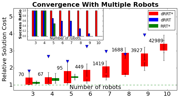
Figure 7 shows the inability of alternatives to compete with ${\tt dRRT^{*}}$ in scalability. Solution costs are normalized by an optimistic estimate of the path cost for each case, which is the sum of the optimal solutions for each robot, disregarding robot-robot interactions. Implicit $\tt A^{\text{*}}$ fails to return solutions even for 3 robots. Directly executing $\tt RRT^{\text{*}}$ in the composite space fails to do so for $R\geq 6$. The original ${\tt dRRT}$ method (without the informed search component) starts suffering in success ratio for $R\geq 5$ and returns worse solutions than ${\tt dRRT^{*}}$. The average solution times for ${\tt dRRT}$ may decrease as $R$ increases but this is due to the decreasing success ratio, i.e., ${\tt dRRT}$ begins to only succeed at easy problems.

Dual-arm manipulator: This test shows the benefits of ${\tt dRRT^{*}}$ when planing for two $7$-dimensional arms. Figure 8 shows that $\tt RRT^{\text{*}}$ fails to return solutions within $100K$ iterations. Using small roadmaps is also insufficient for this problem. Both ${\tt dRRT^{*}}$ and Implicit $\tt A^{\text{*}}$ require larger roadmaps to begin succeeding. But with $N\geq 500$, Implicit $\tt A^{\text{*}}$ always fails, while ${\tt dRRT^{*}}$ maintains a $100\%$ success ratio. As expected, roadmaps of increasing size result in higher quality path. The informed nature of ${\tt dRRT^{*}}$ also allows to find initial solutions fast, which together with the branch-and-bound primitive allows for good convergence.

This work studies the asymptotic optimality of sampling-based multi-robot planning over implicit structures. The objective is to efficiently search the composite space of multi-robot systems while also achieving formal guarantees. This requires construction of asymptotically optimal individual robot roadmaps and appropriately searching their tensor product. Performance is further improved by informed search in the composite space.

These results may extend to more complex settings involving kinodynamic constraints by relying on recent work [14, 13]. Furthermore, the analysis may be valid for different cost functions other than total distance. The tools presented here can prove useful in the context of simultaneous task and motion planning for multiple robots, especially manipulators [1].

References

- [1] A. Dobson and K. E. Bekris. Planning Representations and Algorithms for Prehensile Multi-Arm Manipulation. In IEEE/RSJ International Conference on Intelligent Robots and Systems (IROS), 2015.
- [2] A. Dobson, G. Moustakides, and K. E. Bekris. Geometric Probability Results For Bounding Path Quality In Sampling-Based Roadmaps After Finite Computation. In IEEE Inter. Conf. on Robotics and Automation (ICRA), 2015.
- [3] M. Gharbi, J. Cortés, and T. Siméon. Roadmap Composition for Multi-Arm Systems Path Planning. In IEEE/RSJ International Conference on Intelligent Robots and Systems (IROS), 2009.
- [4] F. Gravot and R. Alami. A Method for Handling Multiple Roadmaps and Its Use for Complex Manipulation Planning. In IEEE Internation Conference on Robotics and Automation (ICRA), 2003.
- [5] C. Grinstead and J. Snell. Introduction to Probability. American Mathmatical Society, Providence, RI, 2012.
- [6] L. Janson, A. Schmerling, A. Clark, and M. Pavone. Fast Marching Tree: a Fast marching Sampling-Based Method for Optimal Motion Planning in Many Dimensions. International Journal of Robotics Research (IJRR), 34(7):883–921, 2015.
- [7] S. Karaman and E. Frazzoli. Sampling-based Algorithms for Optimal Motion Planning. International Journal of Robotics Research (IJRR), 30(7):846–894, June 2011.
- [8] L. E. Kavraki, P. Svestka, J.-C. Latombe, and M. Overmars. Probabilistic Roadmaps for Path Planning in High-Dimensional Configuration Spaces. IEEE Transactions on Robotics and Automation, 12(4):566–580, 1996.
- [9] S. M. LaValle and J. J. Kuffner. Randomized Kinodynamic Planning. International Journal of Robotics Research (IJRR), 20:378–400, May 2001.
- [10] S. Leroy, J. Laumond, and Siméon. Multiple Path Coordination for Mobile Robots: A Geometric Algorithm. Barcelona, Catalonia, Spain, 1999. International Joint Conference on Artificial Intelligence (IJCAI).
- [11] S. R. Lindemann and S. M. LaValle. Incrementally reducing dispersion by increasing voronoi bias in rrts. In Proceedings of the 2004 IEEE International Conference on Robotics and Automation, ICRA 2004, April 26 - May 1, 2004, New Orleans, LA, USA, pages 3251–3257, 2004.
- [12] J. Peng and S. Akella. Coordinating Multiple Robots with Kinodynamic Constraints Along Specified Paths. The International Journal of Robotics Research, 24(4):295–310, 2005.
- [13] E. Schmerling, L. Janson, and M. Pavone. Optimal sampling-based motion planning under differential constraints: The drift case with linear affine dynamics. In 54th IEEE Conference on Decision and Control, CDC 2015, Osaka, Japan, December 15-18, 2015, pages 2574–2581, 2015.
- [14] E. Schmerling, L. Janson, and M. Pavone. Optimal sampling-based motion planning under differential constraints: The driftless case. In IEEE International Conference on Robotics and Automation, ICRA 2015, Seattle, WA, USA, 26-30 May, 2015, pages 2368–2375, 2015.
- [15] J. T. Schwartz and M. Sharir. On the Piano Movers’ Problem: III. Coordinating the Motion of Several Independent Bodies: The Special Case of Circular Bodies Moving Amidst Polygonal Barriers. The International Journal of Robotics Research, 2(3):46–75, 1983.
- [16] K. Solovey, O. Salzman, and D. Halperin. Finding a needle in an exponential haystack: Discrete RRT for exploration of implicit roadmaps in multi-robot motion planning. I. J. Robotics Res., 35(5):501–513, 2016.
- [17] K. Solovey, O. Salzman, and D. Halperin. New Perspective on Sampling-based Motion Planning via Random Geometric Graphs. In Robotics Science and Systems (RSS), 2016.
- [18] P. Svestka and M. Overmars. Coordinated Path Planning for Multiple Robots. Robotics and Autonomous Systems, 23:125–152, 1998.
- [19] S. Tang and V. Kumar. A Complete Algorithm for Generating Safe Trajectories for Multi-Robot Teams. In International Symposium on Robotics Research (ISRR), Sestri Levante, Italy, September 2015.
- [20] J. Van Den Berg, S. Guy, M. Lin, and D. Manocha. Reciprocal n-body collision avoidance, volume 70 of Springer Tracts in Advanced Robotics, pages 3–19. Star edition, 2011.
- [21] J. van den Berg, J. Snoeyink, M. Lin, and D. Manocha. Centralized Path Planning for Multiple Robots: Optimal Decoupling into Sequential Plans. In Robotics: Science and Systems (RSS), 2009.
- [22] G. Wagner and H. Choset. Subdimensional Expansion for Multirobot Path Planning. Artificial Intelligence Journal, 219:1024, 2015.
-A Proof of Convergence
This appendix examines the result of Theorem 2, and formally proves the convergence of the tree toward containing all optimal paths.
Lemma 2 (Optimal Tree Convergence of )
Consider an arbitrary optimal path originating from and ending at , then let be the event such that after iterations of , the search tree contains the optimal path up to segment . Then,
Proof. This property will be proven using a theorem from Markov chain literature [5, Theorem 11.3]. Specifically, the properties of absorbing Markov chains can be exploited to show that will eventually contain the optimal path over for a given query. An absorbing Markov chain is one such that there is some subset of states in which the transition matrix only allows that state to transition to itself.
The proof follows by showing that the method can be described as an absorbing Markov chain, where the target state of a query is represented as an absorbing state in a Markov chain, re-stated here.
Theorem 3 (Thm 11.3 in Grinstead & Snell)
In an absorbing Markov chain, the probability that the process will be absorbed is 1 (i.e., as ), where is the transition submatrix for all non-absorbing states.
There are two steps to using this proof. First, that the search can be cast as an absorbing Markov chain, and second, that the probability of transition for from each state to the next in this chain is nonzero (i.e. that each state can eventually be connected to the target).
For query , let the sequence of length represent the vertices of corresponding to the optimal path through the graph which connects these points, where corresponds to the target vertex, and furthermore, let be an absorbing state. Theorem 3 operates under the assumption that each vertex is connected to an absorbing state ( in this case).
Then, let the transition probability for each state have two values, one for each state transitioning to itself, which corresponds to the search expanding along some other arbitrary path. The other value is a transition probability from to . This corresponds to the method sampling within the volume .
Then, as the second step, it must be shown that this volume has a positive probability of being sampled in each iteration. It is sufficient then to argue that . Fortunately, for any finite , previous work has already shown that this is the case given general position assumptions [16, Lemma 2].
Given these results, the is cast as an absorbing Markov chain which satisfies the assumptions of 3, and therefore, the matrix . This implies that the optimal path to the goal has been expanded in the tree, and therefore ∎
-B More Experimental Data
This appendix presents additional experimental data omitted from Section V.
-B1 2-Robot Benchmark
For the two-robot benchmark, additional data is presented in Figure 9. Here, the data presented in Figure 6 is shown again over time instead of over iterations.
-B2 R-Robot Benchmark
For the -robot benchmark, additional data is presented in Figure 10, showing query resolution times for the various methods.
To emphasize the lack of scalability for alternate methods, additional experiments were run in this setup using a minimal roadmap. The tests use a -node roadmap for each robot as illustrated in Figure 12. Each roadmap is constructed with slight perturbations to the nodes within the shaded regions indicated in the figure.
The data for this modified benchmark (shown in Figure 11) indicate that even using a very small roadmap does not allow alternate methods to scale. While the methods scale better, Implict does time out for , and times out for .
-B3 Manipulator Benchmark
For the dual-arm manipulator benchmark, additional data is presented in Figure 13. Here, the data of Figure 8 is shown over iterations instead of over time.