A study of the dense Uniform Electron Gas with high orders of Coupled Cluster
Abstract
We investigate the accuracies of different coupled cluster levels in a finite model solid, the 14 electron spin-non-polarised uniform electron gas. For densities between 0.5 and 5 , we calculate ground state correlation energies with stochastic coupled cluster ranging from coupled cluster singles and doubles (CCSD) to coupled cluster including all excitations up to quintuples (CCSDTQ5). We find the need to add triple excitations for an accuracy of 0.01eV/electron beyond 0.5 . Quadruple excitations start being significant past 3 . At 5 , CCSD gives a correlation energy with a 16% error and CCSDT is in error by 2% compared to the CCSDTQ5 result. CCSDTQ5 gives an energy in agreement with full configuration interaction quantum Monte Carlo results.
pacs
05.10.Ln,02.70.Ss,31.15.bw,31.15.V-,71.10.CaI Introduction
Coupled cluster theory [1, 2, 3] is known as the gold standard of ab initio molecular simulations giving energies to chemical accuracy of about 1 kcal mol-1 (see review Ref. 4). Moreover, its accuracy is systematically improvable as more excitation levels are added. Driven by the need for systematically improvable methods in solids, coupled cluster is now increasingly being applied to periodic systems, see e.g. Refs. 5, 6, 7, 8, 9, 10, 11, 12. In this paper we apply the stochastic coupled cluster method [13, 14] to the dense uniform electron gas to assess the performance of coupled cluster in periodic systems at representative electron densities. Performing coupled cluster stochastically can often reduce the memory requirements and computational scaling. It can therefore reach higher basis sets and coupled cluster levels than conventional implementations.
While coupled cluster is just starting to emerge as a useful tool for solid calculations, density functional theory (DFT) [15, 16] is one of the most widely used ab initio electronic structure methods in extended systems. It scales favourably (() or even () (see e.g. Ref. 17) where is a measure for the system size) but it is not systematically improvable and it can have difficulties with strongly correlated systems [18]. These and other shortcomings have led to an interest in applying alternative methods to periodic systems. Besides coupled cluster, these include for example the random phase approximation (RPA) [19, 20, 21], second order Møller-Plesset perturbation theory (MP2) [22], diffusion Monte Carlo (DMC) [23] and (initiator) full configuration interaction quantum Monte Carlo (FCIQMC) [24, 25, 8]. RPA yields a ground state energy that is equal to the energy output of a version of ring diagram coupled cluster doubles (CCD) [26, 27]. MP2 has been shown to diverge in the thermodynamic limit in the uniform electron gas whereas it is unclear whether coupled cluster singles and doubles (CCSD) does [28, 29]. DMC scales as () [23] and can give the exact answer provided sufficient a priori information about the wavefunction is available. FCIQMC gives exact energies within a finite basis set without requiring a priori knowledge of the wavefunction. Most such calculations are now performed with the initiator approximation [25] that adds a bias to the energy which can be systematically reduced as more Monte Carlo particles are added to the system. FCIQMC has so far been applied to small systems, including LiH (333 point mesh with 2 electrons and 2 orbitals per point) and diamond (222 points with 8 electrons and 8 orbitals per point) [8]. Since FCIQMC samples the whole Hilbert space, it is often more expensive than a level of coupled cluster that is sufficient for accurate energies.
The system we study here is the uniform electron gas (UEG) [30, 31, 32] which is a simple model for a periodic system where the positive lattice potential of the atomic nuclei is approximated by a uniform positive background potential; the energies of electron gases play an important role in density functional theory [31, 33, 32]. There exists accurate ground state energy data for the high density regime based on the finite UEG with the FCIQMC [34, 35, 36] and DMC [37, 38, 39, 40, 41, 42, 43, 44, 45] methods. Versions of coupled cluster have been applied to the UEG in the thermodynamic limit, see e.g. [26, 46, 47]. CCSD and CCSDT have been applied to the finite three-dimensional (3D) UEG [34, 29, 48, 14, 49, 50]. Shepherd [50] has extrapolated finite CCSD/CCD results in the 3D UEG to the thermodynamic limit and has compared them to Ceperley and Alder’s DMC energies [37] (see figure 2c in Ref. 50). Using these DMC energies as a reference, the extrapolated CCSD correlation energy has an error of under 10% at 1.0 which increases to about 20% at 5.0 . Another recent study [14] has performed initiator and non-initiator stochastic coupled cluster in the CCSD and CCSDT levels on the dense 14 electron 3D UEG. The difference between CCSD and CCSDT was found to be significant even in the low correlation regime at 1.0 . is the radius of a sphere that on average contains one electron. In this paper, we apply coupled cluster up to the CCSDTQ5 level which included quintuple excitations directly to the 14 electron non-spin-polarized UEG in the range 0.5 to 5.0 which is representative of some common simple solids (e.g. see Ref. 30). We compare with (initiator) FCIQMC [36] and MP2 [34] results. Using coupled cluster levels from CCSD to CCSDTQ5, we aim to answer the question what coupled cluster level is needed to accurately model simple finite solids with certain densities, represented by the parameter, with coupled cluster.
II Coupled Cluster Monte Carlo
Coupled Cluster Monte Carlo (CCMC) [13, 14] is a stochastic version of the coupled cluster method [1, 2, 3, 4]. The energies obtained are consistent with conventional coupled cluster while often saving computational and memory cost [13, 14, 51]. Recent developments include linked CCMC [52], the initiator approximation for CCMC [14] and the even selection feature [51]. This section gives a brief overview over the method which is described more thoroughly in the literature [13, 14].
Coupled cluster theory solves the Schrödinger equation for the ground state energy. The ground state wavefunction is constructed from the reference wavefunction using the ansatz
| (1) |
where . Wavefunctions are expressed in a Slater determinant basis. In this study, , the Hartree-Fock Slater determinant. are excitors, that produce excited Slater determinants . are the corresponding coefficients of . If the sum is over all possible , will tend to the full configuration interaction (FCI) wavefunction. Coupled cluster theory has the advantage over doing (F)CI that it can truncate the sum for to only include some excitors while still being size consistent. Coupled cluster singles and doubles (CCSD) for example only includes excitors that excite one or two electrons whereas CCSDT also includes excitors that excite three electrons from the reference and so on. Due to the exponential in equation 1, higher order excitations are still present indirectly, created by a combination of lower order ones and therefore dependent on their coefficients .
Stochastic Coupled Cluster makes use of the sparsity of the wavefunction, and uses sampling to decrease computational and memory costs. To understand the sampling algorithm, we first project the Schrödinger equation onto some determinant giving a set of equations
| (2) |
Instead of explicitly solving these equations, the ground state wavefunction is formed by a projection from the reference, , where imaginary time, . After some manipulation, [13, 14] this yields an iterative equation for the amplitudes ,
| (3) |
Monte Carlo particles are placed on the excitors . They are then propagated to sample equation 3 which is explained in more detail in the following paragraph. At convergence, the average population on an excitor corresponds to its coefficient . These particles do not have to be discrete and can take real-valued weights [53, 54].
We start the Monte Carlo sampling by randomly picking a cluster (i.e. a combination) of excitors that are occupied by particles. They act on the reference determinant to yield an excited determinant . The three major steps are [13, 24]:
- •
Spawn: Another determinant that may be unoccupied or occupied is randomly chosen. With a probability proportional to , Monte Carlo particles can spawn to .
- •
Death/Birth: With a probability proportional to a particle is placed on . is the population-controlling shift, described below, and is the Hartree-Fock energy.
- •
Annihilation: Finally, particles of opposite sign on the same excitor are removed.
The ground state correlation energy is estimated by the projected energy
| (4) |
and, independently, by the above-mentioned shift. The shift is usually set to zero at the beginning and when the particle number is high enough (when we have passed the plateau phase of the sampling [13, 55]) it is varied as [24]
| (5) |
where is a damping parameter and is the number of iterations to pass before the shift is updated.
Franklin et al. [52] have modified equation 3 (which later had replaced by the sum of the shift and the Hartree Fock energy ) to
| (6) |
which we use as well. We use equation 4 to find an estimate of for . This change does not affect the Spawn and Annihilation steps. If a single excitor was selected before the Spawn step, the (modified) Death/Birth step causes a particle to die/be created on with a probability proportional to . For composite clusters, i.e. if two or more excitors were selected and collapsed to , the probability is proportional to instead as we do not sample the third term on the right hand side of equation 6 then.
For our stochastic calculations, we have made use of development versions of the HANDE code 11 1 See Ref. 69 and http://www.hande.org.uk/ for information and code.. We have used the cluster multispawn feature [57] and the full non-composite cluster selection described in Ref. 57 using one MPI process divided up into OpenMP threads when running CCMC. We have also run some FCIQMC calculations to compare our CCMC results to and we used the conventional and initiator versions for FCIQMC [24, 25] while only using non-initiator CCMC. The error bars of the data presented here were estimated by reblocking analysis [58] using pyblock 22 2 See https://github.com/jsspencer/pyblock for information and code. and the correlation energies are obtained from the projected energy. For the data presented here, the projected energy agrees with the shift within 2. Errors were combined in quadrature. We found no significant population control bias using a reweighting scheme used in DMC [60] and adapted to FCIQMC [61].
III Uniform Electron Gas
We used a plane wave basis and studied the 14 electron non-spin-polarised electron gas. The simulation was performed in three dimensional space, where the set of are the wavevectors of the plane waves, with a cubic simulation box with sides of length . A kinetic energy cutoff was used to select the plane waves. In space and using second quantisation, the Hamiltonian is expressed as
| (7) |
/ creates/annihilates an electron with momentum and is the Madelung constant that does not affect the correlation energy. where is the number of electrons.
IV Extrapolation to Complete Basis Set Limit
Coupled cluster singles and doubles (CCSD) is the least expensive level of coupled cluster. Owing to momentum and spin conservation, CCSD is equivalent to CCD in the UEG. At first, we extrapolated CCSD calculations to the complete basis set (CBS) limit for the 14 electron UEG. We then estimated the CBS limit of the other truncation levels studied by extrapolating energy differences between truncation levels and adding this to the CBS CCSD result. This is similar to the idea of focal point analysis as described in e.g. Ref. 62.
Shepherd et al. [34] have shown that for MP2, the correlation energy for a finite basis set with spinorbitals goes as in the leading order for large . They and other studies [35, 36, 63, 64, 50, 14] have used this trend and shown that it also holds reasonably well for CCSD and FCI(QMC). These studies have usually excluded points with larger that were no longer in the region in which is a good fit.
In this study, we have decided to modify this approach to allow higher orders of to be considered as well. This accounts for the fact that is merely a leading order term and by adding higher orders we allow for correction terms to account for the part of the energy not accounted for by . There are two aspects that need to be considered when choosing the best fit curve: What polynomial are we fitting, i.e. what is the highest order of to include, and how many points with high should be excluded from the fit?
Starting with the lowest order polynomial to fit ( when fitting CCSD and a constant when fitting coupled cluster differences), we first fit all the data points and then start excluding points with lowest . For each fit, we calculate over number of degrees of freedom #d.o.f.. where is a data value, is its fitted value and is the standard deviation of [65]. As soon as we reach a local minimum in the /#d.o.f. value, we stop removing points and note down the value at = 0 given by the fit at the local minimum. If no local minimum can be found before there are as few data points left as the number of fitting parameters, then the search for a best fit for the first polynomial was unsuccessful. We then repeat this procedure of consecutively removing data points with the next order polynomials, initially starting with a full set of data points again. We fit linear, quadratic and cubic polynomials and a constant as well if we are fitting to differences. Finally, we compare the results of the fits at local minima in the number of points at = 0. If the lowest order fit result agrees with the higher order ones within 2, we accept it as the CBS result. If it does not agree with all the higher ones, we compare the second lowest order fit result to its higher order fit results, etc. This process can continue up comparing the CBS results from the highest two polynomials. If there is still no CBS result at the end, then the extrapolation was not successful and a CBS value has to be estimated (see results section for individual cases).
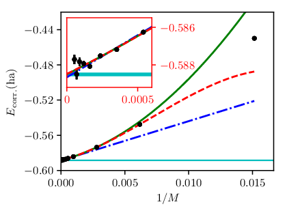
As an example, figure 1 shows the best fits with the lowest #d.o.f. for = 0.5 CCSD and 14 electrons. The linear and the quadratic fit intercepts do not agree within 2. The quadratic and cubic fits agree which meant that we took the quadratic fit intercept as the CBS result. We have used the curve_fit function in the SciPy 33 3 E. Jones, T. Oliphant, P. Peterson et al., SciPy: Open source scientific tools for Python. See https://www.scipy.org/ for more information. optimize module for curve fitting and Matplotlib [67] for plotting. The standard errors of the correlation energy were treated as absolute and not relative weights.
V Results
Figure 2 shows how the differences in correlation energy between consecutive coupled cluster levels vary with for different numbers of spinorbitals . As a reference, an accuracy of 0.01 eV/electron = 0.00037 ha/electron is shown with dashed horizontal lines. This is of a similar order of magnitude as chemical accuracy (ca. 0.04 eV/molecule [23]). To distinguish solid phases from each other, enthalpy differences of about 0.1 eV/atom often need to be resolved and at room temperature an accuracy of 0.01 eV in the energy is desired (see Ref. 68 for details). We have therefore chosen 0.01 eV/electron as a guide for energies to be of sufficient accuracy.


The CCSD to CCSDTQ5 CBS values are summarized in table 1. Note that while figure 2 quotes energies in energies per electron, table 1 shows energies for 14 electrons. First, the CCSD CBS value was found and then the CBS limit of differences between consecutive coupled cluster levels were added on to find the CBS limit of the other truncation levels. For up to 2.0 , earlier CCSD and CCSDT results [14] are shown as well. MP2 results [34] and FCIQMC are given for comparison. For = 0.5, 1.0, 2.0 and 5.0 FCIQMC values from Shepherd et al. [36] are given and additionally for = 0.5 and 1.0 , new FCIQMC CBS results are presented for comparison. When using the initiator approximation [25], the FCIQMC correlation energies values for a certain number of spinorbitals were estimated by fitting horizontal lines to energy against number of Monte Carlo particles curves, consecutively removing data points with the least number of particles. The energy at the global minimum in #d.o.f. when fitting a horizontal line is taken as the energy result. The error in the average number of particles was very small and therefore ignored. For the (i)FCIQMC results with = 0.5 and 1.0 , the initiator approximation was used for greater then 358 and 66 respectively. The initiator method was not used for CCMC calculations in this study.
| = 0.5 | = 1.0 | = 2.0 | = 3.0 | = 5.0 | |
|---|---|---|---|---|---|
| CCSD | -0.58850(6)/-0.5897(1)44 4 This (initator) CCSD/CCSDT value is from Spencer et al.[14] | -0.51450(9)/-0.5155(3)11footnotemark: 1 55 5 Also compare to -0.5152(5) from figure 7 in Shepherd et al.[34] as quoted by Spencer et al. [14] | -0.4096(10)/-0.4094(1)11footnotemark: 1 | -0.3395(1) | -0.2531(3) |
| CCSDT | -0.59457(7)/-0.5965(2)11footnotemark: 1 | -0.5307(2)/-0.5317(3)11footnotemark: 1 | -0.4407(10)/-0.4354(4)11footnotemark: 1 | -0.3780(3)66 6 The CCSDT to CCSD energy difference for = 3.0 was estimated by the mean of a constant, linear, quadratic and cubic fit with lowest #d.o.f. if multiple fits were available. | -0.2970(4)77 7 The CCSDT to CCSD energy difference for = 5.0 was estimated by the mean of a constant, linear and quadratic fit with lowest #d.o.f. if multiple fits were available. |
| CCSDTQ | -0.59465(8) | -0.5311(2) | -0.4432(10)88 8 The CCSDTQ to CCSDT difference for = 2.0 and 3.0 and the CCSDTQ5 to CCSDTQ difference for = 0.5 was estimated by the mean of a linear fit and the data point with lowest . | -0.3833(3)33footnotemark: 3 55footnotemark: 5 | -0.3015(4)44footnotemark: 4 99 9 The CCSDTQ to CCSDT difference for = 5.0 and the CCSDTQ5 to CCSDTQ difference for = 1.0, 2.0, 3.0 and 5.0 was estimated by the CCSDTQ to CCSDT difference at 66 spinorbitals. |
| CCSDTQ5 | -0.5947(2)55footnotemark: 5 | -0.5311(2)66footnotemark: 6 | -0.4434(10)55footnotemark: 5 66footnotemark: 6 | -0.3837(3)33footnotemark: 3 55footnotemark: 5 66footnotemark: 6 | -0.3025(4)44footnotemark: 4 66footnotemark: 6 |
| FCIQMC | -0.59467(9)1010 10 (i)FCIQMC value of = 0.5 was estimated by the CCSDTQ value plus the difference of CCSDTQ to (i)FCIQMC extrapolated value./-0.5969(3)1111 11 This iFCIQMC data is from Shepherd et al. [36] | -0.5313(2)1212 12 (i)FCIQMC value of = 1.0 was estimated by the CCSDT value plus the difference of CCSDT to (i)FCIQMC extrapolated value./-0.5325(4)88footnotemark: 8 | -0.4447(4)88footnotemark: 8 | -0.306(1)88footnotemark: 8 | |
| MP2 | -0.575442(1)1313 13 The MP2 data is from Shepherd et al. [34] | -0.499338(2)1010footnotemark: 10 | -0.398948(2)1010footnotemark: 10 | -0.255664(4)1010footnotemark: 10 |
VI Discussion
Figure 2(a) shows that CCSD gives an accuracy worse than 0.01 eV/electron for greater than 0.5 as the difference between CCSD and CCSDT is greater than 0.01 eV/electron. Considering figure 2(b), CCSDT seems to be sufficient up to = 2.0 . As the differences in correlation energy increase in magnitude with and the = 162 energy for = 3.0 is close to 0.01 eV/electron, one should be cautious about using CCSDT for = 3.0 . Figure 2(c) shows that the difference between CCSDTQ and CCSDTQ5 is not negligible for greater than 2.0 .
Of course, this analysis implicitly assumes that the energy is monotonically decreasing with coupled cluster level. If the difference to the next excitation level is bigger than 0.01 eV/electron, we expect the difference to the true energy also to be greater than 0.01 eV/electron. However, we found that in our case, the energy was monotonically decreasing and the CCSDTQ5 result agrees very well with FCIQMC, see table 1. This supports our approach of comparing the energy difference to the next excitation level when assessing accuracies.
Figure 3 shows the difference in correlation energy found with CCSD, CCSDT and CCSDTQ to the correlation energy found with CCSDTQ5 as a fraction of the CCSDTQ5 correlation energy. Given that the CCSDTQ5 energy shown in table 1 is merely a lower bound for the true magnitude of the CCSDTQ5 energy, the errors presented here are also lower bounds. The error in CCSD is at least 16% for = 5.0 and for CCSDT it is still as big as about 2%. The error of CCSDTQ is small but noticable for = 5.0 . This means that for a study of a solid with 4 say, e.g. sodium, CCSD may give a correlation energy that is off by over 12% and the error with CCSDT is still over 1%. As the energy differences between coupled cluster levels increase with , properties such as the lattice parameter or the bulk modulus will be underestimated by low orders of coupled cluster.

As Shepherd et al.[34] already noted, for low , MP2 performs worse than CCSD and vice versa for higher in the regime studied (see table 1). MP2 gives a less accurate answer than CCSDT and higher truncation levels for all studied .
We present new extrapolated FCIQMC results for = 0.5 and 1.0 , which are similar to but do not agree with Shepherd et al.’s [36] values. Similarly, our CCSD and CCSDT values for = 0.5 and 1.0 do not agree within 2 with Spencer et al.’s [14] values. Our CBS correlation energies are less negative. We can explain these deviations by considering the shape of the extrapolation curves such as figure 1. Our CCSD calculations went up to 18342/11150 spinorbitals for = 0.5/1.0 and that was our starting point to extrapolate higher truncations and FCIQMC from. Shepherd et al. [36] and Spencer et al. [14] only considered up to 4218 at most. If fewer data points with low are present and a linear fit is employed (as Shepherd et al. [36] and Spencer et al. [14] did), the intercept with the axis, the CBS energy estimate, will be more negative than in the case where lower are present and higher fits are allowed. Our FCIQMC values quoted in table 1 were found by extrapolating the difference between the CCSDTQ/CCSDT and the FCIQMC values for = 0.5/1.0 as CCSDTQ/CCSDT was the highest coupled cluster data set that contained the highest used in our FCIQMC study for = 0.5/1.0 respectively. Had we instead extrapolated FCIQMC directly, the results would have been -0.59497(4) ha (instead of -0.59467(9) ha) with a linear fit for = 0.5. For this direct fit we included spinorbitals up to = 4218 and when we extrapolated differences, we used information from the CCSD result with spinorbitals up to 18342. This shows that it is crucial to include large numbers of virtual orbitals to converge to the correct answer. We believe that the disagreement of the CCSD and CCSDT values for = 0.5 and 1.0 with Spencer et al.’s [14] values may also be due to initiator energies that are not converged fully. We have not used the initiator approximation for coupled cluster data here.
VII Summary and Conclusions
We have shown that CCSD and CCSDT are limited for modelling finite solids that can be described by the 14 electron uniform electron gas with greater than 2.0 . A comparison with CCSDTQ5 has shown that if an accuracy of 0.01 eV/electron is desired, CCSDT is required beyond = 0.5 and CCSDTQ is worth considering beyond = 3.0 . At = 5.0 , CCSD only reproduces up to about 84% of the correlation energy and CCSDT up to about 98%.
This study has demonstrated that there can be a need for coupled cluster orders beyond CCSDT when modelling finite correlated solid-state systems.
Acknowledgements.
We thank Dr. Pablo López Ríos for helpful discussions on fitting, especially the idea of using (number of degrees of freedom). For the research data supporting this publication and more information, see https://doi.org/10.17863/CAM.14336. V.A.N. would like to acknowledge the EPSRC Centre for Doctoral Training in Computational Methods for Materials Science for funding under grant number EP/L015552/1. A.J.W.T. thanks the Royal Society for a University Research Fellowship under grant UF110161. This work used the UK Research Data Facility (http://www.archer.ac.uk/documentation/rdf-guide) and ARCHER UK National Supercomputing Service (http://www.archer.ac.uk) under ARCHER Leadership project with grant e507.References
- [1] F. Coester and H. Kümmel, Nucl. Phys. 17, 477 (1960).
- [2] J. Čižek, J. Chem. Phys. 45, 4256 (1966).
- [3] J. Čižek and J. Paldus, Int. J. Quantum Chem. 5, 359 (1971).
- [4] R. J. Bartlett and M. Musiał, Rev. Mod. Phys. 79, 291 (2007).
- [5] S. Hirata, I. Grabowski, M. Tobita, and R. J. Bartlett, Chem. Phys. Lett. 345, 475 (2001).
- [6] S. Hirata, R. Podeszwa, M. Tobita, and R. J. Bartlett, J. Chem. Phys. 120, 2581 (2004).
- [7] A. Grüneis, G. H. Booth, M. Marsman, J. Spencer, A. Alavi, and G. Kresse, J. Chem. Theory Comput. 7, 2780 (2011).
- [8] G. H. Booth, A. Grüneis, G. Kresse, and A. Alavi, Nature 493, 365 (2013).
- [9] A. Grüneis, J. Chem. Phys. 143, 102817 (2015a).
- [10] A. Grüneis, Phys. Rev. Lett. 115, 066402 (2015b).
- [11] K. Liao and A. Grüneis, J. Chem. Phys. 145, 141102 (2016).
- [12] J. McClain, Q. Sun, G. K.-L. Chan, and T. C. Berkelbach, J. Chem. Theory Comput. 13, 1209 (2017), arXiv:1701.04832 .
- [13] A. J. W. Thom, Phys. Rev. Lett. 105, 263004 (2010).
- [14] J. S. Spencer and A. J. W. Thom, J. Chem. Phys. 144, 084108 (2016), arXiv:1511.05752 .
- [15] W. Kohn and L. J. Sham, Phys. Rev. 140, A1133 (1965).
- [16] P. Hohenberg and W. Kohn, Phys. Rev. 136, B864 (1964).
- [17] C.-K. Skylaris, P. D. Haynes, A. A. Mostofi, and M. C. Payne, J. Chem. Phys. 122, 084119 (2005).
- [18] A. J. Cohen, P. Mori-Sánchez, and W. Yang, Chem. Rev. 112, 289 (2012).
- [19] D. Bohm and D. Pines, Phys. Rev. 82, 625 (1951).
- [20] D. Pines and D. Bohm, Phys. Rev. 85, 338 (1952).
- [21] D. Bohm and D. Pines, Phys. Rev. 92, 609 (1953).
- [22] C. Møller and M. S. Plesset, Phys. Rev. 46, 618 (1934).
- [23] W. M. C. Foulkes, L. Mitas, R. J. Needs, and G. Rajagopal, Rev. Mod. Phys. 73, 33 (2001).
- [24] G. H. Booth, A. J. W. Thom, and A. Alavi, J. Chem. Phys. 131, 054106 (2009).
- [25] D. Cleland, G. H. Booth, and A. Alavi, J. Chem. Phys. 132, 041103 (2010).
- [26] D. L. Freeman, Phys. Rev. B 15, 5512 (1977), arXiv:arXiv:1011.1669v3 .
- [27] G. E. Scuseria, T. M. Henderson, and D. C. Sorensen, J. Chem. Phys. 129, 231101 (2008).
- [28] J. J. Shepherd and A. Grüneis, arXiv[physics.chem-ph] (2012), arXiv:1208.6103v1 .
- [29] J. J. Shepherd and A. Grüneis, Phys. Rev. Lett. 110, 226401 (2013), arXiv:1310.6059 .
- [30] R. M. Martin, in Electron. Struct. (Cambridge University Press, Cambridge, 2004) pp. 100–118.
- [31] G. Giuliani and G. Vignale, in Quantum Theory Electron Liq. (Cambridge University Press, Cambridge, 2005) pp. 1–68.
- [32] P.-F. Loos and P. M. W. Gill, WIREs Comput. Mol. Sci. 6, 410 (2016), arXiv:1601.03544 .
- [33] G. Giuliani and G. Vignale, in Quantum Theory Electron Liq. (Cambridge University Press, Cambridge, 2005) pp. 327–404.
- [34] J. J. Shepherd, A. Grüneis, G. H. Booth, G. Kresse, and A. Alavi, Phys. Rev. B 86, 035111 (2012a), arXiv:1202.4990 .
- [35] J. J. Shepherd, G. Booth, A. Grüneis, and A. Alavi, Phys. Rev. B 85, 081103 (2012b), arXiv:1109.2635 .
- [36] J. J. Shepherd, G. H. Booth, and A. Alavi, J. Chem. Phys. 136, 244101 (2012c), arXiv:1201.4691 .
- [37] D. M. Ceperley and B. J. Alder, Phys. Rev. Lett. 45, 566 (1980).
- [38] G. Ortiz and P. Ballone, Phys. Rev. B 50, 1391 (1994).
- [39] G. Ortiz and P. Ballone, Phys. Rev. B 56, 9970 (1997).
- [40] G. Ortiz, M. Harris, and P. Ballone, Phys. Rev. Lett. 82, 5317 (1999).
- [41] Y. Kwon, D. M. Ceperley, and R. M. Martin, Phys. Rev. B 58, 6800 (1998).
- [42] M. Holzmann, D. M. Ceperley, C. Pierleoni, and K. Esler, Phys. Rev. E 68, 046707 (2003).
- [43] P. López Ríos, A. Ma, N. D. Drummond, M. D. Towler, and R. J. Needs, Phys. Rev. E - Stat. Nonlinear, Soft Matter Phys. 74, 066701 (2006), arXiv:0801.0518 .
- [44] N. D. Drummond, R. J. Needs, A. Sorouri, and W. M. C. Foulkes, Phys. Rev. B - Condens. Matter Mater. Phys. 78, 125106 (2008), arXiv:0806.0957 .
- [45] G. G. Spink, R. J. Needs, and N. D. Drummond, Phys. Rev. B 88, 085121 (2013), arXiv:1307.5794 .
- [46] R. F. Bishop and K. H. Lührmann, Phys. Rev. B 17, 3757 (1978).
- [47] R. F. Bishop and K. H. Lührmann, Phys. Rev. B 26, 5523 (1982).
- [48] A. Roggero, A. Mukherjee, and F. Pederiva, Phys. Rev. B 88, 115138 (2013), arXiv:1304.1549 .
- [49] J. McClain, J. Lischner, T. Watson, D. A. Matthews, E. Ronca, S. G. Louie, T. C. Berkelbach, and G. K.-L. Chan, Phys. Rev. B 93, 235139 (2016), arXiv:1512.04556 .
- [50] J. J. Shepherd, J. Chem. Phys. 145, 031104 (2016), arXiv:1605.05699 .
- [51] C. J. C. Scott and A. J. W. Thom, J. Chem. Phys. 147, 124105 (2017), arXiv:1706.07017 .
- [52] R. S. T. Franklin, J. S. Spencer, A. Zoccante, and A. J. W. Thom, J. Chem. Phys. 144, 044111 (2016), arXiv:1511.08129 .
- [53] F. R. Petruzielo, A. A. Holmes, H. J. Changlani, M. P. Nightingale, and C. J. Umrigar, Phys. Rev. Lett. 109, 230201 (2012).
- [54] C. Overy, G. H. Booth, N. S. Blunt, J. J. Shepherd, D. Cleland, and A. Alavi, J. Chem. Phys. 141, 244117 (2014).
- [55] J. S. Spencer, N. S. Blunt, and W. M. Foulkes, J. Chem. Phys. 136, 054110 (2012), arXiv:1110.5479 .
- [56] See Ref. \rev@citealpnumHANDEpaper and http://www.hande.org.uk/ for information and code.
- [57] J. S. Spencer, R. S. T. Franklin, V. A. Neufeld, W. A. Vigor, and A. J. W. Thom, (unpublished) .
- [58] H. Flyvbjerg and H. G. Petersen, J. Chem. Phys. 91, 461 (1989).
- [59] See https://github.com/jsspencer/pyblock for information and code.
- [60] C. J. Umrigar, M. P. Nightingale, and K. J. Runge, J. Chem. Phys. 99, 2865 (1993).
- [61] W. A. Vigor, J. S. Spencer, M. J. Bearpark, and A. J. W. Thom, J. Chem. Phys. 142, 104101 (2015), arXiv:1407.1753 .
- [62] A. L. L. East and W. D. Allen, J. Chem. Phys. 99, 4638 (1993).
- [63] J. J. Shepherd, T. M. Henderson, and G. E. Scuseria, J. Chem. Phys. 140, 124102 (2014a), arXiv:1310.6806 .
- [64] J. J. Shepherd, T. M. Henderson, and G. E. Scuseria, Phys. Rev. Lett. 112, 133002 (2014b), arXiv:1310.6425 .
- [65] G. McPherson, Stat. Sci. Investig., Springer Texts in Statistics (Springer New York, New York, NY, 1990).
- [66] E. Jones, T. Oliphant, P. Peterson et al., SciPy: Open source scientific tools for Python. See https://www.scipy.org/ for more information.
- [67] J. D. Hunter, Comput. Sci. Eng. 9, 90 (2007).
- [68] L. K. Wagner and D. M. Ceperley, Reports Prog. Phys. 79, 094501 (2016), arXiv:1602.01344 .
- [69] J. S. Spencer, N. S. Blunt, W. A. Vigor, F. D. Malone, W. M. C. Foulkes, J. J. Shepherd, and A. J. W. Thom, J. Open Res. Softw. 3, 1 (2015), arXiv:1407.5407 .