The eagle simulations of galaxy formation:
Public release of particle data
Abstract
This manual accompanies the release of the particle data for 24 simulations of the eagle suite of cosmological hydrodynamical simulations of galaxy formation by the virgo consortium. It describes how to download these snapshots and how to extract datasets from them, emphasising the meaning of variables, and their units. We provide examples for extracting the particle data in python. This data release complements our earlier release of numerous integrated properties of the galaxies in eagle through an sql relational database. This database has been updated to include the additional simulations that are part of the present data release. Scientists wanting to use eagle may find it useful to first investigate whether their analysis can be performed using the database, before accessing the particle data. The particles in the snapshot files are indexed by a peano-hilbert key. This allows for an eased extraction of simply connected spatial volumes, without needing to read the entire snapshot. This makes it possible to analyse many aspects of galaxies using modest computing resources, even when using eagle simulations with large numbers of particles. A reading routine is provided to simplify this process.
1 Introduction
1.1 The eagle simulations
The Virgo consortium’s Evolution and Assembly of GaLaxies and their Environments (hereafter eagle) project consists of a suite of cosmological hydrodynamical simulations designed to enable the study of the formation and evolution of a population of galaxies in a cosmologically representative volume [1, 2], adopting the cosmological parameters advocated by the Planck Collaboration ([3]) (, , , , , , ).
All simulations were performed with the gadget-3 tree-SPH code, which is based on the gadget-2 code described by [4], but extensively modified as described in detail by [1] and references therein. Modifications include changes to the hydrodynamics and time-stepping schemes referred to as anarchy, and the implementation of a large number of ‘subgrid’ modules that account for physical processes below the resolution scale (radiative cooling and heating in the presence of an imposed optically thin radiation background, star formation, stellar evolution, metal enrichment, feedback from stars, seeding and growth by accretion and merging of supermassive black holes and feedback from accreting black holes). These subgrid modules are described by [1] and references therein. Numerical parameters for the eagle reference model associated with the subgrid modules were calibrated to a limited subset of observations of galaxies, namely: the galaxy stellar mass function, the sizes of galaxies, and the black hole mass - stellar mass relation. The motivation for doing so is detailed by [1], with the calibration strategy described in detail by [2].
Simulations were performed in cubic volumes with lengths of , 25, 50 and 100 co-moving mega-parsec (cMpc) on a side, at a range of resolutions. Simulations with an initial baryonic particle mass (SPH mass) of are referred to as ‘high resolution’ and those with an initial baryonic particle mass of referred to as ‘intermediate resolution’. The corresponding (‘Plummer equivalent’) maximum gravitational softening lengths are pkpc (proper kilo-parsec) and 0.70 pkpc respectively, with the code switching to a softening that is a constant, , in co-moving coordinates at . Table 1 summarises these properties for key runs, and illustrates the naming convention, for example L0025N0376 refers to a simulation with cMpc that starts with (dark matter and gas) particles.
In addition to the reference simulations, the eagle suite comprises runs where one or more of the subgrid modules, or parameters of these modules, were changed. The recal model, recalL0025N0752, is calibrated to the same galaxy properties as reference, with the (relatively small) changes to the subgrid parameters as a consequence of the higher resolution compared to the default ‘intermediate resolution’ runs. Other models, e.g, WeakFBL0025N0376 or StrongFBL0025N0376, are not re-calibrated. These variations to subgrid parameters are aimed at understanding the effect of changing parameters one at a time (in the example, the strength of feedback from star formation). The models are summarised in Table 2, with a short description of how they differ from reference.
eagle has generated several spin off projects that use the same (or very similar) simulation code and models. These include zooms of Local Group-like regions (the apostle project described by [5, 6]); zooms of galaxy clusters (the C-eagle and hydrangea projects described by [7, 8]); simulations with warm dark matter [9]; and zooms of Milky Way-like galaxies that include non-equilibrium chemistry [10]. Currently, the data from those spin off projects is not part of this data release. The Virgo consortium releases these particle data in the hope that they will be useful to the community. We are keen to receive feedback and suggestions concerning how this release could be made more useful.
| Name | ||||||
|---|---|---|---|---|---|---|
| (cMpc) | () | () | (ckpc) | (pkpc) | ||
| RefL0025N0376 | 25 | 2.66 | 0.70 | |||
| RecalL0025N0752 | 25 | 1.33 | 0.35 | |||
| RefL0050N0752 | 50 | 2.66 | 0.70 | |||
| RefL0100N1504 | 100 | 2.66 | 0.70 |
| Name | Resolution | Description |
| Small test volume | ||
| RefL0012N0188 | Intermediate | Reference model |
| Models from [1] | ||
| RefL0025N0376 | Intermediate | Reference model |
| RefL0025N0752 | High | Higher resolution version evolved using Reference parameters |
| RecalL0025N0752 | High | Higher resolution version recalibrated to same data as Reference model |
| RefL0050N0752 | Intermediate | Reference model |
| AGNdT9L0050N0752 | Intermediate | Higher AGN heating temperature and lower subgrid black hole accretion disc viscosity |
| RefL0100N1504 | Intermediate | Reference model |
| Models calibrated to the galaxy stellar mass function from [2] | ||
| FBconstL0050N0752 | Intermediate | Constant stellar feedback efficiency |
| FBsigmaL0050N0752 | Intermediate | Stellar feedback dependent on dark matter velocity dispersion |
| FBZL0050N0752 | Intermediate | Stellar feedback dependent only on metallicity (not on density) |
| Model variations from [2] | ||
| eos1L0025N0376 | Intermediate | Slope of equation of state imposed on the ISM equals 1.0 (i.e. isothermal) |
| eos53L0025N0376 | Intermediate | Slope of equation of state imposed on the ISM equals (i.e. adiabatic) |
| FixedSfThreshL0025N0376 | Intermediate | Star formation threshold of , independent of metallicity |
| WeakFBL0025N0376 | Intermediate | Half as much energy feedback from star formation |
| StrongFBL0025N0376 | Intermediate | Twice as much energy feedback from star formation |
| ViscLoL0050N0752 | Intermediate | times lower subgrid black hole accretion disc viscosity |
| ViscHiL0050N0752 | Intermediate | times higher subgrid black hole accretion disc viscosity |
| C15AGNdT8L0050N0752 | Intermediate | times lower AGN heating temperature |
| C15AGNdT9L0050N0752 | Intermediate | times higher AGN heating temperature |
| Models without black holes | ||
| NoAGNL0025N0376 | Intermediate | Same as Reference model, but without black holes |
| NoAGNL0050N0752 | Intermediate | Same as Reference model, but without black holes |
| Collisionless simulations with only dark matter particles (with mass higher than in the reference model) | ||
| DMONLYL0025N0376 | Intermediate | |
| DMONLYL0025N0752 | High | |
| DMONLYL0100N1504 | Intermediate | |
1.2 The eagle database - FoF and subfind groups
Haloes are identified in the simulations using the friends-of-friends (FoF) and spherical over-density algorithms. Baryonic particles (gas, stars and black holes) are assigned to the same halo as the nearest dark matter particle, if that particle belongs to a halo. Galaxies are identified as self-bound substructures using the subfind algorithm of [11, 12].
Particles in a FoF halo are tagged with a GroupNumber (particles with GroupNumber= do not belong to any group). This integer runs from 1 (first group) to (total number of groups). Particles in a self-bound substructure are tagged with a SubGroupNumber, which ranges from 0 (the main galaxy in this FoF group), to (where is the number of subgroups in this group). Particles with SubGroupNumber= do not belong to any subgroup. It is important to realise that GroupNumber and SubGroupNumber refer to a given snapshot: groups with the same value of GroupNumber in different snapshots are generally not the same physical structure.
Many properties of galaxies and haloes, such as their masses, positions, velocities and spins, can be easily accessed using the sql database documented by [13]. Since the original database release, the galaxy data has been extended to include mock observables including intrinsic broad-band colours and colours computed using a dust screen model, as described by [14], and broadband colours computed using dust radiative transfer, as described by [15, 16]. Images of galaxies are available as well, and can be downloaded using sql queries.
We recommend the database as a first approach to analysis of the eagle simulations.
2 The eagle particle data
2.1 Downloading the data
The particle data for the runs described by [1] and [2], summarised in Table 2, can be downloaded from http://icc.dur.ac.uk/Eagle/database.php, after registration. This document merely serves as a pointer to, and brief description of, the data and it is not meant as a reference for the eagle simulations (for that see [1, 2]). Below we use the Courier font to denote snapshot variables.
2.2 The snapshot format
| Name | Type | Description |
|---|---|---|
| snap_028_z000p000.0.hdf5 | HDF5 FILE | single file of snapshot 28 () |
| Config | HDF5 GROUP | Configuration parameters for the GADGET code, and svn subversion revision number |
| Constants | HDF5 GROUP | Numerical values for physical constants used in the run |
| HashTable | HDF5 GROUP | Contains information needed to identify particles in hash cells |
| Header | HDF5 GROUP | gadget header, including Hubble parameter and expansion factor |
| Parameters | HDF5 GROUP | Initial and solar abundances of all chemical elements tracked |
| PartType0 | HDF5 GROUP | Gas particle data |
| PartType1 | HDF5 GROUP | Dark matter particle data |
| PartType4 | HDF5 GROUP | Star particle data |
| PartType5 | HDF5 GROUP | Black hole particle data |
| RuntimePars | HDF5 GROUP | Input parameters for this run |
| Units | HDF5 GROUP | Units of length, mass, time, and those derived from it, in cgs units |
| CGSConversionFactor | HDF5 ATTRIBUTE | Multiplier to convert a variable into cgs units |
| VarDescription | HDF5 ATTRIBUTE | Text description of variable |
| aexp-scale-exponent | HDF5 ATTRIBUTE | Physical quantity is times variable |
| h-scale-exponent | HDF5 ATTRIBUTE | Physical quantity is times variable |
Particle data are output in snapshots - the state of the system at a given redshift - with different redshifts, , corresponding to different snapshots (29 snapshots from to ). Each snapshot is distributed over several files, and to extract all particles from a given snapshots one must read all files - even when reading a single variable such as, for example, the coordinates of dark matter particles (Section 4 contains an example in Python of how to read snapshot datasets in this manner). Readers unfamiliar with gadget may want to read Volker Springel’s description of the format from the gadget manual.
2.2.1 The hdf5 format
Individual snapshot files are written in the binary hdf5 format. Users interact with this platform-independent format through libraries, with most high-level analysis languages such as idl and python able to read variables from such files directly by name. We provide examples of how to do this in python in Section 4. Files can also be queried in compiled languages such as c or fortran, once the hdf5 libraries are installed. The hdf5 files can be directly visualised with an hdf5 viewer, for example hdfview.
2.3 hdf5 groups in the snapshots
Each snapshot files contains a set of groups. gadget allows for 6 different particles types (labelled 0-5). Properties of these particles are written in groups PartType0 to PartType5. In eagle type 0 are gas particles, type 1 are dark matter particles, type 4 are stellar particles, and type 5 are supermassive black holes. Types 2 and 3 are not used. We briefly describe the contents of each group next, see also Table 3.
2.3.1 Config
The svn subversion revision number of the code that wrote this snapshot, and a list of all the gadget configuration options set when this code was compiled.
2.3.2 Constants
Values of physical constants used in the calculation.
2.3.3 HashTable
Particles of each type are distributed across the different files of a snapshot in such a way that it is easy to retrieve those that are in a simply connected region - for example all particles within a given distance from a given location, say the centre of mass of a halo. This is done by dividing the computational volume into cubic cells, cells on a side, calculating which 3D cell each particle is in (referred to as the hash key), and sorting particles based on this hash key. Cells are then distributed over the individual files that make up a single snapshot. The hash tables allow one to determine which files need reading to retrieve all particles in a spherical region around a given centre. We provide a reading routine to do this, and an example of its use in 4. Because particles are arranged in cubic cells, using the hash tables returns particles in cells - limiting the list to particles in a spherical region is left to the user. Hash tables are constructed separately for each particle type.
2.3.4 Header
This contains the standard simulation parameters from gadget, with some eagle specific additions. As with standard gadget, the arrays NumPart_ThisFile and NumPart_Total contain the numbers of particles of each type (0-5) in the current file, and in all of the files that constitute the snapshot, respectively. MassTable contains the particle masses for those particle types that all have the same mass - in this case PartType1. BoxSize is the linear extent of the simulation cube. Units of mass and length are the same as for the mass variables of all particle types (described below), and coordinates, respectively. Omega0 (total matter density in units of the critical density, ), OmegaLambda (density parameter corresponding to the cosmological constant, ), OmegaBaryon (mean baryon density in units of the critical density, ), and the HubbleParam ( are taken from [3]. ExpansionFactor is the current value of the expansion factor , and Redshift=. As in gadget, the variable Time is also the expansion factor in these cosmological runs, it is not the age of the Universe. The variable E(z).
2.3.5 Units
Assumed code units of length, time, and mass, and those derived from it, in cgs (centimetre, grams, and seconds). Cosmological variables may in addition depend on powers of and as detailed below. Readers may recognise these units as Mpc for length, M⊙ for mass and km s-1 for velocity.
2.3.6 Parameters
A list of the 9 species (chemical elements) tracked individually in the simulation (H, He, C, Ni, O, Ne, Mg, Si, Fe), their assumed primordial, and solar abundances, and the assumed metallicity of the Sun. Note that solar abundances and the metallicity of the Sun are not used in the code. The radiative cooling and heating interpolation tables used are described by [17], these also use Ca and S with ratios provided in this group. The values of the abundances are collected from the literature and summarised in Table 1 of [17] - most eagle papers use these values to convert metal mass fractions into abundances in units of the ‘solar’ abundance.
2.3.7 RuntimePars
This group contains all parameters used by the simulation, from directories for input and output, over cosmological parameters, to assumed units (these are written in single precision, which is why the mass unit appears as infinite). This list also contains the (Plummer equivalent) co-moving and maximum physical values of the softening length. As per the gadget convention, particle types 0-5 are referred to here as PartType0 = gas, PartType1 = dark matter = ‘halo’, PartType4 = stars = ‘Stars’, and PartType5 = black holes = ‘Bndry’. PartType2 (‘disk ’) and PartType3 (‘bulge ’) are not used.
2.3.8 PartType0-5
Type0 = gas, Type1 = dark matter, Types2 and 3 are not used, Type4 = stars and Type5=black holes. All particles11 1 Note that the mass of PartType1 (dark matter variables) is the same for all particles, and stored in the MassTable array in the Header group. have a mass, position, velocity, and a unique particle identifier (snapshot variables Mass, Coordinates, Velocity and ParticleIDs), but different types may in addition have a large number of other variables, some of which are described below. Each variable in the hdf5 file consists of an array of numerical values22 2 The type of variable (float, double, integer) and rank of the array can be queried in hdf5., and 4 attributes that describe the variable. Taking as an example the coordinates of a particle (variable Coordinates), these attributes are CGSConversionFactor=, h-scale-exponent=-1, aexp-scale-exponent=1 and VarDescription=‘Co-moving coordinates. Physical position: = Coordinates [cm]’.
The variable description is a text string that clarifies what this variable represents. In the case of the Coordinates, the numerical values stored are co-moving coordinates, in units of Mpc. The proper position of a particle is therefore
| (1) |
The convention of specifying the cgs unit, and how the proper variable depends on its co-moving counterpart in terms of powers of and , is used for all variables. As another example, peculiar velocity and particle mass are obtained as
| (2) |
3 Description of all variables
Tables 4, 5, 6 and 7 list descriptions for the particle properties appearing in the snapshot output. Most time-dependent variables are predicted to the current snapshot time, so for example the density variable in the snapshot file is , where is the density at time , the last time the density was computed using SPH, and is an estimate of the rate of change of the density. Because this prediction is not perfect, computing the SPH density for a particle, given the positions, smoothing lengths and masses of all other particles in the snapshot, will in general yield a different value for . For most particles, these two estimates of the density should be close. Note that the SPH smoothing lengths are also predicted.
Smoothing lengths () of gas particles are predicted as per the method of [18], whereby the SPH particle density
| (3) |
where is the mass of each other particle and is the value of the kernel33 3 eagle uses the kernel of [19]. at that location, yields a proportionality to the smoothing length of , such that the relationship holds true for a given choice of , referred to as the ‘effective neighbour number’ (see [18] and Appendix A1 of [1] for details). is chosen to be 58 for gas particles. The smoothing lengths for star and black hole particles are also predicted from the neighbouring gas particles. However as they are not gas particles themselves, the smoothing length is now computed ensuring that the relation holds true for a given choice of . For stars is chosen to be 48, and 58 for black holes.
A short description of all variables is given in the tables below, together with a reference to an equation clarifying the meaning of the variable taken from [1], see also [13]. We begin by giving some more information about those variables whose meaning is difficult to convey in a single sentence.
3.1 Gas particle variables - PartType0
3.1.1 Thermodynamic variables
eagle uses a variety of thermodynamic variables, and it may be important to realise how they are related, and which version appears in the particle files. In this anarchy version of pressure-entropy SPH, each gas particle carries its (pseudo) entropy . This is the particle variable Entropy.
The entropy variable appears in the expression for the hydrodynamical acceleration, calculated from
| (4) |
where the entropy-weighted pressure, , and density, , are computed for each particle from
| (5) |
are ‘grad- ’terms, and is the adiabatic index. For gas in hydrostatic equilibrium, the acceleration as computed from Eq. (4) is balanced by gravity.
Shocks will change at a rate consistent with Eq. (4). Radiative cooling and heating, feedback, and the imposed pressure floor may also change , as described next. The radiative rates depend on the particle temperature, , and density Eq. (3), which are computed for each particle as
| (6) | |||||
| (7) | |||||
| (8) |
The conversion from thermal energy per unit mass, , to temperature , depends on the mean molecular weight (in units of the proton mass, ), . is computed using the interpolation tables described by [17], which accounts for the element abundances of the particle, the thermal energy per unit mass, , the density, , and the radiation field , as is symbolically illustrated by Eq. (7). Note that the density in Eq. (3), Eq. (7) and Eq. (8) is the usual SPH density, which differs from the entropy-weighted density that appears in Eq. (4), Eq. (5), and Eq. (6).
In the feedback routines, particle temperatures may be increased by a fixed increment ( K in the case of stellar feedback for the reference model). This is implemented by increasing the entropy of the particle by an amount computed from Eq. (6). eagle also imposes a pressure floor and a minimum temperature floor ( K). After feedback (but before cooling), we calculate for every (active) gas particle. We use this to compute the maximum temperature a particle had throughout its history, as well as the expansion factor that corresponds to this event.
The radiative equation Eq.(8) calculates the new value of , evaluating the rate at constant . The new value of is used to update and , where is the current time step.
The pressure floor is of the form , where , and are constants, and is applied if the density is above a given proper density threshold, , as well as above an overdensity threshold, . Two thresholds are imposed, which are expressed in terms of the corresponding temperature thresholds and hydrogen number density thresholds, , related by and , where is the mean molecular weight for neutral gas with the [3] Helium abundance by mass of . For the reference model, these values are
- •
A Jeans threshold, for which K, cm-3, , .
- •
A temperature threshold, for which K, cm-3, , .
In the snapshot files, the variable Density, the variable InternalEnergy, and the variable Temperature, all of which are predicted to the snapshot time. The variables MaximumTemperature and AExpMaximumTemperature correspond to the maximum temperature this gas particle ever had, and the value of the expansion factor when this occurred, respectively.
3.1.2 Abundances
The abundance group stores the fraction of a particle’s mass in each of the explicitly tracked elements (H, He, C, N, O, Ne, Mg, Si, Fe). Stellar particles enrich gas particles using the SPH scheme. During this enrichment step, the particle abundance of an element, for example C, increases as
| (9) |
where is the C mass of gas particle , and the sum is over (active) star particles. is the amount of C released by the three stellar evolutionary channels followed (i.e. AGB stars, type Ia SNe, and winds from massive stars and their core collapse SNe), over the current time step of star particle (i.e not using the instantaneous recycling approximation) . The variable Carbon in the group ElementAbundance is then the ratio of the particle’s mass in C to its total mass. The simulation tracks also a ‘total metallicity’, - metal mass fraction in all elements more massive then Helium over total mass - variable Metallicity (note that this includes contributions from elements that are not tracked individually), the metal mass fractions from each of the three channels separately (variables MetalMassFracFromAGB, MetalMassFracFromSNIa and MetalMassFracFromSNII), as well as the total mass received through these channels. To study the contribution of type Ia and type II SNe to Fe enrichment separately, eagle stores the variable IronMassFracFromSNIa - the ratio of the mass in Fe received through type Ia SNe only, over the mass of the particle.
eagle also computes ‘SPH-smoothed’ versions of these metal masses by calculating a ‘metal density’ by summing over gas neighbours. Taking again C as an example, the metal mass density is
| (10) |
The smoothed C abundance is then and the variable Carbon in group SmoothedElementAbundance is (and similarly for other elements and for other smoothed metallicities). The motivation for using a smoothed metallicity is explained in [20].
3.1.3 Star formation variables
The star formation rate is compute using the method of [21]. For a gas particle , the star formation rate is computed in eagle as
| (11) |
where and are constants ( and in the reference model), provided it is eligible for star formation. eagle uses the metallicity-dependent star formation threshold from [22], which is a fit to the warm, atomic to cold, molecular phase transition, and also requires the particle to be cold enough (see section 4.3 in [1]). The particle’s star formation rate is stored in the variable StarFormationRate.
The slightly misnamed variable OnEquationOfState is a star formation flag. Its value is 0 if a gas particle has never crossed the star formation threshold. A positive non-zero value indicates the value of the expansion factor when it last became star forming, a negative value indicates the value of when it last failed to meet the star formation threshold.
3.2 Dark matter particles - PartType1
This particle group does not include the Mass variable. All dark matter particles have the same particle mass, found as the second entry in the array MassTable in the group Header, and with the same units as all other mass variables. For an example of using this to create an array of dark matter particle masses in Python, see Section 4.3
3.3 Star particle variables - PartType4
In eagle, a gas particle may be wholly converted into a star particle. That star particle inherits all element abundances of its parent gas particle. In addition, eagle stores the density ( - the SPH density) of the gas particle when it was converted (variable BirthDensity) and the value of the expansion factor, , when the conversion happened (variable StellarFormationTime). Note that all these variables are constants once a gas particle has been converted into a star: they will never change.
The variable FeedbackEnergy_Fraction is the instantaneous value of from Eq.(7) of [1]
| (12) |
the expectation value of the fraction of the energy released by type II SNe used to heat gas particles in the stellar feedback implementation. Note that this is the expectation value of the energy used in the stochastic implementation of thermal feedback of [23]. The normalisation of the (particle metallicity) dependence is 10 per cent of 0.02 - an approximation to the solar metallicity. The density dependence is calculated based on the SPH density, .
As a star particle ages, eagle evolves the single stellar population with stellar life-times and evolutionary tracks as described by [20]. As stars evolve, mass and metals are transferred from the star particle to neighbouring gas particles. The variable Mass is the current particle mass, whereas InitialMass is the star particle’s birth mass.
3.4 Black hole particle variables - PartType5
Black hole (BH) particles are seeded with a given mass in each FoF halo above a given mass that does not already contain a BH. The expansion factor of when the BH was seeded is stored in the snapshot variable BH_FormationTime.
BHs may then grow in mass through mergers (with other BHs), and the accretion of neighbouring gas. BH_CumNumSeeds is the total number of seeds the BH merged with, and BH_MostMassiveProgenitorID is the ParticleID of the most massive progenitor of any of the BHs this BH merged with, and BH_TimeLastMerger is the value of when the last merger occurred.
Following [24], eagle uses a subgrid model for BH particles. The mass of the black hole, , which sets its accretion rate, is allowed to differ from the particle mass, , which is used only for gravitational calculations. A short summary of the relevant equations, taken from [1], clarifies the meaning of the variables that describe accretion. The accretion rate is the minimum of the Eddington rate,
| (13) |
( is Newton’s
constant, Thomson’s cross section and the speed of light,
and is the variable
BlackHoleRadiativeEfficiency in
the RunTimePars group, in the reference runs)
and
| (14) |
where is the Bondi-Hoyle rate for spherically symmetric accretion,
| (15) |
The mass of the BH grows in a time by
| (16) |
When a BH accretes mass, it stores energy in a reservoir, which increases in time step by
| (17) |
where BlackHoleFeedbackFactor, and is 0.15 in the reference model.
The sound speed, , the speed of the gas relative to the BH, , and the weighted pressure near the BH, , are
| (18) |
These sums are over those gas neighbours of the BH that are within its smoothing length, . Some of the variables that appear in the snapshot, referring to the last time the BH particle was active, are,
| MH_Mdot | ||||
| BH_Mass | ||||
| BH_Density | ||||
| BH_Pressure | ||||
| BH_SurroundGasVel | ||||
| BH_Energy_Reservoir |
When a BH heats surrounding gas, its energy reservoir is correspondingly decreased, as described in Section 4.6 of [1].
4 Python code examples
Below we provide some simple example Python scripts that read, process and display data from the eagle snapshots at (Snapnum 28). Each example is available to download at http://icc.dur.ac.uk/Eagle/database.php. These examples assume by default that the snapshot data are located in a folder named ‘data’and in order for these routines to work, the user must have Numpy (http://www.numpy.org/), MatPlotLib (https://matplotlib.org/) and AstroPy (http://www.astropy.org/) installed.
4.1 Reading datasets
read_dataset loops over each hdf5 part (see Section 2 for how the hdf5 files are structured) of snapshot 28 and extracts a chosen dataset for all particles of a particular type. It then converts the data into physical CGS units using information from the dataset’s attributes (see Section 2.3.8 for details on unit conversion). For example, if we wished to extract the physical Density for all gas particles (PartType = 0), we would input read_dataset(0, ‘Density’). Note that the number of hdf5 part files (nfiles) may be different depending on the simulation.
4.2 Reading the Header group
read_header reads information from the Header group (see Section 2.3.4 for details). This example reads and returns the scale factor, Hubble parameter and the simulation box size (stored in cMpc/h units).
4.3 Reading dark matter mass
As all dark matter particles share the same mass, there exists no PartType1/Mass dataset in the snapshot files. Instead, the dark matter mass is stored in the MassTable attribute (index 1) in the Header group. Below is an example function that uses this information to create a mass array for dark matter particles. The array length is determined by the NumPart_Total attribute in the Header and conversion factors are taken from the PartType0/Mass attributes. This is the only dataset that needs special treatment, all other datasets can be read using the previous example.
4.4 Plotting the rotation curve of a galaxy
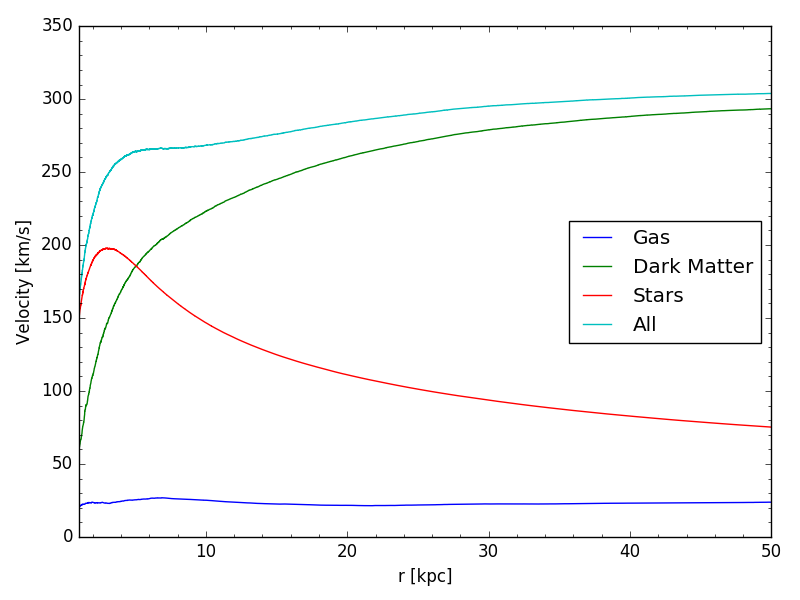
Here we use the three functions defined above to plot the rotation curve of the largest central galaxy (GroupNumber 1, SubGroupNumber 0) from the small test volume (RefL0012N0188). We find the centre (CentreOfMass_x = 12.08808994, CentreOfMass_y = 4.47437191, CentreOfMass_z 1.41333473 Mpc) using the public database.
The script loads the Coordinates and Mass for all gas, dark matter, star and black hole particles from the selected galaxy using the read_galaxy function in conjunction with the functions described above and plots the rotation curve for each component. Note that we must wrap all coordinates around the centre in order to account for the simulation’s spatial periodicity.
4.5 Plotting the temperature–density relation for a galaxy
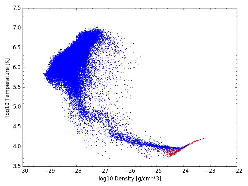
This example uses a function called read_galaxy to read the Temperature, Density and StarFormationRate for each gas particle in the largest central galaxy (GroupNumber 1, SubGroupNumber 0) from the small test volume (RefL0012N0188). It then plots Temperature vs Density with data points coloured red for a non-zero StarFormationRate and blue otherwise.
4.6 The read_eagle routine
In the previous examples we read the entire particle data from the small test volume (RefL0012N0188) and masked to only particles contained within a single galaxy. For much larger volumes, particularly the RefL0100N1504 simulation, this becomes increasingly impractical and memory intensive. For this reason, it is more manageable to read these simulations utilizing the HashTable (see Section 2.3.3 for details).
To aid with this, we provide a reading routine, named read_eagle, that reads simulation datasets efficiently using the HashTable. read_eagle is publicly available via a git repository, located at https://github.com/jchelly/read_eagle. The module must first be installed, for instructions on how to do this for Python (instructions for use with C and Fortran languages are also available) please refer to the README documentation provided within the repository.
4.6.1 read_eagle example
Below we provide an example that is a repeat of a previous example, where we create a temperature–density relation for a single galaxy, however this time using the read_eagle routine.
First, read_eagle must read information from the HashTable and Header. This is done by initializing the EagleSnapshot class with the location of any hdf5 part of the snapshot data (it does not have to be part 0). You must then select a region of interest. This is a cubic region outlined by the minimum and maximum extents in the , and directions (in cMpc/h units). For our example, we extract a 2 cMpc/h cube that is centred on the galaxy’s centre of potential (taken from the database). Datasets can then be read in a similar fashion to the examples above that did not use read_eagle, using the read_dataset routine.
Note there are additional examples within the repository, including C and Fortran examples, that explain the further functionality of read_eagle beyond simply reading datasets (for example reading files in parallel). Any queries or bugs discovered using this module can be reported via the repository.
| PartType0: Gas | ||
|---|---|---|
| Field | Equation/Par | Description |
| AExpMaximumTemperature | §3.1.1 | Expansion factor when particle had maximum temperature. |
| Coordinates | Eq. (1) | Co-moving coordinates. |
| Density | Eq. (3) | Co-moving density. |
| ElementAbundance | §3.1.2 | Mass of [Carbon, Helium, Hydrogen, Iron, Magnesium, Neon, Nitrogen, Oxygen, Silicon] divided by particle mass. |
| Entropy | §3.1.1 | Particle entropy. |
| GroupNumber | §2.3 | Friends of Friends (FoF) group number this particle belongs to in this snapshot. Values range from 1-, where is the total number of FoF groups. Values of indicate this particle does not belong to any group. |
| HostHalo_TVir_Mass | - | Estimate of host FoF group’s virial temperature, calculated from the local velocity dispersion. |
| InternalEnergy | Eq. (6) | Thermal energy per unit mass. |
| IronMassFracFromSNIa | §3.1.2 | Mass of Iron from SNIa divided by particle mass. |
| Mass | §2.3.8 | Particle mass. |
| MaximumTemperature | S3.1.1 | Maximum temperature ever reached by particle. |
| MetalMassFracFromAGB | §3.1.2 | Mass of metals received from AGB divided by particle mass. |
| MetalMassFracFromSNII | §3.1.2 | Mass of metals received from SNII divided by particle mass. |
| MetalMassFracFromSNIa | §3.1.2 | Mass of metals received from SNIa divided by particle mass. |
| Metallicity | §3.1.2 | Mass of elements heavier than Helium, including those not tracked individually, divided by particle mass |
| OnEquationOfState | §3.1.3 | 0 if particle has never been star-forming, +ve if currently star-forming, -ve if not currently star-forming. Value indicates scale factor at which it obtained its current state. Note this does not ensure the gas particle is on the equation of state for +ve values, as gas particles can yield non-zero star formation rates up to 0.5 dex above the equation of state. |
| ParticleIDs | §2.3.8 | Unique particle identifier. Index encodes the particles position in the initial conditions (see Appendix of [1] for details). |
| SmoothedElementAbundance | §3.1.2 | SPH kernel weighted ElementAbundance (see Section 2.2 of [4] for the description of kernel weighted properties in SPH). |
| SmoothedIronMassFracFromSNIa | §3.1.2 | SPH kernel weighted IronMassFracFromSNIa. |
| SmoothedMetallicity | §3.1.2 | SPH kernel weighted Metallicity. |
| SmoothingLength | §2.3.8 | Co-moving SPH smoothing kernel. |
| StarFormationRate | Eq. (11) | Instantaneous star formation rate. |
| SubGroupNumber | §2.3 | Subgroup number (as defined by subfind) this particle belongs to. Values range from 0-(-1) where is the total number of subgroups for this particular FoF group. Values of indicate this particle does not belong to any subgroup. Subgroup number 0 refers to the central subgroup, subgroup numbers greater than 0 refer to satellites. |
| Temperature | §3.1.1 | Temperature |
| TotalMassFromAGB | §3.1.2 | Total mass received from AGB. |
| TotalMassFromSNII | §3.1.2 | Total mass received from SNII. |
| TotalMassFromSNIa | §3.1.2 | Total mass received from SNIa. |
| Velocity | S2.3.8 | The peculiar velocity, (see the Appendix of [13] for more details). |
| PartType1: Dark Matter | ||
|---|---|---|
| Field | Equation/Par | Description |
| Coordinates | §2.3.8 | Co-moving coordinates. |
| GroupNumber | §2.3 | Friends of Friends (FoF) group number this particle belongs to in this snapshot. Values range from 1-, where is the total number of FoF groups. Values of indicate this particle does not belong to any group. |
| ParticleIDs | §2.3 | Unique particle identifier. Index encodes the particles position in the initial conditions (see [1] for details). |
| SubGroupNumber | §2.3 | Subgroup number (as defined by subfind) this particle belongs to. Values range from 0-(-1) where is the total number of subgroups for this particular FoF group. Values of indicate this particle does not belong to any subgroup. Subgroup number 0 refers to the central subgroup, subgroup numbers greater than 0 refer to satellites. |
| Velocity | §2.3.8 | The peculiar velocity, (see the Appendix of [13] for more details). |
| PartType4: Stars | ||
|---|---|---|
| Field | Equation/Par | Description |
| AExpMaximumTemperature | §3.1.1 | Expansion factor a when particle had highest temperature. |
| BirthDensity | §3.1.3 | Local gas density when gas particle was converted to star |
| Coordinates | §2.3.8 | Co-moving Coordinates. |
| ElementAbundance | §3.1.2 | Mass of [Carbon, Helium, Hydrogen, Iron, Magnesium, Neon, Nitrogen, Oxygen, Silicon] divided by particle mass. |
| Feedback_EnergyFraction | S3.3 | Fraction of energy used for thermal feedback, defined such that a value of unity corresponds to the energy released by the population of Type II SNe (each producing 1051 erg) described by a Chabrier IMF, with SNe progenitors having initial masses of 6-100 M⊙. |
| GroupNumber | §2.3.8 | Friends of Friends (FoF) group number this particle belongs to in this snapshot. Values range from 1-, where is the total number of FoF groups. Values of indicate this particle does not belong to any group. |
| HostHalo_TVir | - | Halo’s virial temperature. |
| HostHalo_TVir_Mass | - | Estimate of host FoF groups virial temperature, calculated from the local velocity dispersion. |
| InitialMass | §3.3 | Mass at formation time. |
| IronMassFracFromSNIa | - | Mass of Iron from SNIa divided by particle mass. |
| Mass | §3.3 | Current particle mass. |
| MaximumTemperature | §3.1.1 | Maximum temperature ever reached by particle. |
| MetalMassFracFromAGB | §3.1.2 | Mass of metals received from AGB divided by particle mass. |
| MetalMassFracFromSNII | §3.1.2 | Mass of metals received from SNII divided by particle mass. |
| MetalMassFracFromSNIa | §3.1.2 | Mass of metals received from SNIa divided by particle mass. |
| Metallicity | §3.1.2 | Mass of elements heavier than Helium, including those not tracked individually, divided by particle mass. |
| ParticleIDs | §2.3.8 | Unique particle identifier. ID is inherited from parent gas particle. |
| PreviousStellarEnrichment | §3.3 | Expansion factor when this star particle last enriched its neighbours. |
| SmoothedElementAbundance | §3.1.2 | SPH kernel weighted ElementAbundance. |
| SmoothedIronMassFracFromSNIa | §3.1.2 | SPH kernel weighted IronMassFracFromSNIa. |
| SmoothedMetallicity | §3.1.2 | SPH kernel weighted Metallicity. |
| SmoothingLength | §2.3.8 | Co-moving SPH smoothing kernel. |
| StellarEnrichmentCounter | §3.1.2 | Number of timesteps since enrichment was last performed by this particle. |
| StellarFormationTime | §3.3 | Expansion factor when this star particle was born. |
| SubGroupNumber | §2.3.8 | Subgroup number (as defined by subfind) this particle belongs to. Values range from 0-(-1) where is the total number of subgroups for this particular FoF group. Values of indicate this particle does not belong to any subgroup. Subgroup number 0 refers to the central subgroup, subgroup numbers greater than 0 refer to satellites. |
| TotalMassFromAGB | §3.1.2 | Total mass received from AGB. |
| TotalMassFromSNII | §3.1.2 | Total mass received from SNII. |
| TotalMassFromSNIa | §3.1.2 | Total mass received from SNIa. |
| Velocity | §2.3.8 | The peculiar velocity, (see the Appendix of [13] for more details). |
| PartType5: Black Holes | ||
|---|---|---|
| Field | Equation/Par | Description |
| BH_CumlAccrMass | §3.4 | Cumulative mass that has been accreted onto this black hole. |
| BH_CumlNumSeeds | §3.4 | Cumulative number of black hole seeds swallowed by this black hole. |
| BH_Density | §3.4 | Co-moving gas density at the location of the black hole. |
| BH_FormationTime | §3.4 | Scale factor when this black hole was formed. |
| BH_Mass | §3.4 | Black hole subgrid mass (see Appendix of [13] for more details). |
| BH_Mdot | §3.4 | Instantaneous black hole accretion rate. |
| BH_MostMassiveProgenitorID | §3.4 | At the time of the last BH-BH merger, this is the ParticleID of the most massive member of the pair. |
| BH_Pressure | §3.4 | Gas pressure at the location of the black hole. |
| BH_SoundSpeed | §3.4 | Gas sound speed at the location of the black hole. |
| BH_SurroundingGasVel | §3.4 | Peculiar velocity of the gas at the location of the black hole. |
| BH_TimeLastMerger | §3.4 | Expansion factor when black hole particle last accreted another black hole. 0 if the particle has never accreted another black hole. |
| Coordinates | §2.3.8 | Co-moving coordinates. |
| GroupNumber | §2.3 | Friends of Friends (FoF) group number this particle belongs to in this snapshot. Values range from 1-, where is the total number of FoF groups. Values of indicate this particle does not belong to any group. |
| HostHalo_TVir_Mass | - | Estimate of host FoF group’s virial temperature, calculated from the local velocity dispersion. |
| Mass | §2.3.8 | BH particle mass. Users should use the black hole subgrid mass (BH_Mass) for the actual black hole subgrid mass. |
| ParticleIDs | §2.3.8 | Unique particle identifier. ID is inherited from parent gas particle. |
| SmoothingLength | §2.3.8 | Co-moving SPH smoothing kernel. |
| SubGroupNumber | §2.3 | Subgroup number (as defined by subfind) this particle belongs to. Values range from 0-(-1) where is the total number of subgroups for this particular FoF group. Values of indicate this particle does not belong to any subgroup. Subgroup number 0 refers to the central subgroup, subgroup numbers greater than 0 refer to satellites. |
| Velocity | §2.3.8 | The peculiar velocity, (see the Appendix of [13] for more details). |
5 Acknowledging these data
This document is not intended to serve as a reference for eagle. Users of eagle data are kindly requested to acknowledge and cite the original sources following the instructions listed in section 4.2 of [13], which we repeat here for completeness:
To recognise the effort of the individuals involved in the design and execution of these simulations, in their post processing and in the construction of the database, we kindly request the following:
- •
- •
Publications making use of the database should add the following line in their acknowledgement section: ”We acknowledge the Virgo Consortium for making their simulation data available. The eagle simulations were performed using the DiRAC-2 facility at Durham, managed by the ICC, and the PRACE facility Curie based in France at TGCC, CEA, Bruyèresle-Châtel.”.
- •
Furthermore, publications referring to specific aspects of the subgrid models, hydrodynamics solver, or post-processing steps (such as the construction of images or photometric quantities, and the construction of merger trees), are kindly requested to not only cite the above papers, but also the original papers describing these aspects. The appropriate references can be found in section 2 of this paper and in [1].
References
- [1] J. Schaye, R. A. Crain, R. G. Bower, M. Furlong, M. Schaller, T. Theuns, C. Dalla Vecchia, C. S. Frenk, I. G. McCarthy, J. C. Helly, A. Jenkins, Y. M. Rosas-Guevara, S. D. M. White, M. Baes, C. M. Booth, P. Camps, J. F. Navarro, Y. Qu, A. Rahmati, T. Sawala, P. A. Thomas, and J. Trayford. The EAGLE project: simulating the evolution and assembly of galaxies and their environments. MNRAS, 446:521–554, January 2015.
- [2] R. A. Crain, J. Schaye, R. G. Bower, M. Furlong, M. Schaller, T. Theuns, C. Dalla Vecchia, C. S. Frenk, I. G. McCarthy, J. C. Helly, A. Jenkins, Y. M. Rosas-Guevara, S. D. M. White, and J. W. Trayford. The EAGLE simulations of galaxy formation: calibration of subgrid physics and model variations. MNRAS, 450:1937–1961, June 2015.
- [3] Planck Collaboration, P. A. R. Ade, N. Aghanim, M. I. R. Alves, C. Armitage-Caplan, M. Arnaud, M. Ashdown, F. Atrio-Barandela, J. Aumont, H. Aussel, and et al. Planck 2013 results. I. Overview of products and scientific results. A&A, 571:A1, November 2014.
- [4] V. Springel. The cosmological simulation code GADGET-2. MNRAS, 364:1105–1134, December 2005.
- [5] T. Sawala, C. S. Frenk, A. Fattahi, J. F. Navarro, R. G. Bower, R. A. Crain, C. Dalla Vecchia, M. Furlong, J. C. Helly, A. Jenkins, K. A. Oman, M. Schaller, J. Schaye, T. Theuns, J. Trayford, and S. D. M. White. The APOSTLE simulations: solutions to the Local Group’s cosmic puzzles. MNRAS, 457:1931–1943, April 2016.
- [6] A. Fattahi, J. F. Navarro, T. Sawala, C. S. Frenk, K. A. Oman, R. A. Crain, M. Furlong, M. Schaller, J. Schaye, T. Theuns, and A. Jenkins. The APOSTLE project: Local Group kinematic mass constraints and simulation candidate selection. MNRAS, 457:844–856, March 2016.
- [7] Y. M. Bahé, D. J. Barnes, C. Dalla Vecchia, S. T. Kay, S. D. M. White, I. G. McCarthy, J. Schaye, R. G. Bower, R. A. Crain, T. Theuns, A. Jenkins, S. L. McGee, M. Schaller, P. A. Thomas, and J. W. Trayford. The Hydrangea simulations: galaxy formation in and around massive clusters. ArXiv e-prints, March 2017.
- [8] D. J. Barnes, S. T. Kay, Y. M. Bahe, C. Dalla Vecchia, I. G. McCarthy, J. Schaye, R. G. Bower, A. Jenkins, P. A. Thomas, M. Schaller, R. A. Crain, T. Theuns, and S. D. M. White. The Cluster-EAGLE project: global properties of simulated clusters with resolved galaxies. ArXiv e-prints, March 2017.
- [9] M. R. Lovell, S. Bose, A. Boyarsky, R. A. Crain, C. S. Frenk, W. A. Hellwing, A. D. Ludlow, J. F. Navarro, O. Ruchayskiy, T. Sawala, M. Schaller, J. Schaye, and T. Theuns. Properties of Local Group galaxies in hydrodynamical simulations of sterile neutrino dark matter cosmologies. ArXiv e-prints, October 2016.
- [10] B. D. Oppenheimer, R. A. Crain, J. Schaye, A. Rahmati, A. J. Richings, J. W. Trayford, J. Tumlinson, R. G. Bower, M. Schaller, and T. Theuns. Bimodality of low-redshift circumgalactic O VI in non-equilibrium EAGLE zoom simulations. MNRAS, 460:2157–2179, August 2016.
- [11] K. Dolag, S. Borgani, G. Murante, and V. Springel. Substructures in hydrodynamical cluster simulations. MNRAS, 399:497–514, October 2009.
- [12] K. Dolag, S. Borgani, G. Murante, and V. Springel. Substructures in hydrodynamical cluster simulations. MNRAS, 399:497–514, October 2009.
- [13] S. McAlpine, J. C. Helly, M. Schaller, J. W. Trayford, Y. Qu, M. Furlong, R. G. Bower, R. A. Crain, J. Schaye, T. Theuns, C. Dalla Vecchia, C. S. Frenk, I. G. McCarthy, A. Jenkins, Y. Rosas-Guevara, S. D. M. White, M. Baes, P. Camps, and G. Lemson. The EAGLE simulations of galaxy formation: Public release of halo and galaxy catalogues. Astronomy and Computing, 15:72–89, April 2016.
- [14] J. W. Trayford, T. Theuns, R. G. Bower, J. Schaye, M. Furlong, M. Schaller, C. S. Frenk, R. A. Crain, C. Dalla Vecchia, and I. G. McCarthy. Colours and luminosities of z = 0.1 galaxies in the EAGLE simulation. MNRAS, 452:2879–2896, September 2015.
- [15] P. Camps, J. W. Trayford, M. Baes, T. Theuns, M. Schaller, and J. Schaye. Far-infrared and dust properties of present-day galaxies in the EAGLE simulations. MNRAS, 462:1057–1075, October 2016.
- [16] J. W. Trayford, P. Camps, T. Theuns, M. Baes, R. G. Bower, R. A. Crain, M. L. P. Gunawardhana, M. Schaller, J. Schaye, and C. S. Frenk. Optical colours and spectral indices of EAGLE galaxies with 3D dust radiative transfer code SKIRT. ArXiv e-prints, May 2017.
- [17] R. P. C. Wiersma, J. Schaye, and B. D. Smith. The effect of photoionization on the cooling rates of enriched, astrophysical plasmas. MNRAS, 393:99–107, February 2009.
- [18] P. F. Hopkins. A general class of Lagrangian smoothed particle hydrodynamics methods and implications for fluid mixing problems. MNRAS, 428:2840–2856, February 2013.
- [19] Holger Wendland. Piecewise polynomial, positive definite and compactly supported radial functions of minimal degree. Advances in Computational Mathematics, 4(1):389–396, December 1995.
- [20] R. P. C. Wiersma, J. Schaye, T. Theuns, C. Dalla Vecchia, and L. Tornatore. Chemical enrichment in cosmological, smoothed particle hydrodynamics simulations. MNRAS, 399:574–600, October 2009.
- [21] J. Schaye and C. Dalla Vecchia. On the relation between the Schmidt and Kennicutt-Schmidt star formation laws and its implications for numerical simulations. MNRAS, 383:1210–1222, January 2008.
- [22] J. Schaye. Star Formation Thresholds and Galaxy Edges: Why and Where. ApJ, 609:667–682, July 2004.
- [23] C. Dalla Vecchia and J. Schaye. Simulating galactic outflows with thermal supernova feedback. MNRAS, 426:140–158, October 2012.
- [24] V. Springel, T. Di Matteo, and L. Hernquist. Modelling feedback from stars and black holes in galaxy mergers. MNRAS, 361:776–794, August 2005.