Model reduction of controlled Fokker–Planck and Liouville–von Neumann equations

Peter Benner Address: Computational Methods in Systems and Control Theory
Max Planck Institute for Dynamics of Complex Technical Systems
Sandtorstr. 1, D-39106 Magdeburg, Germany Email address: benner@mpi-magdeburg.mpg.de , Tobias Breiten Address: Institut für Mathematik, Karl-Franzens-Universität
Heinrichstr. 36/III, A-8010 Graz, Austria Email address: tobias.breiten@uni-graz.at , Carsten Hartmann Address: Institut für Mathematik, Brandenburgische Technische Universität
Konrad-Wachsmann-Allee 1, D-03046 Cottbus, Germany Email address: carsten.hartmann@b-tu.de and Burkhard Schmidt Address: Institut für Mathematik, Freie Universität Berlin
Arnimallee 6, D-14195 Berlin, Germany Email address: burkhard.schmidt@fu-berlin.de

Date: August 24, 2026

Abstract.

Model reduction methods for bilinear control systems are compared by means of practical examples of Liouville–von Neumann and Fokker–Planck type. Methods based on balancing generalized system Gramians and on minimizing an $\mathcal{H}_{2}$ -type cost functional are considered. The focus is on the numerical implementation and a thorough comparison of the methods. Structure and stability preservation are investigated, and the competitiveness of the approaches is shown for practically relevant, large-scale examples.

Key words and phrases:

Bilinear systems, model order reduction, balanced truncation, averaging method, Hankel singular values, generalized Lyapunov equations, stochastic control.

1. Introduction

Due to the growing ability to accurately manipulate single molecules by spectroscopic techniques, numerical methods for the control of molecular systems have recently attracted a lot of attention [4, 30, 41, 61]. Key applications involve probing of mechanical properties of biomolecules by force microscopy and optical tweezers [23, 32], or the control of chemical reaction dynamics by temporally shaped femtosecond laser pulses in femtochemistry [53, 59]. A key feature of these small systems is that they are open systems, in that they are subject to noise and dissipation induced by the interaction with their environment, as a consequence of which the dynamics are inherently random and the description is on the level of probability distributions or measures rather than trajectories [47].

Depending on whether or not quantum effects play a role, the evolution of the corresponding probability distributions is governed by parabolic partial differential equations of either Liouville–von Neumann or Fokker–Planck type. The fact that the dynamics are controlled implies that the equations are bilinear as the control acts as an advection term that is coupled linearly to the probability distribution, but the main computational bottleneck clearly is that the equations, in spatially semi-discretized form, are high-dimensional which explains why model reduction is an issue; for example, in catalysis, optimal shaping of laser pulses requires the iterated integration of the dissipative Liouville–von Neumann (LvN) equation for reduced quantum mechanical density matrices, the spatial dimension of which grows quadratically with the number of quantum states involved [18]; cf. [36].

Many nonlinear control systems can be represented as bilinear systems by a suitable change of coordinates (as well as linear parametric systems), and it therefore does not come as a surprise that model reduction of bilinear control systems has recently been a field of intense research; see [7, 12] and the references therein. In recent years, various model reduction techniques that were only available for linear systems have been extended to the bilinear case, among which are Krylov subspace techniques [44, 6, 16, 39, 45], interpolation-based approaches [1, 8, 24, 25], balanced model reduction [2, 9, 49, 29], empirical POD [20, 21, 34], or $\mathcal{H}_{2}$ -optimal model reduction [8, 25, 60]. The downside of many available methods is their lack of structure preservation, most importantly, regarding asymptotic stability. In our case, positivity is an issue too, as we are dealing with probability distributions.

In this paper we compare two different model reduction techniques that represent different philosophies of model order reduction, with the focus being on practical computations and numerical tests rather than a theoretical analysis. The first approach is based on the interpolation of the Volterra series representation of the system’s transfer function and gives a local $\mathcal{H}_{2}$ -optimal approximation, because the interpolation is chosen so that the system satisfies the necessary $\mathcal{H}_{2}$ -optimality conditions upon convergence of the algorithm; see [8] for details. The second approach is based on balancing the controllable and observable subspaces, and exploits the properties of the underlying dynamical system in that it uses the properties of the controllability and observability Gramians to identify suitable small parameters that are sent to 0 to yield a reduced-order system; for details, we refer to [29]. Both methods require the solution of large-scale matrix Sylvester or Lyapunov equations. While the computational effort of balanced model reduction is essentially determined by the solution of two generalized Lyapunov equations for controllability and observability Gramians, the effort of the $\mathcal{H}_{2}$ -optimal interpolation method is mainly due to the solution of two generalized Sylvester equations in each step of the bilinear iterative rational Krylov algorithm (B-IRKA). We stress that both generalized Lyapunov or Sylvester equations can be solved iteratively at comparable numerical cost (for a given accuracy), but they all require the dynamics of the uncontrolled system to be asymptotically stable [55]. However, as both the dissipative LvN and Fokker-Planck operators have a simple eigenvalue zero, stability has to be enforced before solving Lyapunov or Sylvester equations, and in this paper we systematically compared stabilization techniques for both approaches.

The outline of the article is as follows: In Section 2 we briefly discuss the basic properties of bilinear systems and set the notation for the remainder of the article. Model reduction by $\mathcal{H}_{2}$ -norm minimization and balancing are reviewed in Sections 3 and 4, along with some details regarding the numerical implementation for the specific applications considered in this paper in Section 5. Finally, in Section 6 we study model reduction of the Fokker-Planck equation comparing balancing and $\mathcal{H}_{2}$ -norm minimization, and in Section 7 we carry out a similar study for the dissipative Liouville–von Neumann equation. We discuss our observations in Section 8. The article contains an appendix, Appendix A, that records some technical lemmas related to the asymptotic stability of bilinear systems.

2. Bilinear control systems

We start by setting the notation that will be used throughout this article. Let $x(t)\in{\mathbb{C}}^{n}$ be governed by the time-inhomogeneous differential equation

(2.1)

\frac{\,\mathrm{d}x}{\,\mathrm{d}t}=Ax+\sum_{k=1}^{m}\left(N_{k}x+b_{k}\right)u_{k}\,,\quad x(0)=x_{0}\,,

with coefficients $A,N_{k}\in{\mathbb{C}}^{n\times n}$ , $b_{k}\in{\mathbb{C}}^{n}$ and $u=(u_{1},\ldots,u_{m})^{T}$ being a vector of bounded measurable controls $u_{i}(t)\in U\subset{\mathbb{C}}$ . We assume that not all state variables $x$ are relevant or observable, so we augment (2.1) by a linear output equation

(2.2)

y=Cx\,,

with $C\in{\mathbb{C}}^{l\times n}$ , $l\leq n$ . The systems of equations (2.1)–(2.2) is called a bilinear control system with inputs $u(t)\in U^{m}\subset{\mathbb{C}}^{m}$ and outputs $y(t)\in{\mathbb{C}}^{l}$ .

As is well-known, see e.g. [48, 60], an explicit output representation for (2.2) can be obtained by means of successive approximations. The resulting so-called Volterra series is given as

(2.3)		$\displaystyle y(t)$	$\displaystyle=\sum_{k=1}^{\infty}\int_{0}^{\infty}\cdots\int_{0}^{\infty}\sum_{\ell_{1},\dots,\ell_{k}=1}^{m}Ce^{As_{k}}N_{\ell_{1}}e^{As_{k-1}}N_{\ell_{2}}\cdots e^{As_{2}}N_{\ell_{k-1}}e^{As_{1}}b_{\ell_{k}}$
(2.3)			$\displaystyle\times u_{\ell_{1}}(t-s_{k})u_{\ell_{2}}(t-s_{k}-s_{k-1})\cdots u_{\ell_{k}}(t-\sum_{j=1}^{k}s_{j})\,\,\mathrm{d}s_{1}\cdots\,\mathrm{d}s_{k}.$

Moreover, based on a multivariate Laplace transform of these integrands, the system can alternatively be analyzed in a generalized frequency domain by means of generalized transfer functions. Since this will not be essential for the results presented here, we refrain from a more detailed discussion and refer to, e.g., [48].

2.1. Reduced-order models

We seek coefficients $\hat{A},\hat{N}_{k}\in{\mathbb{C}}^{d\times d}$ , $\hat{b}_{k}\in{\mathbb{C}}^{d}$ and $\hat{C}\in{\mathbb{C}}^{l\times d}$ with $d\ll n$ such that

(2.4)		$\displaystyle\frac{\,\mathrm{d}\xi}{\,\mathrm{d}t}$	$\displaystyle=\hat{A}\xi+\sum_{k=1}^{m}\left(\hat{N}_{k}\xi+\hat{b}_{k}\right)u_{k}\,,\quad\xi(0)=\xi_{0}\,,$
(2.4)		$\displaystyle\hat{y}$	$\displaystyle=\hat{C}\xi$

has an input-output behavior that is similar to (2.1)–(2.2). In other words, we seek a reduced-order model with the property that for any admissible control input $u$ (to be defined below), the error in the output signal,

(2.5)

\delta(t)=\|\hat{y}(t)-y(t)\|\,,

is small, relative to $\|u\|$ (in some norm) and uniformly on bounded time intervals.

As will be outlined below, both model reduction schemes considered in this paper are closely related to the solutions of the following adjoint pair of generalized Lyapunov equations:

(2.6)

AP+PA^{*}+\sum_{k=1}^{m}N_{k}PN_{k}^{*}+BB^{*}=0\,

and

(2.7)

A^{*}Q+QA+\sum_{k=1}^{m}N^{*}_{k}QN_{k}+C^{*}C=0\,,

where, in the first equation, we have introduced the shorthand $B=(b_{1},\ldots,b_{m})\in{\mathbb{C}}^{n\times m}$ . The Hermitian and positive semi-definite matrices $P,Q\in{\mathbb{C}}^{n\times n}$ are called the controllability and observability Gramians associated with (2.1)–(2.2)—assuming well-posedness of the Lyapunov equations and hence existence and uniqueness of $P$ and $Q$ . The relevance of the Gramians for model reduction is related to the fact that the nullspace of the controllability Gramian contains only states that cannot be reached by any bounded measurable control and that the system will not produce any output signal, if the dynamics is initialized in the nullspace of the observability Gramian [33]; as a consequence one can eliminate states that belong to $\ker(P)\cap\ker(Q)$ without affecting the input-output behavior of (2.1)–(2.2); cf. [2].

2.2. Standing assumptions

The following assumptions will be used throughout to guarantee existence and uniqueness of the solutions to the generalized Lyapunov equations (Assumption 1) and existence and uniqueness of the solution of the bilinear system (2.1) for all $t\geq 0$ (Assumptions 2 and 3):

Assumption 1: There exists constants $\lambda,\mu>0$ , such that

\|\exp(At)\|\leq\lambda\exp(-\mu t)

and

\frac{\lambda^{2}}{2\mu}\sum_{k=1}^{m}\|N_{k}\|^{2}<1\,,

where $\|\cdot\|=\|\cdot\|_{2}$ is the matrix 2-norm that is induced by the Euclidean norm $|\cdot|$ .

Assumption 2: The bilinear system (2.1)–(2.2) is bounded-input-bounded-output (BIBO) stable, i.e., there exists $M<\infty$ , such that for any input $u$ with

\|u\|_{\infty}=\sup_{t\in[0,\infty)}|u(t)|\leq M

the output $y(t)$ is uniformly bounded.

Assumption 3: The admissible controls $u\colon[0,\infty)\to U^{m}\subset{\mathbb{C}}^{m}$ are continuous, bounded and square integrable, i.e., $u\in{\mathcal{C}}_{b}([0,\infty),U^{m})$ with

\|u\|_{2}=\left(\int_{0}^{\infty}|u(t)|^{2}\,\,\mathrm{d}t\right)^{1/2}<\infty.

Specifically, we require that the admissible controls are uniformly bounded by

M<\frac{\mu}{\lambda}\sum_{k=1}^{m}\|N_{k}\|\,,

with $\lambda,\mu$ as in Assumption 1, which by BIBO stability (Assumptions 2) implies that the output $y(t)$ is bounded for all $t\geq 0$ (cf. [52]).

3. $\mathcal{H}_{2}$ optimal model reduction of bilinear systems

In this section, we recall some existing results on $\mathcal{H}_{2}$ -optimal model order reduction for bilinear systems. For a more detailed presentation, see [60, 8, 24].

For a better understanding of the subsequent concepts, let us briefly focus on the linear case, i.e., $N_{k}=0$ in (2.1). Here, the Volterra series representation (2.3) simplifies to $y(t)=\int_{0}^{\infty}Ce^{As}Bu(t-s)\,\mathrm{d}s.$ If the input signal is a Dirac mass at $0,$ we obtain the impulse response $h(t)=Ce^{At}B.$ The $\mathcal{H}_{2}$ -norm for linear systems now is simply defined as the $L_{2}$ -norm of the impulse response, i.e.,

\displaystyle\|h\|_{L^{2}(0,\infty;{\mathbb{C}}^{m})}^{2}=\int_{0}^{\infty}\mathrm{tr}(B^{*}e^{A^{*}t}C^{*}Ce^{At}B)\,\mathrm{d}t.

Based on the latter definition and the Volterra series, in [60], the $\mathcal{H}_{2}$ -norm has been generalized for bilinear systems as follows.

Definition 3.1.

Let $\Sigma=(A,N_{1},\dots,N_{k},B,C)$ denote a bilinear system as in (2.1). We then define its $\mathcal{H}_{2}$ -norm by

\|\Sigma\|_{\mathcal{H}_{2}}^{2}=\mathrm{tr}\left(\sum_{k=1}^{\infty}\int_{0}^{\infty}\cdots\int_{0}^{\infty}\sum_{\ell_{1},\dots,\ell_{k}=1}^{m}g_{k}^{(\ell_{1},\dots,\ell_{k})}(g_{k}^{(\ell_{1},\dots,\ell_{k})})^{*}\,\mathrm{d}s_{1}\cdots\,\mathrm{d}s_{k}\right),

with $g_{k}^{(\ell_{1},\dots,\ell_{k})}(s_{1},\dots,s_{k})=Ce^{As_{k}}N_{\ell_{1}}e^{As_{k-1}}N_{\ell_{2}}\cdots e^{As_{1}}b_{\ell_{k}}.$

Obviously, for a bilinear system having a finite $\mathcal{H}_{2}$ -norm, it is required that the system is stable in the linear sense, i.e., $A$ has only eigenvalues in ${\mathbb{C}}_{-}.$ Moreover, the matrices $N_{k}$ have to be sufficiently bounded. From [60], let us recall that Assumption 1 ensures that the bilinear system under consideration has a finite $\mathcal{H}_{2}$ -norm, which, moreover, can be computed by means of the solution $P$ and $Q$ of the generalized Lyapunov equations (2.6) and (2.7), respectively. In particular, we have that

\displaystyle\|\Sigma\|_{\mathcal{H}_{2}}^{2}=\mathrm{tr}(CPC^{*})=\mathrm{tr}(B^{*}QB).

Given a fixed system dimension $l$ the goal of $\mathcal{H}_{2}$ -optimal model order reduction now is to construct a reduced-order bilinear system $\tilde{\Sigma}$ such that

\|\Sigma-\tilde{\Sigma}\|_{\mathcal{H}_{2}}=\min_{\begin{subarray}{c}\dim(\hat{\Sigma})\ =\ l\ \\ \hat{\Sigma}\text{ stable}\end{subarray}}\|\Sigma-\tilde{\Sigma}\|_{\mathcal{H}_{2}}.

Unfortunately, already in the linear case this is a highly nonconvex minimization problem such that finding a global minimizer is out of reach. Instead, we aim at constructing $\tilde{\Sigma}$ such that first-order necessary conditions for $\mathcal{H}_{2}$ -optimality are fulfilled. In [60], the optimality conditions from [58] are extended to the bilinear case. More precisely, it is shown that an $\mathcal{H}_{2}$ -optimal reduced-order model is defined by a Petrov-Galerkin projection of the original model. Given a reduced-order system $\hat{\Sigma},$ let us consider the associated error system

(3.1)

\begin{aligned} A_{e}=\begin{bmatrix}A&0\\ 0&\hat{A}\end{bmatrix},\quad\end{aligned}\begin{aligned} N_{k,e}=\begin{bmatrix}N_{k}&0\\ 0&\hat{N}_{k}\end{bmatrix},\quad\end{aligned}\begin{aligned} B_{e}=\begin{bmatrix}B\\ \hat{B}\end{bmatrix},\quad\end{aligned}\begin{aligned} C_{e}=\begin{bmatrix}C&-\hat{C}\end{bmatrix},\end{aligned}

as well as the generalized Lyapunov equations associated with it

(3.2)		$\displaystyle A_{e}P_{e}+P_{e}A_{e}^{}+\sum_{k=1}^{m}N_{k,e}P_{e}N_{k,e}^{}+B_{e}B_{e}^{*}$	$\displaystyle=0,$
(3.2)		$\displaystyle A_{e}^{}Q_{e}+Q_{e}A_{e}+\sum_{k=1}^{m}N_{k,e}^{}Q_{e}N_{k,e}+C_{e}^{*}C_{e}$	$\displaystyle=0.$

Assuming the partitioning

(3.3)

P_{e}=\begin{bmatrix}P&X\\ X^{*}&\hat{P}\end{bmatrix},\quad Q_{e}=\begin{bmatrix}Q&Y\\ Y^{*}&\hat{Q}\end{bmatrix},

the first-order necessary optimality conditions now are

(3.4)		$\displaystyle Y^{}AX+\hat{Q}^{}\hat{A}\hat{P}$	$\displaystyle=0,$		$\displaystyle Y^{}N_{k}X+\hat{Q}^{}\hat{N}_{k}\hat{P}$	$\displaystyle=0,$
(3.4)		$\displaystyle Y^{}B+\hat{Q}^{}\hat{B}$	$\displaystyle=0,$		$\displaystyle CX-\hat{C}\hat{P}$	$\displaystyle=0.$

In [60] the authors have proposed a gradient flow technique to construct a reduced-order model satisfying (3.4). Since here we are interested in computations for large-scale systems for which this technique is not feasible, we instead use the iterative method from [8]. The main idea is inspired by the iterative rational Krylov algorithm from [28] and relies on solving generalized Sylvester equations of the form

	$\displaystyle AX+X\hat{A}^{}+\sum_{k=1}^{m}N_{k}X\hat{N}_{k}^{}+B\hat{B}^{*}$	$\displaystyle=0,$
	$\displaystyle A^{}Y+Y\hat{A}+\sum_{k=1}^{m}N_{k}^{}Y\hat{N}_{k}-C^{*}\hat{C}$	$\displaystyle=0.$

Based on a given reduced-order model $(\hat{A}_{i},\hat{N}_{k,i},\hat{B}_{i},\hat{C}_{i})$ , the subspaces spanned by columns of the solutions $X_{i},Y_{i}\in{\mathbb{C}}^{n\times l}$ are used to generate an updated reduced-order model. More precisely, given unitary matrices $V_{i},W_{i}\in\mathbb{C}^{n\times l}$ such that $\mathrm{span}(V_{i})=\mathrm{span}(X_{i})$ and $\mathrm{span}(W_{i})=\mathrm{span}(Y_{i}),$ we set

	$\displaystyle\hat{A}_{i+1}$	$\displaystyle=(W_{i}^{}V_{i})^{-1}W_{i}^{}AV_{i},\ \ \hat{N}_{i+1}=(W_{i}^{}V_{i})^{-1}W_{i}^{}N_{k}V_{i},$
	$\displaystyle\hat{B}_{i+1}$	$\displaystyle=(W_{i}^{}V_{i})^{-1}W_{i}^{}B,\ \ \hat{C}_{i+1}=CV_{i}.$

This type of fixed-point iteration is repeated until the reduced-order model is numerically converged up to a prescribed tolerance. For more details on the iteration, we also refer to [8].

4. Balanced model reduction for bilinear systems

We shall briefly explain model reduction based on balancing controllability and observability. To this end we assume that the generalized Gramian matrices $P,Q$ are both Hermitian positive definite which is guaranteed by the assumption that the bilinear system (2.1)–(2.2) is completely controllable and observable:

Assumption 4: The matrix pair $(A,B)$ is controllable, i.e.,

{\rm rank}(B\,AB\,A^{2}B\ldots A^{n-1}B)=n\,.

Assumption 5: The matrix pair $(A,C)$ is observable, i.e.,

{\rm rank}(C^{*}\,A^{*}C^{*}\,A^{2}C^{*}\ldots A^{n-1}C^{*})=n\,.

4.1. Singularly perturbed bilinear systems

We consider a balancing transformation $x\mapsto T^{-1}x$ under which the Gramians transform according to [42]

(4.1)

T^{-1}Q\left(T^{-1}\right)^{*}=\Sigma=T^{*}PT\,,

where the diagonal matrix $\Sigma={\rm diag}(\sigma_{1},\sigma_{2},\ldots,\sigma_{n})$ with $\sigma_{1}\geq\sigma_{2}\geq\ldots\geq\sigma_{n}>0$ contains the real-valued Hankel singular values (HSV) of the system. Under the linear map $T$ , the coefficients of (2.1)–(2.2) transform according to

(4.2)

(A,N_{k},B,C)\mapsto(T^{-1}AT,\,T^{-1}N_{k}T,\,T^{-1}B,\,CT)\,,\quad k=1,\ldots,m\,.

As the Hankel singular values are the square roots of the eigenvalues of the product $QP$ , they are independent of the choice of coordinates. It can be shown (e.g. [5]) that a balancing transformation that makes the two Gramians $Q$ and $P$ equal and diagonal is given by the matrix $T=\Sigma^{-\frac{1}{2}}V^{T}R$ with inverse $T^{-1}=S^{T}U\Sigma^{-1/2}$ where the matrices $U,V,S,R$ are defined by the Cholesky decompositions $P=S^{T}S$ and $Q=R^{T}R$ of the two Gramians solving (2.6) and (2.7), and their singular value decomposition $SR^{T}=U\Sigma V^{T}$ .

Now suppose that $\Sigma=(\Sigma_{1},\Sigma_{2})$ with $\Sigma_{1}\in{\mathbb{R}}^{d\times d}$ and $\Sigma_{2}\in{\mathbb{R}}^{(n-d)\times(n-d)}$ corresponding to the splitting of the system states into relevant and irrelevant states. Further assume that $\Sigma_{2}\ll\Sigma_{1}$ in the sense that the smallest entry of $\Sigma_{1}$ is much larger than the largest entry of $\Sigma_{2}$ . The rationale of balanced model reduction is based on a continuity argument: if the space of the uncontrollable and unobservable states is spanned by the singular vectors corresponding to $\Sigma_{2}=0$ , then, by continuity of the solution of (2.1)–(2.2) on the system’s coefficients, small singular values should indicate hardly controllable and observable states that do not contribute much to the input-output behavior of the system.

Using the notation $\Sigma_{2}={\mathcal{O}}(\epsilon)$ with $0<\epsilon\ll 1$ and partitioning the balanced coefficients according to the splitting into large and small HSV, then yields the following singularly perturbed system of equations (see [29, 31]):

(4.3)

\begin{split}\frac{\,\mathrm{d}z^{\epsilon}_{1}}{\,\mathrm{d}t}&=\tilde{A}_{11}z^{\epsilon}_{1}+\frac{1}{\sqrt{\epsilon}}\tilde{A}_{12}z^{\epsilon}_{2}+\sum_{k=1}^{m}\left(\tilde{N}_{k,11}z^{\epsilon}_{1}+\frac{1}{\sqrt{\epsilon}}\tilde{N}_{k,12}z^{\epsilon}_{2}+\tilde{b}_{k,1}\right)u_{k}\\ \sqrt{\epsilon}\frac{\,\mathrm{d}z^{\epsilon}_{2}}{\,\mathrm{d}t}&=\tilde{A}_{21}z^{\epsilon}_{1}+\frac{1}{\sqrt{\epsilon}}\tilde{A}_{22}z^{\epsilon}_{2}+\sum_{k=1}^{m}\left(\tilde{N}_{k,21}z^{\epsilon}_{1}+\frac{1}{\sqrt{\epsilon}}\tilde{N}_{k,22}z^{\epsilon}_{2}+\tilde{b}_{k,2}\right)u_{k}\\ y^{\epsilon}&=\tilde{C}_{1}z^{\epsilon}_{1}+\frac{1}{\sqrt{\epsilon}}\tilde{C}_{2}z^{\epsilon}_{2}\,\end{split}

Here $z=T^{-1}x$ , with $z=(z_{1},z_{2})\in{\mathbb{C}}^{d}\times{\mathbb{C}}^{n-d}$ , denotes the balanced state vector where the splitting into $z_{1}$ , $z_{2}$ is in accordance with the splitting of the HSV into $\Sigma_{1}$ and $\Sigma_{2}$ . The splitting of the balanced coefficients

(4.4)

\tilde{A}=T^{-1}AT,\,\tilde{N}_{k}=T^{-1}N_{k}T,\,\tilde{b}_{k}=T^{-1}b_{k},\,\tilde{C}=CT\,

into $\tilde{A}_{11}$ , $\tilde{A}_{12}$ etc. can be understood accordingly.

4.2. An averaging principle for bilinear systems

In order to derive reduced-order models of (2.1)–(2.2), we consider the limit $\epsilon\to 0$ in (4.3). This amounts to the limit of vanishing small HSV $\Sigma_{2}$ in the original bilinear system.

We suppose that Assumptions 1–5 hold for all $\epsilon>0$ . As we will show in Appendix A, the results in [11] can be modified to show that the matrices $\tilde{A}_{11}$ and $\tilde{A}_{22}$ are Hurwitz, and that their eigenvalues are bounded away from the imaginary axis. In this case, BIBO stability of the system together with the assumptions on the admissible controls imply that $z^{\epsilon}_{2}\to 0$ pointwise for all $t>0$ as $\epsilon\to 0$ . However, the rate at which $z^{\epsilon}_{2}$ tends to zero and hence the limiting bilinear systems clearly depends on the controls $u$ , especially when $u$ depends on $\epsilon$ . We give only a formal justification of the different candidate equations that can be obtained in the limit of vanishing small HSV and refer to [29] for further details.

4.3. Balanced truncation

If $z^{\epsilon}_{2}=o(\sqrt{\epsilon})$ , we expect that the first two equations in (4.3) decouple as $\epsilon\to 0$ , which implies that the limiting bilinear system will be of the form

(4.5)

\begin{split}\frac{\,\mathrm{d}z_{1}}{\,\mathrm{d}t}&=\tilde{A}_{11}z_{1}+\sum_{k=1}^{m}\left(\tilde{N}_{k,11}z_{1}+\tilde{b}_{k,1}\right)u_{k}\\ y&=\tilde{C}_{1}z_{1}\,.\end{split}

The assumption that $z^{\epsilon}_{2}$ goes to zero faster than $\sqrt{\epsilon}$ is the basis of the traditional balanced truncation approach in which the weakly controllable and observable degrees of freedom are eliminated by projecting the equations to the linear subspace

S_{1}=\{(z_{1},z_{2})\in{\mathbb{C}}^{n}\colon z_{2}=0\}\simeq{\mathbb{C}}^{d}.

The validity of the approximation for all $t\geq 0$ requires that $z_{2}^{\epsilon}(0)=0$ ; cf. Remark 4.2 below.

4.4. Singular perturbation

If $z^{\epsilon}_{2}={\mathcal{O}}(\sqrt{\epsilon})$ the $z_{1}$ , $z_{2}$ equations do not decouple as $\epsilon\to 0$ , and the limiting equation turns out to be different from (4.5). To reveal it, it is convenient to introduce scaled variables by $z_{2}=\sqrt{\epsilon}\zeta$ by which (4.3) becomes

(4.6)

\begin{split}\frac{\,\mathrm{d}z^{\epsilon}_{1}}{\,\mathrm{d}t}&=\tilde{A}_{11}z^{\epsilon}_{1}+\tilde{A}_{12}\zeta^{\epsilon}+\sum_{k=1}^{m}\left(\tilde{N}_{k,11}z^{\epsilon}_{1}+\tilde{N}_{k,12}\zeta^{\epsilon}+\tilde{b}_{k,1}\right)u_{k}\\ \epsilon\frac{\,\mathrm{d}\zeta^{\epsilon}}{\,\mathrm{d}t}&=\tilde{A}_{21}z^{\epsilon}_{1}+\tilde{A}_{22}\zeta^{\epsilon}+\sum_{k=1}^{m}\left(\tilde{N}_{k,21}z^{\epsilon}_{1}+\tilde{N}_{k,22}\zeta^{\epsilon}+\tilde{b}_{k,2}\right)u_{k}\\ y^{\epsilon}&=\tilde{C}_{1}z^{\epsilon}_{1}+\tilde{C}_{2}\zeta^{\epsilon}\,.\end{split}

Equation (4.6) is an instance of a slow-fast system with $z_{1}$ being the slow variable and $\zeta=z_{2}/\sqrt{\epsilon}$ being fast, and for non-pathological controls $u$ , the averaging principle applies [27]. The idea of the averaging principle is to average the fast variables in the equation for $z_{1}$ against their invariant measure, because whenever $\epsilon$ is sufficiently small, the fast variables relax to their invariant measure while the slow variables are effectively frozen, and therefore the slow dynamics move under the average influence of the fast variables. This clearly requires that the convergence of the fast dynamics is sufficiently fast and independent of the initial conditions. The auxiliary fast subsystem for frozen slow variable $z_{1}$ reads

(4.7)

\frac{\,\mathrm{d}\tilde{\zeta}}{\,\mathrm{d}\tau}=\tilde{A}_{22}\left(\tilde{\zeta}+\tilde{A}_{22}^{-1}\tilde{A}_{21}z_{1}\right)+\sum_{k=1}^{m}\left(\tilde{N}_{k,22}\left(\tilde{\zeta}+\tilde{A}_{22}^{-1}\tilde{A}_{21}z_{1}\right)+\tilde{B}_{k,2}\right)\tilde{u}_{k}\,,

with

(4.8)

\tilde{B}_{k,2}=\left(\tilde{N}_{k,21}-\tilde{N}_{k,22}\tilde{A}_{22}^{-1}\tilde{A}_{21}z_{1}\right)+\tilde{b}_{k,2}\,.

It is obtained from (4.6) by rescaling the equations according to $\tau=t/\epsilon$ and $\tilde{\zeta}(\tau)=\zeta^{\epsilon}(\epsilon\tau)$ , $\tilde{u}(\tau)=u(\epsilon\tau)$ and sending $\epsilon\to 0$ . Since the admissible controls decay on time scales that are of order one in $t$ (i.e. ${\mathcal{O}}(1/\epsilon)$ in $\tau$ ), it follows that

\lim_{\tau\to\infty}\tilde{\zeta}(\tau;z_{1})=-\tilde{A}_{22}^{-1}\tilde{A}_{21}z_{1}\,.

In other words, for fixed $z_{1}$ the fast dynamics converge to the Dirac mass $\delta_{m}$ at $m=-\tilde{A}_{22}^{-1}\tilde{A}_{21}z_{1}$ . This can be rephrased by saying that for all admissible controls and in the limit $\epsilon\to 0$ the dynamics (4.6) collapse to the invariant subspace

S_{2}=\{(z_{1},z_{2})\in{\mathbb{C}}^{n}\colon z_{2}=-\tilde{A}_{22}^{-1}\tilde{A}_{21}z_{1}\}\simeq{\mathbb{C}}^{d}.

Averaging the fast variables in (4.6) against their invariant measure $\delta_{m}$ , then yields the averaged equation for the slow variables:

(4.9)

\displaystyle\begin{aligned} \frac{\,\mathrm{d}z_{1}}{\,\mathrm{d}t}&=\hat{A}z_{1}+\sum_{k=1}^{m}\left(\hat{N}_{k}z_{1}+\tilde{b}_{1,k}\right)u_{k}\\ y&=\hat{C}z_{1}\,,\end{aligned}

with the coefficients

(4.10)	$\displaystyle\hat{A}$	$\displaystyle=\tilde{A}_{11}-\tilde{A}_{12}\tilde{A}_{22}^{-1}\tilde{A}_{21}$
	$\displaystyle\hat{N}_{k}$	$\displaystyle=\tilde{N}_{k,11}-\tilde{N}_{k,12}\tilde{A}_{22}^{-1}\tilde{A}_{21}$
	$\displaystyle\hat{C}$	$\displaystyle=\tilde{C}_{1}-\tilde{C}_{2}\tilde{A}_{22}^{-1}\tilde{A}_{21}\,.$

The situation here is special, in that the controls decay sufficiently fast so that the invariant measure of the fast variables is independent of $u$ . For other choices of admissible controls, however, the invariant measure may depend on $u$ , which then gives rise to averaged equations with measure-valued right hand side [26, 27, 54]. The following approximation result has been proved in [29]; cf. [56].

Theorem 4.1.

Let $u=u^{\epsilon,\gamma}$ in (4.6) be admissible, satisfying $u(t)=u(t/\epsilon^{\gamma})$ for some $0<\gamma<1$ . Further let $y^{\epsilon}(t)$ be the observed solution of (4.6) with consistent initial conditions $(z_{1}^{\epsilon}(0),\zeta^{\epsilon}(0))=(\eta,-\tilde{A}_{22}^{-1}\tilde{A}_{21}\eta)$ , and let $\bar{y}(t)$ denote the output of the averaged equation (4.9) on the bounded time interval $[0,T]$ , starting from the same $z_{1}(0)=\eta$ . Then there exists a constant $C=C(T)$ , such that

\sup_{0\leq t\leq T}\left|y^{\epsilon}(t)-\hat{y}(t)\right|\leq C\epsilon^{\gamma}\,.

We should stress that it is possible to relax the condition on the initial conditions that guarantees that $(z_{1}^{\epsilon}(0),\zeta^{\epsilon}(0))\in S_{2}$ . In this case there will be a transient initial layer of thickness ${\mathcal{O}}(\sqrt{\epsilon})$ , in which there is a rapid adjustment of the initial conditions to the invariant subspace $S_{2}$ and during which the averaged dynamics deviates from the original dynamics, with an ${\mathcal{O}}(1)$ error. A uniform approximation on $[0,T]$ can then be obtained by a so called matched asymptotic expansion that matches an initial layer approximation with the averaged dynamics [43].

Remark 4.2.

For single-input systems ( $m=1$ ), a sufficient condition for BIBO stability of (2.1) is that $A$ is Hurwitz, in which case there exists a $\delta>0$ , such that $A+sN$ is Hurwitz for all $s\in[-\delta,\delta]$ . The stability of $A$ is inherited by the Schur complement $\hat{A}$ , in (4.9) and consequently $\hat{A}+s\hat{N}$ inherits stability, with a possibly smaller stability region. (See Appendix A for details.) Hence reduced single-input systems are again BIBO stable.

5. Numerical details

Before testing $\mathcal{H}_{2}$ and balanced model reduction for examples from stochastic control and quantum dynamics, see Secs. 6 and 7, respectively, we will first focus on the numerical issues related to the scaling of the controls and the preprocessing of the unstable $A$ matrix.

5.1. Structured bilinear systems

The subsequent numerical examples share several special properties that result from a physical interpretation and that require a careful numerical treatment. In this section, we provide some insight in how the model reduction methods are applied to the particularly structured bilinear systems. In fact, in the FPE as well as in the LvNE context, the initial setup leads to a purely bilinear system of the form

(5.1)		$\displaystyle\dot{x}(t)$	$\displaystyle=Ax(t)+\sum_{k=1}^{m}N_{k}x(t)u_{k}(t),\quad x(0)=x_{0},$
(5.1)		$\displaystyle y(t)$	$\displaystyle=Cx(t).$

In either case, the system exhibits a nontrivial stationary solution $x_{e}$ corresponding to a simple eigenvalue $0$ of the system matrix $A,$ i.e., $Ax_{e}=0.$ For the applications we are interested in the deviation of the state $x$ from the stationary solution. Let us therefore introduce the reference state $\tilde{x}=x-x_{e}$ that is governed by the bilinear system

(5.2)		$\displaystyle\dot{\tilde{x}}(t)$	$\displaystyle=A\tilde{x}(t)+\sum_{k=1}^{m}N_{k}\tilde{x}(t)u_{k}(t)+\underbrace{\begin{bmatrix}N_{1}x_{e},\dots,N_{k}x_{e}\end{bmatrix}}_{B}u(t),\quad\tilde{x}(0)=x_{0}-x_{e},$
(5.2)		$\displaystyle y(t)$	$\displaystyle=C\tilde{x}(t)+Cx_{e},$

where the term $Cx_{e}$ can be interpreted as a constant nonzero feedthrough $D$ of the system. For the reduced-order model, we thus may simply set $\hat{D}=Cx_{e}$ such that we can simply focus on the output operator $C.$ In accordance with standard model reduction concepts that assume a homogeneous initial condition, here we assume that the initial state of the original system is the equilibrium, i.e., $\tilde{x}(0)=x_{e}-x_{e}=0.$ While the system now has been transformed from a purely bilinear into a standard bilinear system, we still have to deal with the problem of a system matrix that is not asymptotically stable. In what follows, we present two different techniques that bypass this problem.

5.2. Sparsity preserving projection

In our examples, the system matrices are mass and positivity preserving. Numerically this is reflected in the fact that the system matrix $A$ as well as the bilinear coupling matrices have zero row sum. In other words, the vector $\mathbf{1}_{n}:=\begin{bmatrix}1,\dots,1\end{bmatrix}^{*}\in{\mathbb{C}}^{n}$ satisfies $\mathbf{1}_{n}^{*}A=\mathbf{1}_{n}^{*}N_{k}=0.$ The intuitive idea now is splitting the state into the direct sum of the asymptotically stable subspace and the eigenspace associated with the eigenvalue $0.$ Since a straightforward implementation in general will destroy the sparsity pattern of the matrices, we suggest to use a particular decomposition that has been introduced in a similar setup in [17]. Define the matrix

\displaystyle R=\begin{bmatrix}I&0\\ 0&0\end{bmatrix}+x_{e}e_{n}^{*}-e_{n}\begin{bmatrix}\mathbf{1}_{n-1}^{*}&0\end{bmatrix},

where $e_{n}$ denotes the $n$ -th unit vector in ${\mathbb{C}}^{n}.$ An easy calculation now shows that the inverse $R^{-1}$ is given as

\displaystyle R^{-1}=\begin{bmatrix}I&0\\ 0&0\end{bmatrix}+e_{n}\mathbf{1}^{*}-\begin{bmatrix}\tilde{x}_{e}\\ 0\end{bmatrix}\mathbf{1}^{*},

where the vector $\tilde{x}_{e}\in{\mathbb{C}}^{n-1}$ consists of the first $n-1$ components of $x_{e}\in{\mathbb{C}}^{n}.$ Assume that the matrices $A,N_{k}$ and $B$ are partitioned as follows

\displaystyle A=\begin{bmatrix}\tilde{A}&A_{(1:n-1,n)}\\ *&*\end{bmatrix},\ \ N_{k}=\begin{bmatrix}\tilde{N}_{k}&N_{k,(1:n-1,n)}\\ *&*\end{bmatrix},\ \ B=\begin{bmatrix}\tilde{B}\\ *\end{bmatrix},

with $\tilde{A},\tilde{N}_{k}\in{\mathbb{C}}^{n-1\times n-1}$ and $\tilde{B}\in{\mathbb{C}}^{n-1\times m}.$ Finally, a state space transformation $z:=R^{-1}\tilde{x}$ yields the equivalent bilinear system

(5.3)		$\displaystyle\dot{z}(t)$	$\displaystyle=(R^{-1}AR)z(t)+\sum_{k=1}^{m}(R^{-1}N_{k}R)z(t)u_{k}(t)+(R^{-1}B)u(t),\quad z(0)=0,$
(5.3)		$\displaystyle y(t)$	$\displaystyle=(CR)z(t)+Cx_{e}.$

Making use of the relations $Ax_{e}=0=A^{*}\mathbf{1}_{n}=N_{k}^{*}\mathbf{1}_{n},$ we conclude that the last row of $R^{-1}AR,R^{-1}N_{k}R$ and $R^{-1}B=R^{-1}N_{k}x_{e}$ is zero. This implies that the last component of $z(t)$ is constant, and, due to $z(0)=0$ vanishes for all times $t.$ As a consequence, we can focus on the first $n-1$ components $\tilde{z}(t)$ of $z(t)$ which, after some calculations, can be shown to satisfy

	$\displaystyle\tilde{z}(t)$	$\displaystyle=(\tilde{A}-A_{(1:n-1,n)}\mathbf{1}_{n-1}^{})\tilde{z}(t)+\sum_{k=1}^{m}(\tilde{N}_{k}-N_{k,(1:n-1,n)}\mathbf{1}_{n-1}^{})\tilde{z}(t)u_{k}(t)+\tilde{B}u(t),$
	$\displaystyle y(t)$	$\displaystyle=\tilde{C}\tilde{z}(t)+Cx_{e},\quad\tilde{z}(0)=0.$

Typically, the matrices $A$ and $N_{k}$ result from finite difference or finite element discretization, respectively, and thus are sparse. The previous projection in fact only slightly increases the number of nonzero entries. Moreover, the matrices are given as the sum of the original data and a low rank update which can be exploited in a numerical implementation as well.

5.3. Discounting the system state

An ad-hoc alternative to the decomposition of the state space into stable and unstable directions is the “shifting” of the $A$ -matrix by a translation $A\mapsto A-\alpha I$ for some $\alpha>0$ . If $A$ has a simple eigenvalue zero, as in our case, there exists an $\alpha>0$ , such that the matrix $A-\alpha I$ is Hurwitz. For linear systems the shifting can be interpreted as a discounting of the controllability and observability functionals that renders the associated Gramians finite [15].

As the controllability and observability Gramians in the bilinear case are lacking a similar interpretation, the shifting has no clear functional analogue (cf. [10]). It is still possible to stabilize the system by a joint state-observable transformation

(x,y)\mapsto(e^{-\alpha t}x,e^{-\alpha t}y)=:(\tilde{x},\tilde{y})

under which the system (2.1)–(2.2) transforms according to

(5.4)		$\displaystyle\frac{\,\mathrm{d}\tilde{x}}{\,\mathrm{d}t}$	$\displaystyle=\left(A-\alpha I\right)\tilde{x}+\sum_{k=1}^{m}\left(N_{k}\tilde{x}+b_{k}\right)u_{k}\,,\quad\tilde{x}(0)=x_{0}$
(5.4)		$\displaystyle\tilde{y}$	$\displaystyle=C\tilde{x}\,.$

Even though (5.4) and (2.1)–(2.2) are equivalent as state space systems, the shifting clearly affects the Hankel singular value spectrum and, as a consequence, the reduced system. (As a matter of fact, the Hankel singular values do not even exist in case of the untransformed system.) Hence the parameter $\alpha$ should be regarded as a regularization parameters that must chosen as small as possible.

Later on we compare stabilization of the $A$ matrix by state space decomposition and shifting in terms of the achievable state space reduction (i.e., decay of Hankel singular values) and fidelity of the reduced models.

5.4. Scaling the control fields

Assumption 1 in Sec. 2.2 deals with the existence and uniqueness of controllability and observability Gramians which are obtained as solutions to the generalized Lyapunov equations. The criterion given there involves an upper bound for the matrix 2-norm of the control matrices $N_{k}$ . In the examples of model order reduction shown below, this can be achieved by a

suitable scaling $u\mapsto\eta u,N_{k}\mapsto N_{k}/\eta,B\mapsto B/\eta$ with real $\eta>1$ which leaves the equations of motion invariant but, clearly, not the Gramians. Hence, by increasing $\eta$ , we drive the system to its linear counterpart. For the limit $\eta\rightarrow\infty$ , the system matrices $N$ and $B$ vanish and we obtain a linear system. For this reason, $\eta$ should not be chosen too large.

5.5. Calculation of the $\mathcal{H}_{2}$ error

To quantify the error introduced by dimension reduction, we use the $\mathcal{H}_{2}$ -norm introduced in Sec. 3. We emphasize that the effort required for computing the $\mathcal{H}_{2}$ -error is negligible when compared to solving the generalized Lyapunov equations arising for balanced truncation and singular perturbation, respectively, which is seen as follows. Given a reduced-order system $\hat{\Sigma},$ the associated $\mathcal{H}_{2}$ -error is given as

(5.5)

\|\Sigma-\hat{\Sigma}\|_{\mathcal{H}_{2}}^{2}=\mathrm{tr}(C_{e}P_{e}C_{e}^{*}),

where $P_{e}$ solves (3.2). Using the particular structure of the error system, this is obviously the same as

\|\Sigma-\hat{\Sigma}\|_{\mathcal{H}_{2}}^{2}=\mathrm{tr}(CPC^{*})-2\mathrm{tr}(CX\hat{C}^{*})+\mathrm{tr}(\hat{C}\hat{P}\hat{C}^{*}).

However, the term $\mathrm{tr}(CPC^{*})$ now can be precomputed since $P$ is required for the balancing-based methods anyway. What remains is the computation of the solutions $X$ and $\hat{P}$ of the following the generalized Sylvester and Lyapunov equations, respectively

	$\displaystyle AX+X\hat{A}^{}+\sum_{k=1}^{m}N_{k}X\hat{N}_{k}^{}+B\hat{B}^{*}$	$\displaystyle=0,$
	$\displaystyle\hat{A}\hat{P}+\hat{P}\hat{A}^{}+\sum_{k=1}^{m}\hat{N}_{k}\hat{P}\hat{N}_{k}^{}+\hat{B}\hat{B}^{*}$	$\displaystyle=0.$

Based on the results from [22], we can compute $X=\lim_{i\to\infty}X_{i}$ and $\hat{P}=\lim_{i\to\infty}\hat{P}_{i}$ as the limits of solutions to standard Sylvester and Lyapunov equations

	$\displaystyle AX_{1}+X_{1}\hat{A}^{}+B\hat{B}^{}$	$\displaystyle=0,$
	$\displaystyle AX_{i}+X_{i}\hat{A}^{}+\sum_{k=1}^{m}N_{k}X_{i-1}\hat{N}_{k}^{}+B\hat{B}^{*}$	$\displaystyle=0,\quad i\geq 2,$
	$\displaystyle\hat{A}\hat{P}_{1}+\hat{P}_{1}\hat{A}^{}+\hat{B}\hat{B}^{}$	$\displaystyle=0,$
	$\displaystyle\hat{A}\hat{P}_{i}+\hat{P}_{i}\hat{A}^{}+\sum_{k=1}^{m}\hat{N}_{k}\hat{P}_{i-1}\hat{N}_{k}^{}+\hat{B}\hat{B}^{*}$	$\displaystyle=0,\quad i\geq 2.$

5.6. Software

All of the numerical tests of the dynamical systems presented in the following have been carried out using the WavePacket software project which encompasses all numerical methods for model order reduction as discussed above. Being hosted at the open–source platform Sourceforge.net, this program package is publicly available, along with many instructions and demonstration examples, see http://sf.net/projects/wavepacket and Refs. [51, 50]. In addition to a mature MATLAB^® version, there is also a C++ version currently under development.

6. Fokker–Planck equation

We start off with an example from stochastic control in classical mechanics: a semi-discretized Fokker–Planck equation (FPE) with external forcing. To this end, we consider the stochastic differential equation

(6.1)

\,\mathrm{d}X_{t}=\left(u_{t}-\nabla V(X_{t})\right)\,\mathrm{d}t+\sigma\,\mathrm{d}W_{t}\,,\quad X_{0}=x\,,

that governs the motion of a classical particle with position $X_{t}\in{\mathbb{R}}^{n}$ at time $t>0$ . The motion is influenced by the gradient of a smooth potential $V$ , a deterministic control force $u$ and a random forcing coming from the increments of the Brownian motion $(W_{t})_{t\geq 0}$ in ${\mathbb{R}}^{n}$ . For simplicity we assume that the potential $V$ is $C^{\infty}$ , with

V(x)\sim|x|^{2k}\quad\textrm{as}\quad|x|\to\infty.

Note that $X_{t}=X_{t}(\omega)$ is a random variable for every $t>0$ , and an equivalent characterization of the diffusion process $X_{t}$ is in terms of its probability distribution

\int_{A}\rho(y,t)\,\,\mathrm{d}y=\textrm{Prob}[X_{t}\in A\,|\,X_{0}=x]

where $A\subset{\mathbb{R}}^{n}$ is any measurable (Borel) subset of ${\mathbb{R}}^{n}$ , and $\rho\colon{\mathbb{R}}^{n}\times{\mathbb{R}}_{+}\to{\mathbb{R}}_{+}$ is the associated probability density whose time evolution is governed by the Fokker–Planck equation

(6.2)

\frac{\partial\rho}{\partial t}=\nabla\cdot\left(\beta^{-1}\nabla\rho+\rho(\nabla V-u)\right)\,,\quad\lim_{t\searrow 0}\rho(\cdot,t)=\delta_{x}\,,

with the shorthand $\beta=2/\sigma^{2}$ for the inverse temperature. The limit in the last equation, that must be understood in the sense of weak convergence of probability measures (or, equivalently, weak- $*$ convergence), reflects our choice of deterministic initial condition $X_{0}=x$ ; the regularization property of the parabolic FPE guarantees that $\rho(\cdot,t)$ is $C^{2}$ for any $t>0$ ; moreover the solution stays non-negative. Later on, we will consider the case that the initial conditions are drawn from a probability density $\rho_{0}$ and thus replace $\delta_{x}$ by $\rho_{0}$ .

Note that by the divergence theorem,

(6.3)

\frac{\,\mathrm{d}}{\,\mathrm{d}t}\int\rho(y,t)\,\,\mathrm{d}y=0\,,

hence the total probability is conserved along the solution of (6.2).

When $u=u_{0}$ is constant, the properties of the potential $V$ entail that the solution to the FPE converges exponentially fast to a stationary solution $\rho_{\infty}$ as $t\to\infty$ (see, e.g., [37]). The stationary solution is then given as the unique normalized solution to the elliptic partial differential equation

(6.4)

0=\nabla\cdot\left(\beta^{-1}\nabla\rho+\rho\nabla V_{u}\right)

and has the form

(6.5)

\mu(x)=\frac{1}{Z_{u}}e^{-\beta V_{u}(x)}\,,\quad Z_{u}=\int_{{\mathbb{R}}^{n}}e^{-\beta V_{u}(x)}\,\,\mathrm{d}x\,,

where we have introduced the shorthand $V_{u}(x)=V(x)-u_{0}\cdot x$ for the tilted potential.

Later on we will study the convergence towards the stationary distribution that is exponential with a rate essentially given by the first non-zero eigenvalue $-\lambda_{1}>0$ , and compare the fully discretized model with its reduced-order approximant.

6.1. Metastable model system

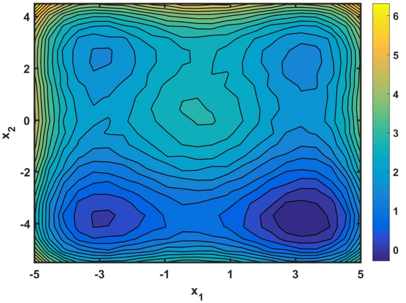
We consider the situation of a diffusive particle in ${\mathbb{R}}^{2}$ that is confined by the following periodically perturbed quadruple-well potential¹¹ 1 Eric Barth, private communication. shown in Figure 1

(6.6)		$\displaystyle V=$	$\displaystyle 0.01\left((x_{1}-0.1)^{4}-20x_{1}^{2}+(x_{2}+0.4)^{4}-20x_{2}^{2}\right.$
(6.6)			$\displaystyle+\left.10\sin(5x_{1})\cos(5x_{2})+x_{1}x_{2}+290.4\right)$

The potential has a deep energy well in the south-east of the $x_{1}$ - $x_{2}$ -plane, one slightly shallower well in the south-west and two even shallower wells in the north-west and north-east. The system is metastable, in that the time scale to reach the deepest potential energy well from any of the other three wells is of the order of the Arrhenius timescale $e^{\beta\Delta V_{\rm min}}\gg 1$ where $\Delta V_{\rm min}$ denotes the minimum energy barrier that a particle going from one well to the south-east well would have to overcome [14]. The various local minima of the potential energy surface that originate from the periodic perturbation do not have any significant effect on the transition rates between the main wells. The corresponding stationary density $\mu$ is shown in the upper left panel of Fig. 2. For moderate temperature ( $\beta=4.0$ ) essentially only the two main wells are populated, with considerably more weight on the deepest minimum (SE).

6.2. Finite difference discretization

Sine all coefficients in the FPE (6.2) are sufficiently smooth, we can discretize it using finite differences. Let $\Omega=(a,b)\times(c,d)$ , and consider the solution domain $D=\bar{\Omega}\times[0,T]\subset{\mathbb{R}}^{2}\times{\mathbb{R}}_{+}$ . On a bounded domain, probability conservation (6.3) requires that the outwards probability flux

J_{u}(\rho)=\beta^{-1}\nabla\rho+\rho(\nabla V-u)

across the boundary of the spatial domain is zero at any time. Letting $\nu$ denote the outward pointing normal to $\partial\Omega$ , the FPE (6.2) on $D$ reads

(6.7)	$\displaystyle\frac{\partial\rho}{\partial t}=\nabla\cdot\left(\beta^{-1}\nabla\rho+\rho(\nabla V-u)\right)\,,$	$\displaystyle(x,t)\in\Omega\times(0,T]$
	$\displaystyle 0=\nu\cdot J_{u}(\rho)\,,$	$\displaystyle(x,t)\in\partial\Omega\times[0,T]$
	$\displaystyle\rho_{0}=\rho\,,$	$\displaystyle(x,t)\in\Omega\times\{0\}\,.$

For simplicity we will discretize the equation on the uniform mesh

	$\displaystyle\Omega_{h}$	$\displaystyle:=\{(a+ih_{1},c+jh_{2})\;\colon 1<i<n_{1}-1,1<j<n_{2}-1\},$
	$\displaystyle\partial\Omega_{h}$	$\displaystyle:=\{(a+ih_{1},c+jh_{2})\;\colon 0\leq i\leq n_{1},0\leq j\leq n_{2}\}\setminus\Omega_{h},$

where $h_{1}=(b-a)/(n_{1}+1)$ and $h_{2}=(d-c)/(n_{2}+1)$ are the mesh sizes in $x_{1}$ and $x_{2}$ direction. Letting $w_{i,j}=\rho(x_{1,i},x_{2,j})$ with $(x_{1,i},x_{2,j})\in\Omega$ , we approximate the first and second derivatives in the usual way by centered finite differences, e.g.

(6.8)		$\displaystyle\left.\frac{\partial\rho}{\partial x_{1}}\right\|_{x=(x_{1,i},x_{2,j})}$	$\displaystyle\approx\frac{w_{i+1,j}-w_{i-1,j}}{2h_{1}}$
(6.8)		$\displaystyle\left.\frac{\partial^{2}\rho}{\partial x_{1}^{2}}\right\|_{x=(x_{1,i},x_{2,j})}$	$\displaystyle\approx\frac{w_{i+1,j}-2w_{i,j}+w_{i-1,j}}{h_{1}^{2}}\,.$

For sufficiently small mesh size $h=(h_{1},h_{2})$ , the finite difference discretization is known to preserve positivity, norm and stochastic stability. As a consequence, the stationary distribution of the discretized equation is the unique asymptotically stable fixed point and approximately equal to the stationary solution $\mu$ of the original equation, evaluated at the grid points; cf. [35].

In matrix-vector notation, the discretization of (6.7) can be compactly written as

(6.9)

\dot{v}=Av+\sum_{k=1}^{2}u_{k}N_{k}v\,,\quad v(0)=v_{0}\,

where $v\in{\mathbb{R}}^{n}$ with $n=n_{1}n_{2}$ is the column-wise tensorization of $(w_{i,j})_{i,j}$ , i.e. $v_{i+(j-1)n_{1}}=w_{i,j}$ , $A\in{\mathbb{R}}^{n\times n}$ is the discretization of the Fokker–Planck operator

\nabla\cdot\left(\beta^{-1}\nabla\rho+\rho\nabla V\right)=\beta^{-1}\Delta\rho+\nabla V\cdot\nabla\rho+(\Delta V)\rho

of the uncontrolled dynamics, and the $N_{i}$ are the discretization of the partial derivatives $\partial/\partial x_{i}$ on the tensorized grid, $u_{1}$ and $u_{2}$ are the components of $u$ .

By construction, $-A$ is an $M$ -matrix with a simple eigenvalue $0$ that corresponds to the discretized unique stationary distribution $\pi\approx\mu|_{\Omega_{h}}$ , all other eigenvalues have strictly negative real parts. This is in contrast to the spectral properties of the original operator that is symmetric (essentially self-adjoint) when considered on the appropriately weighted Hilbert space, i.e., all its eigenvalues are real. We observe, however, that the dominant eigenvalues are real when the discretization is sufficiently fine.

Tab. 1 gives the 12 smallest eigenvalues (by their magnitude) of the matrix $A$ and for a discretization of the domain $\Omega=(-6.0,6.0)\times(-5.5,6.5)$ with uniform mesh size $h_{1}=h_{2}=0.25$ ; the size of the resulting matrix $A$ is $2401\times 2401$ . The $L^{1}$ -deviation between the eigenvector $\pi$ to the eigenvalue $\lambda_{0}=0$ and $\mu$ evaluated at the grid points is smaller than $0.007$ . As the theory predicts, the matrix has 4 dominant eigenvalues close to $0$ (including $\lambda_{0}=0$ ) that are separated from the rest of the spectrum. Figure 2 shows the 4 dominant eigenvectors of $A$ , the first one being the stationary distribution that is essentially supported by the two deepest minima, the second one describing the dominant transition process between the deepest and the second deepest minimum, the third one representing the transitions between the second and the third deepest minimum and so on. The absolute values of the corresponding eigenvalues $\lambda_{1},\,\lambda_{2},\,\lambda_{3}<0$ represent (up to an error of order $\sqrt{\epsilon}$ ) the transition rates between the dominant potential energy wells. The fact that the subdominant eigenvalues appear in clusters of 4 has to do with the approximate four-fold symmetry of the potential. By tilting the potential towards one or several of the minima (thus flattening some of the other minima) the number of eigenvalues in the dominant cluster changes according to the number of resulting wells.

6.3. Stable input-output system in standard form

We first augment (6.9) by an output equation. To this end we introduce the observable $y=(y_{1},\ldots,y_{4})\geq 0$ denoting the probability for each of the four energy wells. The $y_{i}$ are given by summation of the density $v$ over all mesh points corresponding to the four quadrants of the $x_{1}$ - $x_{2}$ -plane, which, using the tensorized form of the equation, can be written as

(6.10)

y=Cx

for a matrix $C\in{\mathbb{R}}^{4\times n}$ . The discretized FPE is bilinear, but it is homogeneous, i.e., it does not contain a purely linear term “ $Bu$ ”, which implies that no state is reachable from the origin $v(0)=0$ .²² 2 Note that $v(0)=0$ is not a probability density, hence not an admissible starting point from a probabilistic point of view. To transform (6.9) into the standard form (2.1), we follow the procedure described in Sec. 5.2.

6.4. Numerical results

Here and throughout the following we will use the following short-hand notation when comparing results for the three approaches to model order reduction: BT stands for balanced truncation, as given by equation (4.5) in Sec. 4.3 whereas SP symbolizes the averaging principle derived from singular perturbation theory, as given by equations (4.9)–(4.10) in Sec. 4.4. Finally, H2 is the $\mathcal{H}_{2}$ -optimal model order reduction of Sec. 3.

The details of the following comparisons depend sensitively on the value of the parameter $\eta$ used for scaling of the control field $u(t)$ and matrices $N_{k}$ and $B$ , which is necessary to guarantee existence and uniqueness of controllability and observability Gramians, see Sec. 5.4. For the particular example of the FPE dynamics for inverse temperature $\beta=4$ investigated here, we use a value of $\eta=10$ consistently for all three approaches to model order reduction. Moreover, to stabilize the $A$ matrix we use here the projection method from Sec. 5.2. However, our results are practically unchanged when using the discounting approach described in Sec. 5.3 instead, assuming that the regularization parameter $\alpha$ is within a reasonable range.

The behavior of the $\mathcal{H}_{2}$ -error defined in (5.5) for the discretized FPE is shown in Fig. 3. Similarly for all of the three methods, this error displays a plateau value of approximately $10^{-5}$ for a reduced dimensionality of about $d\gtrsim 60$ . Upon further reduction of the dimensionality we observe a rapid increase over several orders of magnitude indicating a decreased quality when reducing overly. In most cases it is found that the $\mathcal{H}_{2}$ -error for the H2 method is slightly lower than for BT, which in turn is slightly lower than for the SP method.

While the $\mathcal{H}_{2}$ -error characterizes the error of model order reduction for the limiting case of an infinitely short pulse (Dirac-like) control field, it may be also of interest to compare full versus reduced order models for more realistically shaped control fields. As an example we consider here the Fokker–Planck dynamics, again for $\beta=4$ , induced by a Gaussian-shaped control pulse along the $x_{2}$ -direction

(6.11)

u_{2}(t)=a\exp\left(-\frac{(t-t_{0})^{2}}{2\sigma^{2}}\right)

centered at $t_{0}=150$ . Here $\sigma=\tau/\sqrt{8\log 2}$ is chosen to yield a full width at half maximum of $\tau=100$ which is on the same order of magnitude as the relaxation time to equally account for the aspects of controllability and observability. The time evolution of the four above-mentioned observables (populations of the quadrants of the $x_{1}$ - $x_{2}$ plane) is shown in Fig. 4. The amplitude $a=0.5$ of the pulse has been determined to drive approximately one half of the density from the lower minima (south) to the higher minima (north) at $t\approx 200$ . At later times, the populations return exponentially to their original values defined by the canonical density of Eq. (6.5).

Our numerical experiments show that the population dynamics for $d=100$ is still practically indistinguishable from calculations in full dimensionality. When further reducing the model order down to $d=50$ and $d=30$ , we observe that the quality of the SP method is superior to the BT or H2 method. However, despite of some minor differences, the overall performance of all three model order reduction schemes is impressive when considering that the original dimension of the problem is $n=2401$ . We observe that the $\mathcal{H}_{2}$ error occasionally drops below machine precision. These occurrences appear at random and are not reproducible (depending e.g. on the computer used for the numerical calculation) and therefore we attribute them to numerical artifacts and exclude the values in the corresponding plots.

We emphasize that replacing the reduced-order model by a coarse finite-difference discretization of the advection-dominated Fokker-Planck equation is not advisable. For example, using a mesh size $h_{1}=h_{2}=1.25$ , and thus 11 grid points per dimension, corresponding to a system of dimension $d=121$ , we find that the error in the stationary distribution (i.e. the eigenvector to the eigenvalue $\lambda_{0}=0$ ) is of order 1 and that none of the dominant eigenvalues is approximated. For even larger mesh size, the eigenvalues of the matrix $A$ cross the imaginary axis, resulting in an unstable system. Hence the recommended reduction strategy consists in first generating a sufficiently fine discretization of the original system and then reducing the dimension.

7. Liouville–von Neumann equation

As a second example we choose the dynamics of open $q$ –state quantum systems. Usually those are formulated in terms of a matrix representation of the reduced density operator, $\rho\in{\mathbb{C}}^{q\times q}$ , the diagonal and off-diagonal entries of which stand for populations and coherences, respectively. The time–evolution of $\rho$ is governed by a quantum master equation which, due to a formal similarity with the Liouville equation in classical mechanics, is termed Liouville–von Neumann (LvNE) equation [57, 19]

(7.1)

i\frac{\partial}{\partial t}\rho(t)={\mathcal{L}}_{H}\rho(t)+{\mathcal{L}}_{D}\rho(t)\,,

where we have used atomic units ( $\hbar=1$ ). The first Liouvillian on the right hand side represents the closed system quantum dynamics

(7.2)

{\mathcal{L}}_{H}\rho(t)=-i\left[H_{0}-\sum_{k}F_{k}(t)\mu_{k},\rho(t)\right]_{-}

where $[\cdot,\cdot]_{-}$ stands for a commutator and where the field–free system is expressed in terms of its Hamiltonian matrix $H_{0}$ . The system can be controlled through the interaction of its dipole moment matrices $\mu_{k}$ with electric field components $F_{k}(t)$ which is the lowest–order semiclassical expression for the interaction of a quantum system with an electromagnetic field. The second Liouvillian on the right hand side of (7.1) represents the interaction of the system with its environment thus accounting for time-irreversibility, i.e., dissipation and/or dephasing. A commonly used model for these processes is the Lindblad form [40]

(7.3)

{\mathcal{L}}_{D}\rho=i\sum_{c}\left(C_{c}\rho C_{c}^{\dagger}-\frac{1}{2}\left[C_{c}^{\dagger}C_{c},\rho\right]_{+}\right)\,,

where the index $c$ runs over all dissipation channels [18] and where $[\cdot,\cdot]_{+}$ stands for an anti–commutator. The Lindblad operators $C_{c}$ describe the coupling to the environment in Born-Markov approximation (weak coupling, no memory), typically chosen to be projectors

(7.4)

C_{c}=C_{i\leftarrow j}=\sqrt{\Gamma_{i\leftarrow j}}\,|i\rangle\langle j|

with rate constants (inverse times) $\Gamma_{i\leftarrow j}$ .

In order to cast the evolution equation (7.1) into the standard form of bilinear input-output systems (5.2) for deviations from the stationary solution, the density matrix $\rho$ has to be mapped onto a vector $x$ with $n=q^{2}$ components. Choosing the vectorization such that populations go in front of coherences offers the advantage that $A$ is blockdiagonal with block sizes $q$ and $(n-q)$ where the latter block is diagonal. Moreover, the upper left submatrix of $N$ is a zero matrix of size $q\times q$ . We note that typically both $A$ and $N$ are sparse matrices whereas $B$ and $C$ are not. For more details of the vectorization procedure and the associated construction of matrices $A$ , $N$ , $B$ , and $C$ from the LvNE, see Appendix A of Ref. [49].

With the Lindblad model introduced above, the LvNE (7.1) is trace-preserving (i.e., the sum of populations remains constant) and completely positive (i.e., the individual populations remain positive) thus ensuring the probabilistic interpretation of densities in quantum mechanics. Despite of the different discretization schemes used, the model bears many similarities with the discretized Fokker–Planck equation considered in Sec. 6, including the simple zero eigenvalue of the matrix $A$ .

7.1. Double well model system

We apply our model reduction approaches to dissipative quantum dynamics described by a (one–dimensional) asymmetric double well potential as presented in our previous work [49, Figure 1]. Our parameters are chosen such that there are six (five) stationary quantum states which are essentially localized in the left (right) well. We also include the first ten eigenstates above the barrier separating the wells which are delocalized while even higher states are not considered for simplicity. In total, the $q=21$ considered states lead to a density matrix with dimension $n=441$ . Thus, model order reduction can be mandatory, e.g., during a refinement of fields in optimal control.

In the present model simulations, the dependence of rate constants $\Gamma_{i\leftarrow j}$ with $j>i$ describing the decay of populations (and associated decoherence) are obtained from the model of Ref. [3] which employs only one adjustable parameter which we choose as $\Gamma\equiv\Gamma_{0\leftarrow 2}$ ; the rates for upward transitions ( $i>j$ ) are calculated from those for downward ones using the principle of detailed balance

(7.5)

\Gamma_{j\leftarrow i}=\exp\left(-\frac{E_{j}-E_{i}}{\Theta}\right)\Gamma_{i\leftarrow j},\quad j>i

where $E$ are the eigenvalues of the unperturbed Hamiltonian $H_{0}$ . Hence, the temperature $\Theta$ is the second parameter needed to set up matrix $A$ (assuming Boltzmann constant $k_{B}=1)$ . The external control of the quantum system is modeled within the semi-classical approximation of Eq. (7.2): The electric field $F(t)$ interacts linearly with the dipole moment $\mu$ which is assumed to be proportionate to the system coordinate of the double well system which is used to set up matrices $N$ and $B$ describing the controllability. To observe the system dynamics, we monitor the sums of the populations of the quantum states localized in the left and right well, and of the delocalized states over the barrier. These three quantities are used to construct the matrix $C$ describing the observability [49].

7.2. Numerical results

As was already noted for the FPE example, the performance of the model order reduction schemes depends sensitively on the value of the parameter $\eta$ used for scaling of the control field $u(t)$ and matrices $N_{k}$ and $B$ , see Sec. 5.4. For all examples from LvNE dynamics discussed here, we use a value of $\eta=3$ . In addition, the $A$ matrices are stabilized using the projection method introduced in Sec. 5.2. Again, all results are practically unchanged when using the discounting approach described in Sec. 5.3 instead.

We begin our discussion by considering the spectrum of the $A$ -matrix as displayed in Fig. 5. With increasing dimension reduction, more and more of the eigenvalues with lowest (most negative) real parts are eliminated first. As has been detailed in Appendix A of Ref. [49], those correspond to quantum states which decay fastest. Hence, the eigenvalues of $A$ with lowest real part are associated with lowest observability. At the same time, the order reduction tends to eliminate states with large imaginary part first. Those correspond to coherences between quantum states with large energy gaps for which the Franck-Condon (FC) factors are typically very low. Hence, the eigenvalues of $A$ with largest imaginary part are associated with lowest controllability. A noteworthy exception are the results for $d=30$ (green dots in Fig. 5) with real parts near zero. There, the imaginary parts (energy differences) near even multiples of $\approx 0.1$ can be assigned to ladder climbing within each of the wells of the double well potential, while odd multiples correspond to transitions between the minima. Because the FC factors for the former ones are larger, they are more likely to be preserved in dimension reduction due to their higher controllability. This is seen most clearly in the left panel of Fig. 5, i.e., for the BT method. In summary, the model order reduction confines the spectrum of $A$ to the lower (most controllable) and to the right (most observable) part of the complex number plane. In general, the results of the three different approaches (BT, SP, and H2 method) are very similar to each other.

To quantify the error introduced by model order reduction of the LvNE system, we consider the behavior of the $\mathcal{H}_{2}$ -error as defined in (5.5). Our results for various values of the relaxation rate $\Gamma$ (but constant temperature, $\Theta=0.1$ ) are shown in the left half of Fig. 6. The higher the value of the relaxation rate $\Gamma$ , the smaller is the ${\mathcal{H}}_{2}$ error and the earlier the error reaches a plateau at about $10^{-10}\ldots 10^{-9}$ . Hence, dimension reduction is more effective for open quantum systems with larger rate constants for relaxation (and associated decoherence). Furthermore, it is noted that the BT and the H2 method yield similar ${\mathcal{H}}_{2}$ errors at comparable computational effort so that there is no clear preference for either one of them.

Our results for various values of the temperature $\Theta$ (but constant relaxation, $\Gamma$ =0.1) are shown in the right half of Fig. 6. For low ( $\Theta=0.07$ ) and for medium ( $\Theta=0.1$ ) temperatures, the ${\mathcal{H}}_{2}$ error decreases with increasing dimensionality $r$ and again reaches a plateau. However, at higher temperature ( $\Theta=0.2$ ) the error decreases rapidly and reaches machine precision at $r\approx 100$ .

Again, in most cases the results for the different methods are close to each other, with the only exception being the lower temperature ( $\Theta=0.07$ ), where the $\mathcal{H}_{2}$ -error for the BT method is often found below that for the H2 method. At low temperature the system becomes less controllable, and this suggests that H2 does not always correctly capture the controllable states—which BT does by construction. As before in the Fokker–Planck example, we observe that the $\mathcal{H}_{2}$ error occasionally drops below machine precision. As these occurrences appear at random and are not reproducible (depending e.g. on the computer used for the numerical calculation), we attribute them to numerical artifacts and exclude the values in the corresponding plots.

Finally, an example for the time evolution of the three above-mentioned observables (populations) in the asymmetric double well system (relaxation rate $\Gamma=0.1$ and temperature $\Theta=0.1$ ) is investigated for the control field given in Eq. (6.11), here with $a=3$ , $t_{0}=15$ , and $\tau=10$ . The pulse drives the population, which is initially mainly in the left well of the potential, to delocalized quantum states over the barrier from where transitions to the right well are induced. The subsequent relaxation to the thermal distribution proceeds on a much longer time scale not shown here. In Fig. 7 we compare the results for full dimensionality ( $n=441$ ) with reduced dimensionality $d$ . While the results for $d=100$ are still essentially exact, the results for $d=50$ start to deviate notably. For $d=30$ only the BT method (left panel of Fig 7) reproduces the full dimensional ones qualitatively while SP method (center panel) as well as H2 method (right panel) fail completely.

8. Conclusions

In this paper, model reduction methods for bilinear control systems are compared, with a special focus on Fokker–Planck and Liouville–von Neumann equation. The methods can be categorized into balancing based (balanced truncation, singular perturbation) and interpolation based ( $\mathcal{H}_{2}$ optimization) reduction methods. While these methods have already been discussed in [2, 49, 9, 8, 24], our focus is on a direct and thorough comparison between all of them. Particularly, we draw the following conclusions with regard to computational complexity, accuracy and applicability to realistic bilinear dynamics.

8.1. Computational complexity

The computational effort of BT and SP is essentially determined by the solution of the two generalized Lyapunov equations (2.6) and (2.7). From a theoretical point of view, the complexity for solving these equations explicitly is $\mathcal{O}(n^{6}).$ On the other hand, an iterative approximation ([22]) as described in Sec. 5.5 with $r$ iteration steps only requires $\mathcal{O}(rn^{3})$ operations (due to solving the standard Lyapunov equations in each step by a direct solver such as the Bartels-Stewart algorithm by lyap in MATLAB). As an alternative, the generalized equations can be rewritten as a linear problem which can be solved, e. g., by the bi–conjugate gradient method where it is advantageous to use the solutions of the corresponding ordinary equations for pre-conditioning.

The effort of H2 is mainly due to the solution of two generalized Sylvester equations in each step of the bilinear iterative rational Krylov algorithm (BIRKA). In contrast to BT/SP, a direct solution of these equations requires “only” $\mathcal{O}(l^{3}n^{3})$ operations ( $l$ denoting the dimension of the reduced model). Similarly, the cost for an iterative procedure is less since the standard Sylvester equations can be handled efficiently for sparse system matrices. Hence, a single step of BIRKA is computationally less expensive than performing the balancing step in BT/SP. However, the overall cost for BIRKA obviously depends on the number of iteration steps that is needed until the fixed point iteration is (numerically) converged, see Sec. 3. Based on the numerical examples studied here, we can not report significant differences between all three methods.

8.2. Accuracy of reduced models

The overall performance of all three methods is very satisfactory. Both transient responses as well as spectral properties of the original model are faithfully reproduced by all reduced models (see Figs. 3–4 and 6–7. Despite the nature of H2, a significant difference of the quality (w.r.t. the $\mathcal{H}_{2}$ -norm) of the reduced models cannot be observed. Also, the (moderate) additional effort for SP instead of BT does not seem to lead to more accurate reduced models.

8.3. Unstable bilinear dynamics and scaling

Both BT/SP and H2 require the dynamics of the unperturbed system to be stable. The spectrum of the matrix $A$ representing the field-free FPE / LvNE dynamics is in the left half of the complex number plane, however, with an additional single eigenvalue zero. The effects of two different stabilization techniques, i.e. a shift of the spectrum of $A$ versus a splitting of stable and unstable parts leads to similarly accurate results (see Secs. 5.2 and 5.3). The latter approach however has the benefit that the bilinear dynamics are not changed by projecting onto the asymptotically stable part.

For the generalized Lyapunov and/or Sylvester equations to be solvable, the norms of the matrices $B$ and $N_{k}$ have to be kept below certain thresholds which is achieved by down-scaling these matrices and corresponding up-scaling of the control fields, cf. Sec. 5.4. This leaves the equations of motion invariant (but not the Gramians). Here we observe significantly different results depending on the choice/size of the scaling factor. In some cases, good results are obtained only for large scaling factors. However, we emphasize that large scaling factors drive the Gramians to those appearing for the linear(ized) system. For this reason, an automatic (large) choice of these factors is not recommended but has to be investigated for the problem under consideration on a case by case basis. From the numerical example, we believe that the scaling is a very important point for obtaining “optimal” reduced models.

8.4. Further issues

Another aspect related to the computation of the balancing transformation that we mention only for the sake of completeness is that it is often advisable to exploit sparsity and to use low-rank techniques that do not require to compute the full Gramians and their Cholesky factorization, one such example being the low-rank Cholesky factor ADI method [38, 13]. These methods require some fine tuning of the parameters to enforce convergence, but for example, in case of the Fokker–Planck equation for which the matrices $A$ and $N$ that are extremely sparse and the rank of the matrix $-BB^{T}$ is much smaller than the size of the matrices $A,N$ , there can be a considerable gain from using low-rank techniques.

Appendix A Stability of balanced and reduced systems

We now prove that the balancing transformation (4.1)–(4.2) preserves the stability of the submatrices $\tilde{A}_{11}$ and $\tilde{A}_{22}$ . The idea of the proof essentially follows [5, Thm. 7.9]; see also [11]. We confine our attention to $\tilde{A}_{22}$ , the stability of which is needed for the averaging principle to apply, and we stress that the proof readily carries over to the proof that $\tilde{A}_{11}$ is stable (Hurwitz). Let

(A.1)		$\displaystyle\tilde{A}$	$\displaystyle=\left(\begin{array}[]{cc}\tilde{A}_{11}&\tilde{A}_{12}\\ \tilde{A}_{21}&\tilde{A}_{22}\end{array}\right),\quad\tilde{N}_{k}=\left(\begin{array}[]{cc}\tilde{N}_{k,11}&\tilde{N}_{k,12}\\ \tilde{N}_{k,21}&\tilde{N}_{k,22}\end{array}\right),$
(A.1)		$\displaystyle\tilde{B}$	$\displaystyle=\left(\begin{array}[]{c}\tilde{B}_{1}\\ \tilde{B}_{2}\end{array}\right),\quad\tilde{C}=\left(\begin{array}[]{ll}\tilde{C}_{1}&\tilde{C}_{2}\end{array}\right)\,$

denote the coefficients of the balanced bilinear system for $\epsilon=1$ .

Lemma A.1.

Suppose that Assumptions 1–5 from pages 2.2 and 4 hold, and let the matrix of Hankel singular values $\Sigma$ be defined as in (4.1). If the submatrices $\Sigma_{1}$ and $\Sigma_{2}$ have disjoint spectra, $\lambda(\Sigma_{1})\cap\lambda(\Sigma_{2})=\emptyset$ , then

\lambda(\tilde{A}_{22})\subset{\mathbb{C}}_{-}\,,

where ${\mathbb{C}}_{-}$ denotes the open left complex half-plane.

Proof.

We first prove that the spectrum of $\tilde{A}_{22}$ lies in the closed left complex half-plane (including the imaginary axis). To this end note that (2.7) implies that

\tilde{A}_{22}\Sigma_{2}+\Sigma_{2}\tilde{A}_{22}^{*}+\sum_{k=1}^{m}\left(\tilde{N}_{k,22}\Sigma_{2}\tilde{N}^{*}_{k,22}+\tilde{N}_{k,21}\Sigma_{1}\tilde{N}^{*}_{k,12}\right)+\tilde{B}_{2}\tilde{B}_{2}^{*}=0\,.

Now let $v\in{\mathbb{C}}^{n-d}$ be an eigenvector of $\tilde{A}^{*}_{22}$ to the eigenvalue $\lambda\in{\mathbb{C}}$ , i.e. $\tilde{A}^{*}_{22}v=\lambda v$ . Multiplication of the last equation with $v^{*}$ and $v$ from the both sides yields

2\Re(\lambda)\big|\Sigma^{1/2}_{2}v\big|^{2}+\sum_{k=1}^{m}\left(\big|\Sigma_{2}^{1/2}\tilde{N}^{*}_{k,22}v\big|^{2}+\big|\Sigma_{1}^{1/2}\tilde{N}^{*}_{k,12}v\big|^{2}\right)+\big|\tilde{B}_{2}^{*}v\big|^{2}=0\,.

Noting that both $\Sigma_{1}$ and $\Sigma_{2}$ are positive definite, it follows that $\Re(\lambda)\leq 0$ , thus the eigenvalues of $\tilde{A}_{22}$ are in the left complex half-plane or on the imaginary axis.

As a second step we will demonstrate that indeed $\Re(\lambda)<0$ . We proceed by contradiction and suppose the contrary. Following [5], there exists a linear change of variables $x\mapsto Vx$ , $x\in{\mathbb{C}}^{n}$ , such that

V=\left(\begin{array}[]{cc}{\mathbf{1}}&{\mathbf{0}}\\ {\mathbf{0}}&V_{22}\end{array}\right)\,,\quad V_{22}\tilde{A}_{22}V_{22}^{-1}=\left(\begin{array}[]{cc}\hat{A}_{22}&{\mathbf{0}}\\ {\mathbf{0}}&\hat{A}_{33}\end{array}\right)\,,

with $\hat{A}_{22}$ having eigenvalues in ${\mathbb{C}}_{-}$ while the eigenvalues of $\hat{A}_{33}$ are pure imaginary. Under the change of variables, the balanced coefficients transform as follows:

	$\displaystyle\hat{A}$	$\displaystyle=\left(\begin{array}[]{ccc}\hat{A}_{11}&\hat{A}_{12}&\hat{A}_{13}\\ \hat{A}_{21}&\hat{A}_{22}&{\mathbf{0}}\\ \hat{A}_{31}&{\mathbf{0}}&\hat{A}_{33}\end{array}\right),\quad\hat{N}_{k}=\left(\begin{array}[]{ccc}\hat{N}_{k,11}&\hat{N}_{k,12}&\hat{N}_{k,13}\\ \hat{N}_{k,21}&\hat{N}_{k,22}&\hat{N}_{k,23}\\ \hat{N}_{k,31}&\hat{N}_{k,32}&\hat{N}_{k,33}\end{array}\right),$
		$\displaystyle\hat{B}=\left(\begin{array}[]{c}\hat{B}_{1}\\ \hat{B}_{2}\\ \hat{B}_{3}\end{array}\right),\quad\hat{C}=\left(\begin{array}[]{lll}\hat{C}_{1}&\hat{C}_{2}&\hat{C}_{3}\end{array}\right).$

Here $\hat{A}_{11}=\tilde{A}_{11}$ , $\hat{N}_{k,11}=\tilde{N}_{k,11}$ , $\hat{B}_{1}=\tilde{B}_{1}$ , and $\hat{C}_{1}=\tilde{C}_{1}$ . Accordingly, we have

\displaystyle\hat{Q}

\displaystyle=\left(\begin{array}[]{ccc}\Sigma_{1}&{\mathbf{0}}&{\mathbf{0}}\\ {\mathbf{0}}&\hat{Q}_{22}&\hat{Q}_{23}\\ {\mathbf{0}}&\hat{Q}_{32}&\hat{Q}_{33}\end{array}\right),\quad\hat{P}=\left(\begin{array}[]{ccc}\Sigma_{1}&{\mathbf{0}}&{\mathbf{0}}\\ {\mathbf{0}}&\hat{P}_{22}&\hat{P}_{23}\\ {\mathbf{0}}&\hat{P}_{32}&\hat{P}_{33}\end{array}\right).

Now consider the $(3,3)$ block of the generalized Lyapunov equation (2.7) for the controllability Gramian that reads

\hat{A}_{33}\hat{Q}_{33}+\hat{Q}_{33}\hat{A}_{33}^{*}+\sum_{k=1}^{m}(\hat{N}_{k,31}\;\hat{N}_{k,32}\;\hat{N}_{k,33})\hat{Q}(\hat{N}_{k,31}\;\hat{N}_{k,32}\;\hat{N}_{k,33})^{T}+\hat{B}_{3}\hat{B}_{3}^{*}=0

Now let $w$ be an eigenvector of $\hat{A}_{33}$ to a pure imaginary eigenvalue $\lambda=i\sigma$ . Then sandwiching the last equation with $w^{*}$ and $w$ from the left and from the right and iterating the argument from above, it follows that

\sum_{k=1}^{m}\big|\hat{Q}^{1/2}(\hat{N}_{k,31}\;\hat{N}_{k,32}\;\hat{N}_{k,33})^{T}w\big|^{2}+\big|\hat{B}_{3}^{*}w\big|^{2}=0\,,

which, by complete controllability and thus positivity of the matrix $\hat{Q}$ implies that $(\hat{N}_{k,31}\;\hat{N}_{k,32}\;\hat{N}_{k,33})^{T}w=0$ for all $k=1,\ldots,m$ . Therefore $\hat{B}_{3}^{*}w=0$ , and as we can pick $w$ to be any of the linearly independent eigenvectors of $\hat{A}_{33}$ we conclude that

\hat{B}_{3}={\mathbf{0}}\,,\quad\hat{N}_{k,31}={\mathbf{0}}\,,\quad\hat{N}_{k,32}={\mathbf{0}}\,,\quad\hat{N}_{k,33}={\mathbf{0}}\,,\quad k=1,\ldots,m\,.

By the same argument, using the adjoint Lyapunov equation (2.6) for the positive definite observability Gramian, it follows that

\hat{C}_{3}={\mathbf{0}}\,,\quad\hat{N}_{k,13}={\mathbf{0}}\,,\quad\hat{N}_{k,23}={\mathbf{0}}\,,\quad k=1,\ldots,m\,.

This entails that the $(2,3)$ block of the Lyapunov equation for $\hat{Q}$ has the form

\hat{A}_{22}\hat{Q}_{23}=\hat{Q}_{23}\hat{A}_{22}^{*}=0\,.

Hence $\hat{Q}_{23}={\mathbf{0}}$ and the analogous argument for the observability Gramian yields that $\hat{P}_{23}={\mathbf{0}}$ . Note that the Gramians are hermitian, i.e., $\hat{Q}_{23}=\hat{Q}_{32}^{*}$ and $\hat{P}_{23}=\hat{P}_{32}^{*}$ , which implies that the Gramians are block diagonal:

\displaystyle\hat{Q}

\displaystyle=\left(\begin{array}[]{ccc}\Sigma_{1}&{\mathbf{0}}&{\mathbf{0}}\\ {\mathbf{0}}&\hat{Q}_{22}&{\mathbf{0}}\\ {\mathbf{0}}&{\mathbf{0}}&\hat{Q}_{33}\end{array}\right),\quad\hat{P}=\left(\begin{array}[]{ccc}\Sigma_{1}&{\mathbf{0}}&{\mathbf{0}}\\ {\mathbf{0}}&\hat{P}_{22}&{\mathbf{0}}\\ {\mathbf{0}}&{\mathbf{0}}&\hat{P}_{33}\end{array}\right).

The Lyapunov equations for the $(1,3)$ blocks thus reads

\hat{A}_{13}\hat{Q}_{33}+\Sigma_{1}\hat{A}_{31}^{*}=0\,,\quad\hat{A}_{31}^{*}\hat{P}_{33}+\Sigma_{1}\hat{A}_{13}=0

Now multiplying the first of the two equations by $\Sigma_{1}$ from the left and substituting $\Sigma_{1}\hat{A}_{13}$ by $-\hat{A}_{31}^{*}\hat{P}_{33}$ yields $\hat{A}_{31}\hat{P}_{33}\hat{Q}_{33}=\Sigma_{1}^{2}\hat{A}_{31}^{*}$ . Interchanging the two Lyapunov equations we can show that $\Sigma_{1}^{2}\hat{A}_{13}^{*}=\hat{A}_{13}\hat{Q}_{33}\hat{P}_{33}$ . Now recall that the diagonal matrix $\Sigma^{2}$ contains the eigenvalues of $\hat{P}\hat{Q}$ or $\hat{Q}\hat{P}$ , and since the Gramians are block diagonal, it follows that $\Sigma_{2}^{2}$ contains the eigenvalues of $\hat{P}_{33}\hat{Q}_{33}$ or $\hat{Q}_{33}\hat{P}_{33}$ . By the assumption that $\Sigma_{1}$ and $\Sigma_{2}$ have no eigenvalues in common, we conclude that

\hat{A}_{13}={\mathbf{0}}\,,\quad\hat{A}_{31}={\mathbf{0}}\,.

This shows that the matrix $\hat{A}$ the form

\hat{A}=\left(\begin{array}[]{ccc}\hat{A}_{11}&\hat{A}_{12}&{\mathbf{0}}\\ \hat{A}_{21}&\hat{A}_{22}&{\mathbf{0}}\\ {\mathbf{0}}&{\mathbf{0}}&\hat{A}_{33}\end{array}\right),

which together with $\hat{B}_{3}={\mathbf{0}}$ and $\hat{C}_{3}={\mathbf{0}}$ violates the assumption of complete controllability and observability on 4. Hence $\tilde{A}_{22}$ cannot have eigenvalues on the imaginary axis, in other words: $\lambda(\tilde{A}_{22})\subset{\mathbb{C}}_{-}$ . ∎

Consequences of Lemma A.1 are the analogous statements for the matrix $\tilde{A}_{11}$ and the Schur complement of $\tilde{A}_{22}$ .

Corollary A.2.

Under the assumptions of Lemma A.1 it holds that

\lambda(\tilde{A}_{11})\subset{\mathbb{C}}_{-}\,.

Proof.

The proof is a simple adaption of the one of Lemma A.1 and [11, Thm 2.2]. ∎

Corollary A.3.

Under the assumptions of Lemma A.1 it holds that

\lambda(\tilde{A}_{11}-\tilde{A}_{12}\tilde{A}_{22}^{-1}\tilde{A}_{21})\subset{\mathbb{C}}_{-}\,.

Proof.

The assertion follows from Corollary A.2 by noting that the reciprocal system

\big(\hat{A},\hat{N}_{k},\hat{B},\hat{C}\big):=\big(\tilde{A}^{-1},\tilde{A}^{-1}\tilde{N}_{k},\tilde{A}^{-1}\tilde{B},-\tilde{C}\tilde{A}^{-1}\big)

is balanced if and only if $(\tilde{A},\tilde{N}_{k},\tilde{B},\tilde{C})$ is balanced, with

\hat{A}_{11}=\tilde{A}_{11}-\tilde{A}_{12}\tilde{A}_{22}^{-1}\tilde{A}_{21}\,.

∎

Remark A.4.

Note that $\hat{N}_{k}=\tilde{N}_{k,11}-\tilde{N}_{k,12}\tilde{A}_{22}^{-1}\tilde{A}_{21}$ is not the (1,1) block of the matrix $\tilde{A}^{-1}\tilde{N}_{k}$ , but rather the (1,1) coefficient of the matrix $\tilde{N}_{k}\tilde{A}^{-1}$ unless $\tilde{A}$ and $\tilde{N}$ commute. This has been pointed out in [46], and as a consequence, the singular perturbation approximation (4.9)–(4.10) is not the truncation of the reciprocal system as is the case for linear systems. Yet this does not affect the above argument and hence the stability of the Schur complement $\hat{A}=\tilde{A}_{11}-\tilde{A}_{12}\tilde{A}_{22}^{-1}\tilde{A}_{21}$ .

References

[1] M. I. Ahmad, U. Baur, and P. Benner. Implicit Volterra series interpolation for model reduction of bilinear systems. J. Comput. Appl. Math., 316(C):15–28, 2017.
[2] S. Al-Baiyat and M. Bettayeb. A new model reduction scheme for k-power bilinear systems. Proc. 32nd IEEE Conf. Decis. Control, 32:22–27, 1993.
[3] I. Andrianov and P. Saalfrank. Theoretical study of vibration–phonon coupling of H adsorbed on a Si(100) surface. J. Chem. Phys., 124:034710, 2006.
[4] M. Annunziato and A. Borzi. A Fokker–Planck control framework for multidimensional stochastic processes. J. Comp. Appl. Math., 237(1):487 – 507, 2013.
[5] A. Antoulas. Approximation of Large-Scale Dynamical Systems. SIAM, Philadelphia, 2005.
[6] Z. Bai and D. Skoogh. A projection method for model reduction of bilinear dynamical systems. Linear Algebra Appl., 415:406–425, 2006.
[7] U. Baur, P. Benner, and L. Feng. Model order reduction for linear and nonlinear systems: A system-theoretic perspective. Arch. Computat. Methods Eng., 21(4):331–358, 2014.
[8] P. Benner and T. Breiten. Interpolation-based $\mathcal{H}_{2}$ -model reduction of bilinear control systems. SIAM J. Matrix Anal. Appl., 33:859–885, 2012.
[9] P. Benner and T. Damm. Lyapunov equations, energy functionals, and model order reduction. J. Control Optim., 49:686–711, 2011.
[10] P. Benner and T. Damm. Lyapunov equations, energy functionals, and model order reduction. J. Control Optim., 49:686–711, 2011.
[11] P. Benner, T. Damm, M. Redmann, and Y. Rodriguez Cruz. Positive operators and stable truncation. Linear Algebra Appl., 491:74–87, 2016.
[12] P. Benner, S. Gugercin, and K. Willcox. A survey of projection-based model reduction methods for parametric dynamical systems. SIAM Review, 57(4):483–531, 2015.
[13] P. Benner, P. Kürschner, and J. Saak. Efficient handling of complex shift parameters in the low-rank cholesky factor ADI method. Numerical Algorithms, 62(2):225–251, 2013.
[14] N. Berglund. Kramers’ law: Validity, derivations and generalisations. Markov Processes Relat. Fields, 19:459–490, 2013.
[15] C. Boess, A. Lawless, N. Nichols, and A. Bunse-Gerstner. State estimation using model order reduction for unstable systems. Computers & Fluids, 46:155–160, 2011.
[16] T. Breiten and T. Damm. Krylov subspace methods for model order reduction of bilinear control systems. Syst. Control. Lett., 59:443–450, 2010.
[17] T. Breiten, K. Kunisch, and L. Pfeiffer. Control strategies for the Fokker-Planck equation. Technical report, University of Graz, 2016.
[18] H.-P. Breuer, W. Huber, and F. Petruccione. Stochastic wave-function method versus density matrix: a numerical comparison. Comp. Phys. Comm., 104:46–58, 1997.
[19] H.-P. Breuer and F. Petruccione. The theory of open quantum systems. Oxford University Press, Oxford, 2002.
[20] M. Condon and R. Ivanov. Empirical balanced truncation for nonlinear systems. J. Nonlinear Sci., 14:405–414, 2004.
[21] M. Condon and R. Ivanov. Nonlinear systems – Algebraic Gramians and model reduction. Int. J. Comp. Math., 24:202–219, 2005.
[22] T. Damm. Direct methods and ADI-preconditioned Krylov subspace methods for generalized Lyapunov equations. Numerical Linear Algebra with Applications, 15:853–871, 2008.
[23] N. de Souza. Pulling on single molecules. Nature Meth., 9:873–877, 2012.
[24] G. Flagg. Interpolation Methods for the Model Reduction of Bilinear Systems. PhD Thesis, Virginia Tech, 2012.
[25] G. Flagg and S. Gugercin. Multipoint volterra series interpolation and $\mathcal{H}_{2}$ optimal model reduction of bilinear systems. SIAM Journal on Matrix Analysis and Applications, 36(2):549–579, 2015.
[26] V. Gaitsgory. Suboptimization of singularly perturbed control systems. SIAM J .Control Optim., 30(5):1228–1249, 1992.
[27] G. Grammel. Averaging of singularly perturbed systems. Nonlinear Analysis, 28:1851–1865, 1997.
[28] S. Gugercin, A. Antoulas, and S. Beattie. $\mathcal{H}_{2}$ model reduction for large-scale dynamical systems. SIAM Journal on Matrix Analysis and Applications, 30(2):609–638, 2008.
[29] C. Hartmann, B. Schäfer-Bung, and A. Zueva. Balanced averaging of bilinear systems with applications to stochastic control. J. Control Optim., 51:2356–2378, 2013.
[30] C. Hartmann and C. Schütte. Efficient rare event simulation by optimal nonequilibrium forcing. J. Stat. Mech. Theor. Exp., 2012(11):P11004, 2012.
[31] C. Hartmann, V. Vulcanov, and C. Schütte. Balanced truncation of linear second-order systems: A Hamiltonian approach. Multiscale Model. Simul., 8(4):1348–1367, 2010.
[32] G. Hummer and A. Szabo. Free energy profiles from single-molecule pulling experiments. Proc. Natl. Acad. Sci. USA, 107(50):21441–21446, 2010.
[33] A. Isidori. Direct construction of minimal bilinear realizations from nonlinear input-output maps. IEEE Trans. Autom. Control, 18:626–631, 1973.
[34] S. Lall, J. Marsden, and S. Glavaški. A subspace approach to balanced truncation for model reduction of nonlinear control systems. Int. J. Robust Nonlinear Control, 12:519–535, 2002.
[35] J. C. Latorre, P. Metzner, C. Hartmann, and C. Schütte. A structure-preserving numerical discretization of reversible diffusions. Commun. Math. Sci., 9(4):1051 – 1072, 2011.
[36] C. Le Bris, Y. Maday, and G. Turinici. Towards efficient numerical approaches for quantum control. In A. Bandrauk, M. Delfour, and C. Le Bris, editors, Quantum Control: mathematical and numerical challenges, volume 33 of CRM Proceedings & Lecture Notes, pages 127–142. American Mathematical Society, 2002.
[37] T. Lelièvre and G. Stoltz. Partial differential equations and stochastic methods in molecular dynamics. Acta Numerica, 25:681–880, 2016.
[38] J.-R. Li and J. White. Low-rank solution of Lyapunov equations. SIAM Review, 46(4):693–713, 2004.
[39] Y. Lin, L. Bao, and Y. Wei. Order reduction of bilinear MIMO dynamical systems using new block Krylov subspaces. Comput. Math. Appl., 58:1093–1102, 2009.
[40] G. Lindblad. On the generators of quantum dynamical semigroups. Comm. Math. Phys., 48:119 – 130, 1976.
[41] W. E. Moerner. Nobel lecture: Single-molecule spectroscopy, imaging, and photocontrol: Foundations for super-resolution microscopy. Rev. Mod. Phys., 87:1183–1212, 2015.
[42] B. Moore. Principal component analysis in linear system: controllability, observability and model reduction. IEEE Trans. Automat. Control, AC-26:17–32, 1981.
[43] R. O’Malley. Singular Perturbation Methods for Ordinary Differential Equations. Springer, New York, 1991.
[44] M. Petreczky, R. Wisniewski, and J. Leth. Moment matching for bilinear systems with nice selections. IFAC-PapersOnLine, 49(18):838 – 843, 2016.
[45] J. Phillips. Projection-based approaches for model reduction of weakly nonlinear, time-varying systems. IEEE T. Comput. Aided. D., 22:171–187, 2003.
[46] M. Redmann and P. Benner. Singular perturbation approximation for linear systems with Lévy noise. Max Planck Institute Magdeburg Preprints, MPIMD/15-22:1–15, 2015.
[47] L. Rey-Bellet. Open classical systems. In S. Attal, A. Joye, and C.-A. Pillet, editors, Open Quantum Systems II: The Markovian Approach, pages 41–78. Springer Berlin Heidelberg, 2006.
[48] W. Rugh. Nonlinear System Theory. The Johns Hopkins University Press, 1982.
[49] B. Schäfer-Bung, C. Hartmann, B. Schmidt, and C. Schütte. Dimension reduction by balanced truncation: Application to light-induced control of open quantum systems. J Chem. Phys., 135(1):014112, 2011.
[50] B. Schmidt and C. Hartmann. Wavepacket: A MATLAB package for numerical quantum dynamics. II: Open quantum systems and optimal control. Comp. Phys. Comm., in preparation, 2017.
[51] B. Schmidt and U. Lorenz. Wavepacket: A MATLAB package for numerical quantum dynamics. I: Closed quantum systems and discrete variable representations. Comp. Phys. Comm., 213:223–234, 2017.
[52] T. Siu and M. Schetzen. Convergence of Volterra series representation and BIBO stability of bilinear systems. Int. J. Syst. Sci., 22(12):2679–2684, 1991.
[53] A. K. Tiwari, K. B. Møller, and N. E. Henriksen. Selective bond breakage within the HOD molecule using optimized femtosecond ultraviolet laser pulses. Phys. Rev. A, 78:065402, 2008.
[54] A. Vigodner. Limits of singularly perturbed control problems with statistical dynamics of fast motions. SIAM J. Control Optim., 35(1):1–28, 1997.
[55] E. Wachspress. Iterative Solution of the Lyapunov matrix equation. Appl. Math. Lett., 1:87–90, 1988.
[56] F. Watbled. On singular perturbations for differential inclusions on the infinite interval. J. Math. Anal. Appl., 310(2):362 – 378, 2005.
[57] U. Weiß. Quantum dissipative systems, volume 10 of Series in Modern Condensed Matter Physics. World Scientific, Singapore, 1999.
[58] D. Wilson. Optimum solution of model-reduction problem. Proceedings of the Institution of Electrical Engineers, 117(6):1161–1165, 1970.
[59] A. Zewail. Femtochemistry: Chemical reaction dynamics and their control. In P. Gaspard and I. Burghardt, editors, Advances in Chemical Physics: Chemical Reactions and their Control on the Femtosecond Time Scale: 20th Solvay Conference on Chemistry, volume 101, pages 103–108. John Wiley & Sons, Hoboken, NJ, USA, 1997.
[60] L. Zhang and J. Lam. On $H_{2}$ model reduction of bilinear systems. Automatica, 38:205–216, 2002.
[61] W. Zhang, H. Wang, C. Hartmann, M. Weber, and C. Schütte. Applications of the cross-entropy method to importance sampling and optimal control of diffusions. SIAM J. Sci. Comput., 36(6):A2654–A2672, 2014.

	BT method				H2 method
full	$d=200$	$d=100$	$d=50$	$d=25$	$d=200$	$d=100$	$d=50$	$d=25$
-0.0000	-0.0000	-0.0000	-0.0000	-0.0000	-0.0000	-0.0000	-0.0000	-0.0000
-0.0037	-0.0037	-0.0037	-0.0037	-0.0037	-0.0037	-0.0037	-0.0037	-0.0037
-0.0073	-0.0073	-0.0073	-0.0073	-0.0074	-0.0073	-0.0073	-0.0073	-0.0074
-0.0118	-0.0118	-0.0118	-0.0118	-0.0118	-0.0118	-0.0118	-0.0118	-0.0118
-0.3266	-0.3266	-0.3265	-0.3260	-0.3264	-0.3266	-0.3265	-0.3255	-0.3263
-0.3303	-0.3303	-0.3297	-0.3294	-0.3504	-0.3303	-0.3298	-0.3298	-0.3629
-0.3358	-0.3358	-0.3353	-0.3423	-0.5455	-0.3358	-0.3349	-0.3432	-0.5450
-0.3447	-0.3447	-0.3447	-0.3432	-0.5582	-0.3447	-0.3445	-0.3432	-0.6058
-0.5421	-0.5421	-0.5422	-0.5434	-0.6083	-0.5421	-0.5412	-0.5435	-0.6336
-0.5453	-0.5452	-0.5455	-0.5606	-0.6487	-0.5452	-0.5450	-0.5622	-0.6676
-0.5666	-0.5665	-0.5657	-0.5867	-0.7683	-0.5665	-0.5663	-0.5888	-0.7791
-0.5948	-0.5948	-0.5951	-0.6107	-0.8003	-0.5948	-0.5951	-0.6192	-0.8052

Table 1. Lowest twelve eigenvalues (in magnitude) of the discretization matrix

A

of the FPE example for inverse temperature

\beta=4

showing three clusters of four members each. Comparison of full versus reduced dynamics using the BT and H2 method. Results for the SP method (not shown) are very close to those for the BT method. For all practical purposes, the reduced systems for

d=200

are virtually indistinguishable from the full-rank system.

Refer to caption — Figure 1. Periodically perturbed quadruple-well potential (6.6) used in our FPE example.

Figure 6.

{\mathcal{H}}_{2}

error versus reduced dimensionality

d

for the LvNE example. Simulation results for which the error has dropped below machine precision are considered numerical artifact and thus are not shown. Left: For various values of the relaxation rate

\Gamma

(for constant temperature,

\Theta=0.1

) . Right: For various values of the temperature

\Theta

(for constant relaxation,

\Gamma=0.1

)

Model reduction of controlled Fokker–Planck and Liouville–von Neumann equations

Abstract.

Key words and phrases:

1. Introduction

2. Bilinear control systems

2.1. Reduced-order models

2.2. Standing assumptions

3. ℋ2\mathcal{H}_{2} optimal model reduction of bilinear systems

Definition 3.1.

4. Balanced model reduction for bilinear systems

4.1. Singularly perturbed bilinear systems

4.2. An averaging principle for bilinear systems

4.3. Balanced truncation

4.4. Singular perturbation

Theorem 4.1.

Remark 4.2.

5. Numerical details

5.1. Structured bilinear systems

5.2. Sparsity preserving projection

5.3. Discounting the system state

5.4. Scaling the control fields

5.5. Calculation of the ℋ2\mathcal{H}_{2} error

5.6. Software

6. Fokker–Planck equation

6.1. Metastable model system

6.2. Finite difference discretization

6.3. Stable input-output system in standard form

6.4. Numerical results

7. Liouville–von Neumann equation

7.1. Double well model system

7.2. Numerical results

8. Conclusions

8.1. Computational complexity

8.2. Accuracy of reduced models

8.3. Unstable bilinear dynamics and scaling

8.4. Further issues

Appendix A Stability of balanced and reduced systems

Lemma A.1.

Proof.

Corollary A.2.

Proof.

Corollary A.3.

Proof.

Remark A.4.

References

3. $\mathcal{H}_{2}$ optimal model reduction of bilinear systems

5.5. Calculation of the $\mathcal{H}_{2}$ error