Window for Efimov physics for few-body systems with finite-range interactions
Abstract
We investigate the two lowest-lying weakly bound states of bosons as functions of the strength of two-body Gaussian interactions. We observe the limit for validity of Efimov physics. We calculate energies and second radial moments as functions of scattering length. For identical bosons we find that two -body states appear before the -body ground states become bound. This pattern ceases to exist for where the size of the ground state becomes smaller than the range of the two-body potential. All mean-square-radii for remain finite at the threshold of zero binding, where they vary as with for ground and excited states, respectively. Decreasing the mass of one particle we find stronger binding and smaller radii. The identical particles form a symmetric system, while the lighter particle is further away in the ground states. In the excited states we find the identical bosons either surrounded or surrounding the light particle for few or many bosons, respectively. We demonstrate that the first excited states for all strengths resemble two-body halos of one particle weakly bound to a dense -body system for . This structure ceases to exist for .
I Introduction
The original Efimov effect [1, 2] describes the three-body structures using a single two-body parameter, the scattering length. Three identical bosons form infinitely many bound states with an accumulation point at the two-body scattering threshold where the scattering length approach infinity. The Efimov effect has universality and scale invariance as important concepts, and from generalizing these concept emerges Efimov physics which we in this article understand as the quantum physics where universality and scale independence apply.
We define universality as independence upon the shape of the interparticle potential, hence any interparticle model-potential should yield the same results. Scale invariance means independence upon the length scale of the system, hence the Efimov physics should be applicable on nuclei, atomic or any other scale. These concepts are unfortunately often only implicitly defined and with the meaning exchanged. Closely related to the Efimov effect is Borromean binding. This refers to a bound three-body system where none of the subsystems is bound. Thus removing just one of the bodies in such a system would make it unbound. This is often pictured classically by the three Borromean rings. Borromean systems often have large spatial extension and are weakly bound. Thus their structure is determined solely by the binding energy, which makes them good candidates for universality.
Efimov originally suggested that the effect could be found in nuclei, however the evidence was first reported for an ultra cold gas of caesium atoms using their three-body recombination rates [3]. It has since been observed in other ultracold gases of alkali metals (potassium and lithium) by exploiting Feshbach resonances to vary the effective two-body interaction [4, 5, 6], and more recently also in the Helium trimer [7].
Following the realization of the Efimov effect, much effort has been put into Efimov physics in general [8, 9, 10], expanding it beyond three identical bosons. These concepts are presented in the following two subsections.
I.1 Efimov physics beyond three bosons
Three years after Efimov predicted the effect, it was proven that there is no true Efimov effect for [11]. It was later predicted that each Efimov state is accompanied by two universal Borromean tetramer () states [12, 13]. This has been confirmed experimentally [6, 14], which therefore raises the question, whether this pattern continues for higher . Theoretical calculations for have been made, which predict that the pattern of two state accompany each universal ground state at least for [15, 16, 17, 18, 19, 20, 21, 22, 23, 24]. Experimental evidence that two Borromean pentamer () states does accompany the ground tetramer state have been reported [25].
Many calculations exploit the simplicity of zero-range interactions with two well-known principle problems, that is, the necessary regularization due to the small distance divergence and the missing finite range of a realistic interaction. The latter short-coming is essential in investigations touching upon or searching for the limits of Efimov physics. Quantum states with a substantial part located inside the range of the potential between neighboring particles must depend on the characteristics of the potential and consequently they cannot be universal. It is therefore essential to employ a finite-range potential for such investigations. Once the range is introduced in the practical calculations, the radial shape is unimportant for investigations of Efimov physics when the range of the potential is much smaller than the scattering length of the system. We shall use a Gaussian shape throughout this paper.
In Section III of this paper we present results for ground and first excited states for systems of identical bosons. This is done via numerical calculations using correlated Gaussian expansion determined by stochastic variation which is briefly described in Section II.1. We vary binding energies from zero to well-bound to investigate the limits for validity of universality.
The structure of -body systems is usually examined by calculating the pair-distribution function [18, 19, 26], however in this paper we present the actual radius of the system, and the average distance between the nearest neighboring particles for the ground and first excited state. For universality to apply we would require these to remain larger than the range of the potential. As increases these distances become shorter and hence we would expect that universality is broken at some .
For illustrative purposes we compare in Section IV our numerical calculations with schematic models. We compare with analytic harmonic oscillator results and estimates from Gaussian approximations of the true density distributions.
I.2 Efimov physics beyond identical bosons
The Efimov effect does not only occur for three identical bosons, but also for other three-body systems, with large scattering lengths. Efimov himself considered particles of different mass, and showed that the effect occurs for any mass ratio between the three particles [27]. This has been verified experimentally using alkali atoms of different mass, rubidium and potassium in [28] and caesium and lithium in [29, 30]. The scaling between the universal states of the system only depends on the mass ratio of the particles, making this quantity the parameter of interest when investigating non-identical particle systems. Mass asymmetric systems have been studied rather extensively both experimentally, [28, 31, 29, 30, 32, 33, 34, 35, 36] and theoretically [37, 38, 39, 40, 41, 42]. Lately it has even been discovered that a so-called super-Efimov effect among fermions in two dimensions [43, 44, 45, 46, 47, 48, 49], and also Efimov scaling phenomena in the dynamics of a strongly-interacting many-body Fermi gas [50].
Theoretical calculations for more than three bosons of different mass provide energy scalings between different states [26, 51], while leaving the spatial configuration unpredicted. In Section V we thus investigate the three- to seven-body systems where the mass of one particle is varied, with focus on resolving the spatial configuration between the particles. We numerically calculate the ground and first excited states of these systems, where we vary the mass of one of the particles until its mass is a twentieth of the rest of the particles. We investigate the systems at the unitarity limit (infinite two-body scattering length) for scattering between unequal pairs of particles, while also maintaining a large scattering length for pairs of identical particles.
According to Efimov there should also be Efimov states for one heavy particle and two lighter particles. However, such Efimov states would be very loosely bound and are hence suppressed in low energy Efimov experiments [30]. Efimov systems with one heavy particle are not only experimentally difficult to produce, they are also difficult to calculate numerically again due to the weak binding. The same is true for more than three particles. Hence we focus on systems where one of the particles has less mass than all the other particles.
II Formulation of problem
For the first part of this paper we consider identical bosons, of mass , with coordinates and moment . We restrict the particles to interact only via two-body short-range potentials. Hence the Hamiltonian becomes
| (1) |
where and is the kinetic energy of the uninteresting decoupled center-of-mass motion.
In the second part of this paper where the mass of one of the particles, is varied, the Hamiltonian becomes
| (2) | ||||
where is the interaction between the identical (heavy-heavy) particles, and is the interaction between interspecies (heavy-light) particles. For the present calculations we will however assume that and therefor omit the subscript.
As we are interested in universality we can in principle choose any finite-range two-body potential. For simplicity we choose a Gaussian potential, such that the interaction between the th and th particle becomes
| (3) |
where is the potential strength, which is tuned in order to change the scattering length, , of the two-body system. The range of the potential, , is the characteristic length scale of the interaction, and together with the characteristic energy
| (4) |
where is the two-body reduced mass, it defines the universal regime, by requiring that the energies are much smaller and the length scales much larger than . Since we consider a finite-range potential, we expect some range-corrections [52, 53] compared to a zero-range potential. We also note that the finite-range potential implies that we do not need to provide a three-body cut-off at short-range of the order the van der Waals length [54, 55, 56, 57, 58, 59, 60, 61, 62, 63, 64, 65].
II.1 The stochastic variational method
All numerical calculations are done using the stochastically correlated Gaussians as trail functions
| (5) |
where the parameters are stochastically chosen. These trial functions are chosen since they are easily generalized to -body problems, and approximate all wave functions well. Furthermore they make an analytical calculation of matrix elements possible. Lastly the functions are spherically symmetric hence the calculated system has the total angular momentum equal zero.
A basis of these trial functions is initially chosen stochastically. The Generalized Ritz Theorem ensures that the expectation value of the Hamiltonian, restricted to the subspace of the the stochastically chosen trial functions, is always above the actual energy. Testing for a number of different sets of trial functions, the basis which yields the lowest energy is chosen, and the size of the basis is increased by one. Increasing the size of the basis will alway decrease the variational energy, and thus bring it closer to the exact value. Once again different sets of trial functions are tested and the one yielding the lowest energy is chosen, and such the process continues until the expectation value of the energies stabilizes and the calculation is stopped. At this point the basis of trial functions approximate the actual Hilbert space of the system, and thus other quantities of interest can be reliably calculated.
Since we are indeed approximating the Hilbert space we expect some numerical imprecision. These imprecisions are larger for more excited states and closer to the threshold of binding as these become more difficult to calculate. A method for lessening this numerical noise is to increase the basis of trial functions, however as the computational difficulty of this method increases as the square of the number of trial functions, this cannot continue forever. All numerical noise cannot be eliminated, and we allow some imprecision in the results appearing as small fluctuations. [66, 67]
III Identical particles

We consider -body systems of identical particles interacting pairwise with a Gaussian potential, Eq. 3. The particles may have integer or half-integer spin but we assume the interaction is spin independent. Thus the spatial wave function should be supplemented by the spin part and the total symmetry correspondingly derived.
We start numerically by using a basis of a few hundred trial functions. When we approach the threshold of binding a larger basis is needed since the systems are very weakly bound and often spatially extended. Shifting away from the threshold towards more binding, convergence is reached with a smaller basis. In order to further improve the convergence of the calculation the stochastically chosen parameter is steered towards numerically larger values near threshold, as the stochastically parameter is directly related to the spatial extend of the system.
III.1 Energies
We calculate the energies and two-body scattering lengths of the systems for different potential strengths, . We plot the -body energies as functions of the square of the inverse scattering length (a measure of the two-body energy) in Fig. 1 for . Following the by now established tradition, the axes in Fig. 1 has been scaled in order to increase visibility.
We first notice that both trimer states lie below the dimer ground state. We do not calculate more trimer states as only the two first states for all other are of interest in this paper, but infinitely many trimer states exist there below the dimer continuum as Efimov predicted. The binding of the excited state increases slower than the dimer binding energy, which is reached at some point after the dimer has become bound.
In order to assess the effect of the finite-range interaction we calculate the scaling factor defined here as the ratio between square roots of energies between the two lowest trimer states. Between the two lowest states we find this value numerically equal at unitarity i.e. where the dimer binding is zero. This should be compared to the value for a zero-range interaction found analytically to be
| (6) |
where . This is however the scaling factor of when approaches infinity. Since we are only dealing with the two lowest states, we should expect that the numerical scaling factor deviates some what from the analytical result in Eq. 6. The discrepancy in the scaling factors can be attributed to the finite range of the potential. This is due to the fact that even though the scattering length might be infinite, the size of the system is not. In column six and seven of Table 1 the average distances between the nearest neighboring particles are presented at the threshold of binding. For the two lowest trimer states these distances 5.9 and 50 times the range of the potential respectively. At the unitary limit these distances are even smaller, as seen on Fig. 2. Thus the finite range is responsible for the discrepancy between these scaling factors. We further compare our results with [68], who also calculates this scaling factor with a two-body finite Gaussian interaction, and finds , in good agreement with our result. The relation for the higher-lying excited trimer states would asymptotically approach the analytic result.
The behavior is completely different for . The attraction needed for binding decreases with increasing , and the spectra for each are limited to finite numbers below the trimer threshold. It is therefore inevitable that only a finite number of -body states can appear before the trimer becomes bound. The Efimov effect is not present for . Still a number of relations and properties exist. The excited states for each can appear with mixed spatial symmetry but the ground states are always symmetric. The first excited state is often also symmetric and these two states are therefore the solutions for identical bosons. We shall confine ourselves to this symmetry and these two lowest-lying states.
The two lowest states of the tetramer () boson system both lie below the ground state of the trimer system as seen in Fig. 1. This is in agreement with other numerical [69, 12, 13, 70] and experimental [14] investigations. The spacing strongly indicates that the second excited state, most likely of mixed spatial symmetry, would appear above the trimer threshold.
Furthermore our results indicate that this behavior continues for . Two pentamer () states accompany the ground state of the tetramer system, and the first excited state of the pentamer system lies so close to the ground state of the tetramer state, that it again seems improbable to find a second excited pentamer state below the tetramer threshold.
We now add one more particle to study the hexamer () system. The behavior is precisely repeated and we find two states below the pentamer ground state. This pattern is also found in a previous work [21], where a three-body interaction also is shown to move the first excited states for both above the -thresholds for binding. We maintain the use of only two-body interactions throughout this paper. Here it should be mentioned that our results ceases to be universal as the scattering lengths of the system becomes smaller than the range of the potential. The scattering lengths can be seen in Table 1 and is further discussed in Section III.2.
The results for both heptamer () and octamer () systems are also shown in Fig. 1. The ground states systematically appear for decreasing attraction. However, the first excited states decays into systems when the scattering length becomes sufficiently small. Thus the excited states follow the -body ground state, as the last particle is infinitely far away from the particles. The pattern of two states below the binding threshold is broken for . This disruption of an apparently almost universal behavior requires an understanding of the spatial structure. We shall return with schematic models in the next section but let us first in the next subsections extract a number of universal quantities.
| 3 | - | - | 5.913 | 50.369 | 0.117 | 1 | - | ||
| 4 | 0.456 | 0.943 | 2.302 | 5.582 | 0.412 | 5.87 | 1.038 | ||
| 5 | 0.635 | 0.980 | 1.790 | 3.349 | 0.535 | 16.01 | 1.092 | ||
| 6 | 0.753 | 0.993 | 1.376 | 2.480 | 0.555 | 32.09 | 1.115 | ||
| 7 | 0.849 | 1.111 | 1.038 | 1.490 | 0.697 | 53.68 | 1.128 | ||
| 8 | 0.812 | 1.204 | 0.992 | 1.153 | 0.860 | 84.32 | 1.156 |
III.2 Universal quantities
The present finite-range model uses by definition a unit of length, . However if one used another potential with a different unit of length, the absolute results could be superficially different, but the ratios are expected to remain largely the same when universality conditions are approached. Proper universal numbers are obtained by ratios forming dimensionless quantities. The most direct model-independent parameters are scattering lengths as presented in Table 1. If universality is a valid concept then for example the ratio of scattering lengths would be true universal number, meaning that other potentials must produce the same ratios.
The threshold value for binding of the dimer is while finite values are obtained for larger particle numbers, . In units of we see that the sizes of the scattering lengths, , decrease from larger to smaller than where and is the crossing point for ground and excited state, respectively. When is smaller than the details of the potential are important and universal properties cannot be expected. A striking feature in Table 1 is that the scattering lengths of the ground state for and the first excited state for are almost equal until .
The relations between the trimer and tetramer scattering lengths agree well with the values predicted theoretically in [13, 21, 70], and measured experimentally in [14]. The relation between the tetramer and pentamer scattering lengths is close to the results found numerically in [18, 21]. The deviations are due to the repulsive three-body potential employed in these references, where we in contrast only use an attractive two-body potential. The three-body potential is used in order to simulate a zero-range potential more closely, as it is tuned to reduce finite-range corrections. We have chosen not to include a three-body interaction as we do which to simulate finite-range interactions, which must be closer to the real interactions than a zero-range potential. The relations are also in agreement with experimental observations [25]. All the scattering length ratios () also agree with the ones found in [19].
The energies are directly observable and often presented as the results of calculations. Again, ratios are the most model independent quantities as given in Table 1 at unitarity. The ground state binding energies increase rather dramatically with . Our actual values for are all larger than the results obtained in [18, 21], however the discrepancy can again be attributed the repulsive three-body potential employed there. The effect of this three-body potential is directly shown in [21], and discussed in [19], where , as in Table 1, is found with only a two-body potential. We also notice that our results for are larger than the well-known results obtained in [13], this is again due to finite-range correction, and it is worth noticing that these corrections are larger for the more dense ground state, than for the more dilute excited state, where the deviations are less than 3%. Comparing the results of [68], who also employs two-body finite-range Gaussian interactions, we find that our results match exactly for , while the four-body state is very close to their results. It is striking that the ground state for and the first excited state for have very similar energies as shown in Table 1. Again these energy ratios are moderately larger than in [21].
III.3 Spatial properties

The simplest quantity with information about the structure of the solution is the second radial moment, that is the mean-square-radius defined as
| (7) |
where and are coordinates of particle and the center-of-mass, respectively. This average radius is related to the average distance, , between particle and by the simple expression
| (8) |
It may appear a little strange that the interparticle distance and the root-mean-square radius of the whole system are of similar size. However, here we must remember that the average distance from any particle, , to any other particle, , include contributions from both close-lying and distant configurations.
We show in Fig. 2 the interparticle average distance as function of the binding energy, , for each . The natural length and energy units are used in the figure. The dimer mean-square-radius diverge as as a universal two-body halo state [71]. The trimer radius looks like it is finite, however a closer inspection shows that it diverges logarithmically for as a universal three-body halo, which is in agreement with [72]. On the Fig. 2 this is most easily seen for the ground state since the radius of the excited state still increases strongly on this scale.
When all radii, both for ground and excited states, increase smoothly towards a constant when their respective binding energies approach zero. In the opposite limit with binding energies around the natural values, , also the radii have a size comparable to the interaction range, . This is understandable since the entire wave function then in all cases must be limited by the potential size. The radii decrease monotonically with increasing . The systems become denser for larger number of particles, and for the radius is only slightly larger than the range of the interaction. All pairs would then be interacting in the ground states for . All these results are for in agreement with the theoretical results from [73].

The sizes are monotonic and systematic at the binding thresholds where the energies are zero and the sizes are maximal. We show the corresponding radii in Fig. 3 as functions of the number of particles for both ground and excited states. This plot is linear on the logarithmic scale, and the dependence is therefore of the form
| (9) |
where and are constants. A numerical fit leads to and for ground and excited states, respectively. The uncertainties are due to the fits, and we can conclude that the numerically extracted radii are consistent with
| (10) | ||||
| (11) |
for ground and excited states.
III.4 Assessing universality conditions
The average radii in Eqs. 8, 10 and 11 are only average measures of distances between neighboring particles. Universality requires a substantial part of the wave function in classically forbidden regions where the details of the potentials are unimportant. We must therefore estimate the distances between neighboring particles compared to the range of the interaction.
A constant density, , with a total of particles inside a sharp cut-off radius, , means , where the mean-square-radius is given by . Inside this distribution the radius, , of a sphere which on average contains precisely one particle is given by . We then immediately conclude that
| (12) |
where labels ground and excited states.
These average distances between nearest neighboring particles at threshold are given in Table 1 as functions of for both ground and excited states. To occupy the classically forbidden regions and ensure universality, we must have that is significantly larger than the interaction range, . This is true for all systems, but for the heptamer and octamer ground states this condition is severely violated since . The ground states for cannot be universal and therefore not expected to have the same structure with another interaction. This conclusion is consistent with the calculated scattering lengths significantly smaller than at the threshold of binding. On the other hand, it is remarkable that the universality condition is obeyed for even at the threshold of zero binding energy.
IV Schematic models
Qualitative estimates in schematic models are illustrative. Two extremes are the short-range Gaussian and the long-range oscillator potentials. The oscillator potentials can be solved analytically but formally only valid for bound states. The Gaussian potential is used in the numerical calculations but approximate analytic properties can be derived. The idea is to the derive properties of the two lowest-lying states in order to indicate whether energies and wave functions of the numerical calculations are universal for a given number of particles.
IV.1 Oscillator estimates
The effective barrier in the lowest hyperspherical potentials for tend to give confined bound state structures which allow an oscillator approximation. The Hamiltonian can be written as
where is the energy shift of each interacting pair, and the reduced mass is . The center-of-mass coordinate, , and total momentum, , are defined by
| (13) |
The energies, , and mean-square-radii for the th -body system are then
| (14) | ||||
| (15) |
Thus the frequency for the one-body motion in the -body system is multiplied by . This implies that the mean-square-radii are divided by this quantity. The general radius decrease is by the oscillator estimate to be .
Furthermore, the energies of the two lowest states for the -body system are
| (16) | ||||
| (17) |
Then clearly the threshold where the ground state energy is zero, , requires that the strength, which plays the role of a potential strength, is
| (18) |
The system becomes more bound with larger or smaller , where entirely determines all radii. The question in the present context is where the excited states of the -body system appear with a strength corresponding to the threshold of the -body system.
Inserting the potential at threshold, Eq. 18, in the above expressions for the energy of the two lowest states, Eqs. 16 and 17 we find
| (19) | ||||
| (20) |
Expanding the expressions in the bracket for large , we find and , respectively. Thus the first excited state is one third of the ground state energy away from zero on the unbound side, that is relatively close to zero. The infinite oscillator walls push the state upwards. If the strength had been increased to , the excited state would have been at zero energy. Now it is slightly unbound.
| 2 | 0.253 | ||||||||
|---|---|---|---|---|---|---|---|---|---|
| 3 | 0.456 | 43.6 | 47.1 | 57.5 | |||||
| 4 | 0.567 | 8.0 | 19.7 | 66.3 | |||||
| 5 | 0.582 | 5.6 | 12.2 | 45.0 | |||||
| 6 | 0.531 | 3.7 | 4.9 | 11.6 | |||||
| 7 | 1.014 | 2.4 | 3.2 | 9.0 |
IV.2 Gauss density distribution estimate
We assume a Gaussian density distribution of particles, with a range of and a strength of
| (21) |
with the requirement
| (22) |
where denotes the integration over all coordinates. The mean-square-radius, , of the distribution in Eq. 21 is related to by
| (23) |
We assume the first excited state consists of a core of particles plus a very weakly bound additional particle. In total forming a two-body halo state of very small binding energy. We fold the Gaussian potential of the last particle and the Gaussian density distribution in order to obtain the effective potential, that is
| (24) | ||||
If this Gaussian effective potential should have infinite scattering length the parameters must be constrained by
| (25) |
where corresponds to the threshold of binding for a two particle system interacting with Gaussians, and is the reduced mass of the halo two-body state.
All quantities on the left hand side of Eq. 25 are known and the validity of the relation can be tested. Furthermore, the combination of these quantities determine uniquely the scattering length for a Gaussian interaction in units of its range, . This is an indirect and perhaps very inaccurate and impractical way of finding the scattering length between one particle and the system of particle at threshold.
A number of characteristic results obtained using the results of the stochastic variational calculations are given in Table 2. The second column shows the potential strength at the threshold of binding. The third and forth columns display the binding energies of the -body state at threshold. This is found as the energy of the -body system at the threshold of binding for the -body system. The fifth and sixth columns show the squared radii of the systems at threshold.
The structure of an excited state weakly bound to an almost unperturbed core of particles can be tested directly by comparing binding energy and radius of this halo structure. The halo radius, , is found from and the total radius of the excited -body by [71]
| (26) |
This radius is calculated by use of the stochastic variational results, and shown in column seven of Table 2. This halo radius is inversely proportional to the binding energy, , of the halo state [71], that is
| (27) |
Thus the structure can be tested by deriving the binding energy from the radius using Eq. 27 and Eq. 26, and comparing to the directly calculated values. This yields the values in column eight of Table 2.
The ninth column of Table 2 shows the value of calculated using Eq. 25. This value varies by a factor of about around the critical value of . This -dependence originate from and the mean square radius. Looking closer into the values in Table 2 we notice that is only marginally increasing with while the rather strong decrease of therefore must be responsible for the increase of . The uniquely related scattering lengths in Table 2 show the variation through the divergence from finite negative to positive values.
The increase of shows increasingly stronger one-body binding with . The corresponding remarkable change through from unbound to bound one-body states is precisely opposite to the numerical results. This indicates that the one-body picture and the corresponding halo structures only are coincidental passing properties which quickly disappear with increasing . This is also in line with the behavior of the energy of the first excited state for .
The fact that varies over a relatively large interval simply reflects that fact that the Gaussian effective potential does not have an infinite scattering length. The last column in Table 2 shows the corresponding halo scattering length of a -body i.e. the scattering length between the closely bound -body system and the loosely bound last particle. This is found by modelling the corresponding at the two-body potential strength for the halo state, and then calculating the corresponding halo scattering length. For the halo scattering length becomes negative and hence unbound, while it becomes bound for larger . These numbers are rather small for all with the exception of , where the halo scattering length is significantly larger than for the rest. This could also have been expected looking at , which is close to the analytical value of 1.34.
The results collected in Table 2 show that all radii decrease with . The ground state energy varies relatively little for these threshold strengths of the -body system. Furthermore, the binding energy for the excited state is very close to zero for all . The predicted halo bindings for are again all rather small and all within a factor of two from the true directly calculated values. In fact, this comparison is even more favorable, since the uncertainty on the strength (given in second column of Table 2) reflects an uncertainty of the same order as the discrepancies in Table 2.
The halo radii in Table 2 decrease substantially with . However, they are all large compared to the interaction range and therefore exhibiting characteristic halo structure.
V Mass variation of one particle
The symmetric structure is necessary for identical bosons. Another degree of freedom is introduced by allowing one particle to be distinguishable. The defining parameters are the mass ratio, , between the distinguishable and identical particles, and the two types of pairwise interaction. To limit the amount of calculations, while still investigating pertinent features, we assume the same potential strength between all particles. We consider only one very large heavy-light scattering length, numerically , and consequently for the same Gaussian we have , which has the same order of magnitude. In other words we are at the unitarity point of zero dimer binding. As we vary the mass ratio to a lower value becomes smaller than , however only up to a factor one half for the most extreme case. This also means that the heavy-heavy systems should become more bound, as we would also expect from the fact that the binding energy depends inversely on the reduced mass of the system.
We vary the mass ratio, , from to , which is relevant for the Efimov experiments with alkali atoms [28, 29, 30]. The opposite case of one heavy and many identical light particles is less interesting since the structure quickly approaches identical particles in a dominating one-body field. The number of identical particles is for practical calculational reasons.


V.1 Energies
The most important quantity is the energy. Theoretical studies suggest that the two tetramer states accompanying the identical ground state trimer are also attached for different mass ratios [26, 51]. We extend these investigations to larger . The resulting energies are shown in Fig. 4 for -body systems as functions of mass ratio. Decreasing the mass ratio from unity, all energies decrease implying that the systems become more bound. As with the identical particles, the ground and first excited states remain together below the ground state energy of the system with one less particle. We also notice that the distance between the two states decreases, while the distance increases to the accompanying state.
In Fig. 5 we show the energy ratio, , of the ground and first excited states for . This is in other words the scaling factor between these states. The values are all moderate compared to the trimer scaling for equal masses. However, this is a very misleading comparison, since the structure for the lowest-lying states is incompatible with the trimer states. The concept of scaling factor is therefore very misplaced in the present context. In any case, the ratios decrease both with decreasing mass ratio [51, 26], and with increasing total number of particles. The ratio increases slower towards unit mass ratio for increasing .


V.2 Radii
The distances between pairs of particles may be different for identical and unequal pairs. For the system of particles, we obtain two groups with a degeneracy of and , respectively for unequal and equal particle pairs. We show in Fig. 6 the interparticle distances of the ground states for particles as functions of mass ratio.
The two groups of distances coincide for equal masses, and all distances decrease for decreasing mass ratio. However, distances between unequal pairs decrease much less than distances between equal pairs. This means that the lighter the particle the further it moves away from the symmetric system of particles. Or more correctly, the symmetric boson system becomes denser while the light particle essentially remains where it was for equal masses.
The sizes of the symmetric subsystems approach each other as the mass ratio decreases, except for the system which seems to saturate at a constant size for mass ratios below . This is consistent with a structure where all these particles are located inside the range of the two-body potential, and therefore only confined spatially by the walls of this potential. The light particle moves slower towards smaller distances, and perhaps even towards a similar size for different . The structure begins to resemble one dense core surrounded by the light particle at a distance of at least twice the core radius.
The pair distances for the first excited states are shown in Fig. 7. Again all pair distances coincide for equal masses. The distance between equal pairs systematically decrease smoothly with mass ratio, similar to the behavior of the ground state. The light particle behaves apparently very individual depending on the number, , of the identical particles. We now find that distances between unequal pairs even increase for decreasing mass ratio. This is especially pronounced for and where a rather large and relatively slowly varying value is obtained over a large mass ratio interval. However, for this distance suddenly drops for a mass ratio below .
For and the increase for mass ratios close to unity is only marginal or absent. Furthermore, the light particle distances fall below the distances between the identical particles almost immediately for and below a mass ratios of for . This means that the structure changes completely from a few dilute identical particles surrounded by a light particle far away to a light particle moving within the dense core of identical particles.

V.3 Structure of the excited states
The structure of the excited states could perhaps be two-body halo states even at the unitarity limit. An efficient and simple test of this is to compare fully numerically calculated binding energies, , with those, , obtained from Eq. 27, where the halo radius is found from Eq. 26 and Eq. 8. This was already done in Table 2 at the thresholds of zero -body binding, that is far away from the interaction corresponding to zero dimer binding energy.
First the anticipated halo radii found from Eq. 26 are shown in Fig. 8. The behavior changes both qualitatively and quantitatively from to the higher values of . The root-mean-square radii for are times larger than the interaction range and these states can be classified as halo structures. On the other hand, all these systems for are smaller than the core. This is in contrast to the structure at the thresholds for binding of the core particles.

The corresponding binding energies are shown as functions of mass ratio in Fig. 9. We emphasize this figure is for interactions at unitarity limit, that is for infinite two-body scattering length. The overall property is that the schematic energies obtained from the halo-radius assumption are systematically about below the correctly calculated binding energies. The more versatile lowest results corresponding to halo structure deviate by up to twice as much. There is no systematic tendency towards better agreement for any larger or smaller values of the mass ratio. These results at unitarity limit are for consistent with those obtained for zero binding energy.
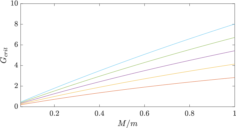
Another revealing quantity is in Eq. 25, where would imply an infinitely large scattering length and hence zero binding energy. In the unitarity limit where the two-body system has a state of zero energy the parameters are constrained by
| (28) |
which combined with Eq. 25 for the -body system leads to the expression
| (29) | ||||
This result is shown in figure Fig. 10 as function of both and . The explicit and reduced mass dependencies explain most of the increases with both and for . The only other quantity is the mean-square-radius of the -body system which decreases and consequently enhances the explicitly increasing factors.
The increase with to far above strongly suggests that at least the energies must change. For a square well, times the critical number (which is for a Gaussian) would correspond to the next infinitely large scattering length. For and we are already halfway to this value where we know that the radius is comparable to the core size, and the state becomes unbound. This means that the scattering length corresponding to the unequal particle colliding with the ground state structure of the particles quickly becomes finite and approaching the range of the two-body potential.
It is interesting to note that for , we find values of in the neighborhood of the critical value . This indicates halo structure for these states. In the other end of equal masses, , we might reach the next infinite scattering length corresponding to , that is again a possible halo structure for these states.
VI Conclusion
We have calculated the two lowest-lying weakly bound states of systems of identical bosons, where is between 3 and 8, for different scattering lengths. We use a finite-range Gaussian potential and search for universal structures and limits to applicability of this concept. The range of the potential is used as the unit of length, and the strengths decrease from values corresponding to infinite scattering length to threshold of binding.
The calculated ratios between ground and first excited state energies at the unitarity limit are, due to the finite range, slightly larger than the predicted Efimov scaling factor. The same effect is still present at the thresholds where it is seen in the calculated scattering lengths, also deviating from Efimov scaling predictions. The systematics are in agreement with previous works in the literature for .
We find that two -states accompany each ground state for all at the unitarity limit. When the two-body attraction decreases the bound states move into the continuum one by one while is increasing from . Still both ground and first excited states are found below the ground state of the -body system, until the systematics is broken for . The first excited -body state exceeds the -body ground state when .
Information about the structure of these quantum states can be found in their radii, which monotonically increase with decreasing attraction as the threshold for binding is approached. We find the well established strong divergence of the two-body system and the logarithmic divergence of both states for . In contrast, the radii of the systems approaching zero binding are found to converge towards finite sizes for both the two lowest-lying states for all .
The mean-square-radii of ground and excited states at threshold follow different power law dependences with powers and , at least up to . The structures of the excited states are consistent with two-body halo structures of one particle interacting weakly with the dense -body core. These universal features are broken for as signaled by a radius smaller than the interaction range.
The energies and radii are also calculated for systems where one particle mass is decreased, but only for one interaction with very large scattering length. We find for the ground states that the binding energies increase while the spatial distances decrease as the mass ratio decrease. The identical particles form denser core-structures surrounded by the light particle.
The structures of the first excited states change considerably with decreasing mass ratio. For few particles the core of identical particles is surrounded by the light particle far away. For more than core-particles the light particle is pulled inside the core configuration. These rather peculiar structure variations are due to the relatively strong attraction between all particles in the present calculation. This means in particular that the light particle is subject to a large total attraction from many identical particles. The two-body halo structure is only present for .
In summary, we have found several expected structures, a few a little surprising, some perhaps even strange. We studied identical boson systems from pairwise bound to the thresholds of -body binding. There is clearly a change away from universal structures when the number of particles exceeds . We studied a system with one of the masses decreasing but only with a relatively strong attraction between all particles. The ground state structures change smoothly, while the first excited state structures change rather dramatically with the number of identical particles. This is expected to be different for weaker attraction which is beyond the scope of the present investigation.
Acknowledgements
The authors would like to thank N. T. Zinner for help in devising the project and continuing discussions during its completion as well as a critical reading of the manuscript. This work is supported by the Danish Council for Independent Research.
References
- [1] V. N. Efimov, Phys. Lett. 33B, 563 (1970).
- [2] V. N. Efimov, Sov. J. Nucl. Phys. 12, 589 (1971).
- [3] T. Kraemer, M. Mark, P. Waldburger, J. G. Danzl, C. Chin, B. Engeser, A. D. Lange, K. Pilch, A. Jaakkola, H.-C. Nägerl, et al., Nature 440, 315 (2006).
- [4] M. Zaccanti, B. Deissler, C. D’Errico, M. Fattori, M. Jona-Lasinio, S. Muller, G. Roati, M. Inguscio, and G. Modugno, Nat. Phys. 5, 586 (2009).
- [5] N. Gross, Z. Shotan, S. Kokkelmans, and L. Khaykovich, Phys. Rev. Lett. 103, 163202 (2009).
- [6] S. E. Pollack, D. Dries, and R. G. Hulet, Science 326, 1683 (2009).
- [7] M. Kunitski, S. Zeller, J. Voigtsberger, A. Kalinin, L. P. H. Schmidt, M. Schöffler, A. Czasch, W. Schöllkopf, R. E. Grisenti, T. Jahnke, et al., Science 348, 551 (2015), eprint 1512.02036.
- [8] J. P. D’Incao (2017), eprint arXiv:1705.10860.
- [9] C. H. Greene, P. Giannakeas, and J. Pérez-Ríos (2017), eprint arXiv:1704.02029.
- [10] P. Naidon and S. Endo, Reports on Progress in Physics 80, 056001 (2017).
- [11] R. D. Amado and F. C. Greenwood, Phys. Rev. D 7, 2517 (1973).
- [12] H.-W. Hammer and L. Platter, Eur. Phys. J. A 32, 113 (2007).
- [13] J. von Stecher, J. P. D’Incao, and C. H. Greene, Nat. Phys. 5, 417 (2009).
- [14] F. Ferlaino, S. Knoop, M. Berninger, W. Harm, J. P. D’Incao, H.-C. Nägerl, and R. Grimm, Phys. Rev. Lett. 102, 140401 (2009).
- [15] I. V. Brodsky, M. Y. Kagan, A. V. Klaptsov, R. Combescot, and X. Leyronas, Phys. Rev. A 73, 032724 (2006).
- [16] M. Thøgersen, D. V. Fedorov, and A. S. Jensen, EPL (Europhysics Letters) 83, 30012 (2008), eprint 0806.3839.
- [17] A. Deltuva, Phys. Rev. A 82, 040701 (2010), eprint 1009.1295.
- [18] J. von Stecher, J. Phys. B: At. Mol. Opt. Phys. 43, 101002 (2010).
- [19] J. von Stecher, Phys. Rev. Lett. 107, 200402 (2011).
- [20] A. Deltuva, Phys. Rev. A 85, 042705 (2012), eprint 1203.6291.
- [21] M. Gattobigio, A. Kievsky, and M. Viviani, Phys. Rev. A 86, 042513 (2012).
- [22] B. Bazak, M. Eliyahu, and U. van Kolck, Phys. Rev. A 94, 052502 (2016).
- [23] Y. Horinouchi and M. Ueda, Phys. Rev. A 94, 050702 (2016), eprint 1603.05328.
- [24] A. Kievsky, M. Viviani, R. Álvarez-Rodríguez, M. Gattobigio, and A. Deltuva, Few-Body Systems 58, 66 (2017), eprint 1702.06465.
- [25] A. Zenesini, B. Huang, M. Berninger, S. Besler, H.-C. Nägerl, F. Ferlaino, R. Grimm, C. H. Greene, and J. von Stecher, New J. Phys. 15, 043040 (2013).
- [26] D. Blume and Y. Yan, Phys. Rev. Lett. 113, 213201 (2014).
- [27] V. Efimov, Nucl. Phys. A 210, 157 (1973).
- [28] G. Barontini, C. Weber, F. Rabatti, J. Catani, G. Thalhammer, M. Inguscio, and F. Minardi, Phys. Rev. Lett. 103, 043201 (2009).
- [29] R. Pires, J. Ulmanis, S. Häfner, M. Repp, A. Arias, E. D. Kuhnle, and M. Weidemüller, Phys. Rev. Lett. 112, 250404 (2014).
- [30] S.-K. Tung, K. Jiménez-García, J. Johansen, C. V. Parker, and C. Chin, Phys. Rev. Lett. 113, 240402 (2014).
- [31] R. S. Bloom, M.-G. Hu, T. D. Cumby, and D. S. Jin, Physical Review Letters 111, 105301 (2013), eprint 1304.6989.
- [32] R. A. W. Maier, M. Eisele, E. Tiemann, and C. Zimmermann, Physical Review Letters 115, 043201 (2015).
- [33] J. Ulmanis, S. Häfner, R. Pires, E. D. Kuhnle, M. Weidemüller, and E. Tiemann, New Journal of Physics 17, 055009 (2015).
- [34] J. Ulmanis, S. Häfner, R. Pires, F. Werner, D. S. Petrov, E. D. Kuhnle, and M. Weidemüller, Phys. Rev. A 93, 022707 (2016).
- [35] L. J. Wacker, N. B. Jørgensen, D. Birkmose, N. Winter, M. Mikkelsen, J. Sherson, N. Zinner, and J. J. Arlt, Physical Review Letters 117, 163201 (2016), eprint 1604.03693.
- [36] J. Johansen, B. J. DeSalvo, K. Patel, and C. Chin, ArXiv e-prints (2016), eprint 1612.05169.
- [37] J. P. D’Incao and B. D. Esry, Phys. Rev. A 73, 030703 (2006).
- [38] K. Helfrich, H.-W. Hammer, and D. S. Petrov, Phys. Rev. A 81, 042715 (2010), eprint 1001.4371.
- [39] Y. Wang, J. Wang, J. P. D’Incao, and C. H. Greene, Phys. Rev. Lett. 109, 243201 (2012).
- [40] M. Mikkelsen, A. S. Jensen, D. V. Fedorov, and N. T. Zinner, Journal of Physics B Atomic Molecular Physics 48, 085301 (2015), eprint 1501.05137.
- [41] D. S. Petrov and F. Werner, Phys. Rev. A 92, 022704 (2015), eprint 1502.04092.
- [42] D. V. Fedorov, M. Mikkelsen, A. S. Jensen, and N. T. Zinner, Few-Body Systems 56, 889 (2015), eprint 1503.04024.
- [43] J. Levinsen, N. R. Cooper, and V. Gurarie, Phys. Rev. A 78, 063616 (2008), eprint 0808.1304.
- [44] Y. Nishida, S. Moroz, and D. T. Son, Physical Review Letters 110, 235301 (2013), eprint 1301.4473.
- [45] A. G. Volosniev, D. V. Fedorov, A. S. Jensen, and N. T. Zinner, Journal of Physics B Atomic Molecular Physics 47, 185302 (2014), eprint 1312.6535.
- [46] S. Moroz and Y. Nishida, Phys. Rev. A 90, 063631 (2014), eprint 1407.7664.
- [47] M. A. Efremov and W. P. Schleich, ArXiv e-prints (2014), eprint 1407.3352.
- [48] D. K. Gridnev, Journal of Physics A Mathematical General 47, 505204 (2014).
- [49] C. Gao, J. Wang, and Z. Yu, Phys. Rev. A 92, 020504 (2015), eprint 1412.3566.
- [50] S. Deng, Z.-Y. Shi, P. Diao, Q. Yu, H. Zhai, R. Qi, and H. Wu, Science 353, 371 (2016), eprint 1512.02044.
- [51] C. H. Schmickler, H.-W. Hammer, and E. Hiyama (2017), eprint arXiv:1703.01147.
- [52] M. Thøgersen, D. V. Fedorov, A. S. Jensen, B. D. Esry, and Y. Wang, Phys. Rev. A 80, 013608 (2009), eprint 0909.4649.
- [53] P. K. Sørensen, D. V. Fedorov, A. S. Jensen, and N. T. Zinner, Journal of Physics B Atomic Molecular Physics 46, 075301 (2013a), eprint 1212.1398.
- [54] M. Berninger, A. Zenesini, B. Huang, W. Harm, H.-C. Nägerl, F. Ferlaino, R. Grimm, P. S. Julienne, and J. M. Hutson, Physical Review Letters 107, 120401 (2011), eprint 1106.3933.
- [55] C. Chin, ArXiv e-prints (2011), eprint 1111.1484.
- [56] R. Schmidt, S. P. Rath, and W. Zwerger, European Physical Journal B 85, 386 (2012), eprint 1201.4310.
- [57] P. Naidon, E. Hiyama, and M. Ueda, Phys. Rev. A 86, 012502 (2012), eprint 1109.5807.
- [58] J. Wang, J. P. D’Incao, B. D. Esry, and C. H. Greene, Physical Review Letters 108, 263001 (2012), eprint 1201.1176.
- [59] P. K. Sørensen, D. V. Fedorov, A. S. Jensen, and N. T. Zinner, Phys. Rev. A 86, 052516 (2012), eprint 1206.2274.
- [60] P. K. Sørensen, D. V. Fedorov, A. S. Jensen, and N. T. Zinner, Phys. Rev. A 88, 042518 (2013b), eprint 1307.2854.
- [61] J. P. D’Incao, J. Wang, B. D. Esry, and C. H. Greene, Few-Body Systems 54, 1523 (2013), eprint 1211.7357.
- [62] S. Roy, M. Landini, A. Trenkwalder, G. Semeghini, G. Spagnolli, A. Simoni, M. Fattori, M. Inguscio, and G. Modugno, Physical Review Letters 111, 053202 (2013), eprint 1303.3843.
- [63] P. Naidon, S. Endo, and M. Ueda, Physical Review Letters 112, 105301 (2014), eprint 1403.0294.
- [64] E. Hiyama and M. Kamimura, Phys. Rev. A 90, 052514 (2014), eprint 1409.2501.
- [65] Y. Horinouchi and M. Ueda, Physical Review Letters 114, 025301 (2015), eprint 1409.3294.
- [66] Y. Suzuki and K. Varga, Stochastic Variational Approach to Quantum-Mechanical Few-Body Problems (Springer, 1998).
- [67] B. Silvestre-Brac and V. Mathieu, Phys. Rev. E 76 (2007).
- [68] M. Gattobigio and A. Kievsky, Phys. Rev. A 90, 012502 (2014),
- [69] L. Platter, H.-W. Hammer, and U.-G. Meißner, Phys. Rev. A 70, 052101 (2004).
- [70] A. Deltuva, Few-Body Syst. 54, 569 (2013).
- [71] A. S. Jensen, K. Riisager, D. V. Fedorov, and E. Garrido, Rev. Mod. Phys. 76, 215 (2004).
- [72] D. V. Fedorov, A. S. Jensen, and K. Riisager, Phys. Rev. C 50, 2372 (1994).
- [73] M. T. Yamashita, D. V. Fedorov, and A. S. Jensen, Few-Body Syst. 51, 135 (2011).