Selective inference after likelihood- or test-based model selection in linear models
Abstract
Statistical inference after model selection requires an inference framework that takes the selection into account in order to be valid. Following recent work on selective inference, we derive analytical expressions for inference after likelihood- or test-based model selection for linear models.
Keywords:
AIC; likelihood-based model selection; linear models; selective inference; test-based model selection1 Introduction
The invalidity of standard inference after model selection has been mentioned by many authors throughout the last decades, including Buehler and Feddersen (1963) and Leeb and Pötscher (2005). Following these publications different approaches for inference in (high-dimensional) regression models after some sort of model selection have emerged over the past years. Initiated by the proposal for valid statistical inference after arbitrary selection procedures by Berk et al. (2013), many new findings and adoptions of post-selection inference (PoSI) to existing statistical methods have been published. Particularly notable is the general framework of Fithian et al. (2014) transferring the classical theory of Lehmann and Scheffé (1955) in exponential family models to selective inference. This post-selection inference concept is based on the conditional distribution of parameter estimators, conditional on the given selection event. Apart from general theory, several authors derive explicit representations of the space to which inference is restricted by well-known selection methods. Initially motivated by the application to the Lasso (Lee et al., 2016, see, e.g.,) several recent publications aim for valid selective inference in forward stepwise regression or any forward stagewise algorithms. In this context, substantial work was done by Tibshirani et al. (2016) as well as by Loftus and Taylor (2014); Loftus and Taylor (2015) for linear models with known error variance . Tibshirani et al. (2016) build a framework for any sequential regression technique resulting in a limitation to the space for inference, where the limitation can be characterized by a polyhedral set. Loftus and Taylor (2014); Loftus and Taylor (2015) extend the idea to a more general framework, for which the limitation of the inference space is given by quadratic inequalities, which coincides with the polyhedral approach in special cases.
Despite the popularity of the Lasso and similar selection techniques in statistical applications, likelihood-based model selection such as stepwise Akaike Information Criterion (Akaike, 1973, AIC,) selection is still used in an extremely vast number of statistical applications and diverse scientific fields (Zhang, 2016, see, e.g.,). However, authors usually do not adjust their inference for model selection, although consequences may be grave (Mundry and Nunn, 2009, see, e.g.,). Selective inference allows to adjust inference after model selection, but an explicit representation of the required conditional distribution for likelihood-based model selection or similar selection procedures has not been derived so far.
We close this gap by explicitely deriving the necessary distribution in linear models with unknown after likelihood- or test-based model selection, which comprises (iterative) model selection based on the AIC or Baysian Information Criterion (Schwarz, 1978, BIC,), model selection via likelihood-based tests, F-tests, and p-value selection (Berk et al., 2013, “significance hunting”,) based on t-tests. We derive an analytical solution for inference in linear models after these model selection procedures and make available an R package for selective inference in such settings in practice (Rügamer, 2017). In addition, we provide inference for multiple and arbitrarily combined selection events, such as stepwise AIC selection followed by significance hunting. We thereby close an important gap in the application of selective inference to model selection approaches that are ubiquitous in statistical applications across all scientific areas.
Section 2 presents the theory on selective testing for linear models and explicitely derives the necessary conditional distributions for several commonly used model selection approaches. In Section 3 we present simulation results for the proposed methods and apply our method to the prostate cancer data. We summarize our concept in Section 4. Derivations of our results and visualizations of additional simulation settings can be found in the supplementary material online.
2 Selective inference in linear models
After outlining the model framework and existing theoretical foundations on selective tests for linear models in Section 2.1, we present the new results on selective tests after various particular selection techniques in Section 2.2 – 2.3. We further show how to extend existing theory for the construction of conditional confidence intervals in Section 2.4 and outline tests of grouped variables in this framework in Section 2.5.
2.1 Setup and theoretical foundation
Given independent variables with true underlying distribution , we consider as possible models submodels of the maximal linear model
for the given data , where are the observed values of and is a fixed design matrix. In particular, we allow the considered models to be misspecified if does not lie in the column space of the design matrix, in which case the corresponding model aims at estimating the linear projection of onto the column space of the design matrix. We then compare two or more linear models based on different column subsets of by using a likelihood-based model selection criterion, as for example the AIC. For the compared subsets, we let with power set function . After selection of the “best fitting” model with design matrix with , we would ideally like to test the th regression coefficient in the set of corresponding coefficients , i.e.
| (1) |
However, taking into account that the true mean is potentially non-linear in the selected covariates or the selection is not correct, we instead test the th component of the projection of into the linear space spanned by the selected covariates :
| (2) |
where is the th unit vector and is the so-called test vector. This coincides with (1) if we select the correct model and is actually linear in . Testing the linear approximation instead of (1) is a more realistic scenario in practice and is in line with the approach of several recent publications including Berk et al. (2013).
We consider the following quadratic inequality introduced in a similar form by Loftus and Taylor (2015), on the basis of which a model is chosen:
| (3) |
before showing that several common model selection approaches lead to restrictions on that can be written in this form. In most practical situations . We are interested in the null distribution of , which we use as a test statistic to test the null hypothesis (2). Since , with under . After model selection of the form (3), conditional on , and also conditional on with the projection of into the space orthogonal to , follows a truncated normal distribution (Loftus and Taylor, 2015) with truncation limits based on , where , and . Due to the form of (3), the two solutions imply that the distribution of our test statistic is truncated to in the case in which is positive, and to if is negative.
2.2 Explicit derivations
We now show that several commonly used model selection approaches can be written as in (3) and explicitely derive the corresponding truncation limits to the normal distribution of the test statistic. For all derivations, please see the supplementary material. We always consider the comparison of two models and in which model is preferred over model . Let be the corresponding covariate subsets of the two considered models and let denote the corresponding design matrix.
Model selection based on log-likelihood comparison plus optional penalty term. We start with conventional model selection procedures that are based on a log-likelihood comparison plus optional penalty term (as, for example, used in the AIC or BIC). Let be the log-likelihood of model and the penalty term for this model, which is assumed not dependent on . For example, if denotes the number of regression coefficients for model and the unknown is estimated, for the AIC and for the BIC. Furthermore, let be the scale parameter estimator and the mean vector estimator of model with and . Then the model is selected iff
| (4) |
with . We therefore define as well as . In the supplementary material we additionally derive the matrix and when treating as known and plugging in , as estimators, i.e. when ignoring the fact that are also functions of , to show the difference.
Model selection on the basis of tests. We first consider the likelihood-ratio test (LRT). For model being nested in model , the derivation is analogous to the AIC comparison by defining , where is the -quantile of the -distribution with degrees of freedom.
The F-Test is not strictly likelihood-based, but falls into the same framework. Let be the residual sum of squares of model . If we choose model , which is nested in model , and denote by the critical value of the F-distribution with and degrees of freedom, then:
| (5) |
where and therefore and . Similarly, if we select the larger model for either LRT or F-test, we simply have to invert the previous inequalities and define as the negative of the respective matrices defined above.
“Significance hunting”. As described in Berk et al. (2013), variable deselection or backward selection on the basis of the size of t-test p-values reduces to deselecting the smallest t-value among several candidates. For the comparison of two variables and and deselection of in the model , it therefore holds that
| (6) |
where and . Let for a given vector . Then (6) is equivalent to and we can define , . If only variables which are not significant are dropped for the “significance hunting”, the t-value of additionally fulfills the condition , where is the quantile function of the Student’s t-distribution with degrees of freedom, which is evaluated with a prespecified significance level to obtain the decision. Since this is equivalent to , we get and .
2.3 Multiple selection events and p-value calculation
If there are selection events of the kind as in Section 2.2, the final space restriction can be calculated by finding the two (or more) most restrictive values in all limiting selection steps. Since this may involve several inequalities with different directions and may result in two or more non-overlapping intervals, additional care is needed. In general, let the resulting truncated normal distribution have multiple truncations given by the ordered intervals , where the case of no finite lower or upper truncation is given by or with intervals or implied by convention, respectively. Let be the observed value of the test statistic, which lies in the interval for some . Then, following Tibshirani.2015, a p-value for the two-sided significance test for (2) based on can be calculated via , with being the p-value of the one sided test. In our setting and as we allow for multiple disjoint truncation intervals, we can define this as , where , and with cumulative distribution function of the standard normal distribution. In other words, is equal to the cumulative probability mass for all possible values that comply with the conditioning event, and is the cumulative probability mass of possible values that are larger than .
As in practice is usually unknown, we investigate in simulations the performance and validity of our proposed p-values when plugging in the restricted maximum likelihood estimate for . We describe the corresponding results in Section 3. Note that while is plugged into the truncated normal conditional distribution for , this distribution is exact and does account for estimation of in the selection event.
2.4 Conditional confidence intervals
We extend the results of Tibshirani et al. (2016) to allow for the construction of selective confidence intervals if the null distribution is truncated to several intervals. We thus find the quantiles and , for which
Analogous to Tibshirani et al. (2016), we can make use of the fact that the truncated normal survival function with multiple truncation limits is also monotonically decreasing in its mean as the truncated normal distribution with multiple truncation intervals is a natural exponential family in (Fithian et al., 2014; Lee et al., 2016, see). The corresponding quantiles can be found via a grid search, where satisfies with being the truncated cumulative normal distribution function with mean , variance and truncation interval(s) . In other words, we search for the mean values and of the truncated normal distribution , for which the observed value is equal to the and quantile, respectively, and thus would not be rejected.
2.5 Testing groups of variables
Following Loftus and Taylor (2015), a selective -significance test for groups of variables can be constructed by testing the null hypothesis where , are the columns of the grouped variable in , is the projection onto the column space of and are the columns of without . Without model selection, a test statistic is given by i.e., follows a -distribution with degrees of freedom under . When conditioning on and the unit vector in the direction of , can be decomposed as , such that the only variation is in . Conditional on the selection event (3), follows a truncated -distribution with truncation limits now given by , and . Depending on the sign of and the number of solutions , the truncation set is either a closed interval , an open interval , or a union of intervals . The test for grouped variables with multiple selection events can be treated analogously to Section 2.3 by normalizing the truncated distribution analogously, replacing with the cumulative distribution function of the -distribution. Note that while the truncated normal distribution is replaced by a truncated -distribution, the types of conditioning events do not change when incorporating groups of variables. The only exception is significance hunting, for which model selection is then not based on t-statistics of regression coefficients but an F-test as in (5) is typically used.
3 Empirical evidence
We evaluate the proposed selective inference concepts in linear models for a forward stepwise selection procedure based on the AIC.
For the simulation study, we consider covariates , observations and use the data generating process respectively correspond to the true active covariates respectively their effects and is Gaussian noise with zero mean and variance , which is determined by the signal-to-noise ratio . Covariates are independently drawn from a standard normal distribution () or exhibit a correlation of (). For each setting, simulation iterations are performed. We present resulting p-values in a uniform quantiles vs. observed p-value-plot in Figure 1, where p-values are calculated on the basis of concepts introduced in Section 2. In the plot, p-values along the diagonal indicate uniformity, which seems to hold for all inactive variables in all given simulation settings. For active variables, the corresponding selective test shows higher power the closer the point line of p-values runs along the axis. Results are based on those simulation iterations in which all of the active covariates and additional inactive covariates are selected. Note that in the selective inference framework, p-values of inactive variables should exhibit uniformity given any particular set of selection events, if the null hypothesis holds. Aggregating across selected models in each panel of Figure 1 results in mixture distributions for the p-values, with a mixture of uniform variables again being . Results for iterations without selected inactive variables (not shown) are similar in terms of power. In summary, p-values for inactive variables exhibit uniformity in every setting. p-values for active covariates indicate large power in most of the settings, with notable exceptions for those simulation settings in which is relatively large in comparison to .
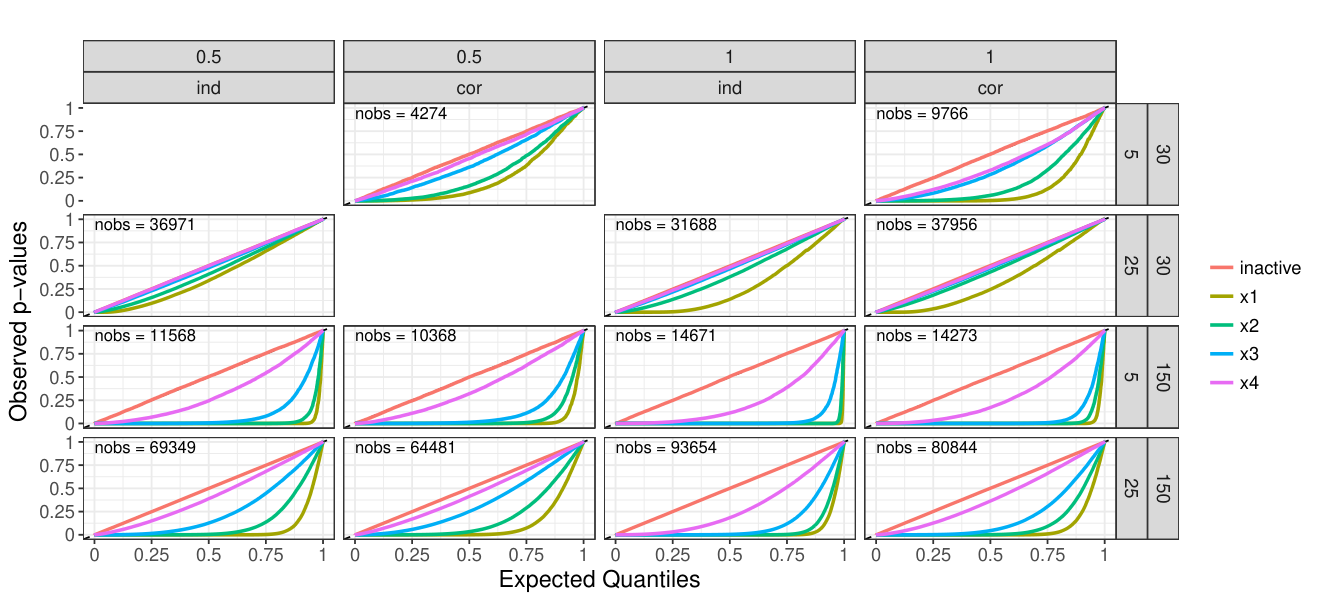
Further results are given in the supplementary material, showing the resulting p-values for simulation iterations in which the selected model is misspecified due to missing active variables and potentially selected inactive variables. Here, p-values of inactive variables exhibit some deviation from the uniform quantiles when not all of the active variables have been selected. However, deviations mainly occur when inactive variables are correlated with unselected active variables in which case the null hypothesis (2) in fact does not exactly hold. This is due to the fact that the linear projection of into the column space of the selected design matrix has a non-zero coefficient for the th variable if a correlated variable is omitted from the model. For the setting with correlation, , and , Table 1 additionally provides the estimated coverage for the confidence intervals constructed as in subsection 2.4, averaging over all iterations where at least all the active variables are selected (and over inactive variables for the inactives column). In addition, we investige the performance of our approach when plugging in for in the derived distribution of for all simulation settings (see supplementary material). p-values for inactive variables still approximately exhibit a uniform distribution when using an estimate for . Notable deviations in comparison to p-values calculated with the true variance can occur when is not estimated well such as for and . Furthermore, as shown in Table 1, almost no difference in the coverage of selective confidence intervals is obtained when plugging in for . In the supplementary material, we also provide results for a simulation study for the -test after stepwise AIC selection with a group noise variable.
| Inactives | |||||
|---|---|---|---|---|---|
| Using true variance | 0.9516 | 0.9492 | 0.9485 | 0.9532 | 0.9542 |
| Using plugin estimate | 0.9496 | 0.9485 | 0.9457 | 0.9515 | 0.9532 |
We additionally apply our approach to the prostate cancer data set (Stamey et al., 1989), which has also been used in Tibshirani et al. (2016) to illustrate selective confidence intervals after forward stepwise regression (see the supplementary material). When using , the significant variables match the two significant variables after forward stepwise regression in Tibshirani et al. (2016), although the selected model is different. Compared to unadjusted inference, confidence intervals become wider for all coefficients in the selective inference framework.
4 Summary
Based on the general selective inference framwork derived in Loftus and Taylor (2014); Tibshirani et al. (2016); Loftus and Taylor (2015), we address the issue of conducting valid inference in linear models after likelihood- or test-based model selection, which comprises (iterative) model selection based on the AIC or BIC, model selection via likelihood-based or F-tests and significance hunting based on t-tests. We explicitely derive the necessary conditional distributions for these selection events, which allows the application of selective inference to additional practically relevant settings compared to existing results. We extend the construction of p-values and confidence intervals to the case in which the distribution of the test statistic conditional on the selection events is truncated to multiple intervals. In simulations, we see that obtained p-values yield desireable properties even if the selected model is not correctly specified and confidence intervals show the nominal coverage. We make available an R software package (Rügamer, 2017) for selective inference to apply the proposed framework in practice.
Acknowledgments
We thank Fabian Scheipl for his useful comments.
References
References
- Akaike (1973) Akaike, H., 1973. Information Theory and an Extension of the Maximum Likelihood Principle. Ed. B. N. Petrov and F. Csaki.
- Berk et al. (2013) Berk, R., Brown, L., Buja, A., Zhang, K., Zhao, L., et al., 2013. Valid post-selection inference. The Annals of Statistics 41, 802–837. doi:10.1214/12-AOS1077.
- Buehler and Feddersen (1963) Buehler, R.J., Feddersen, A.P., 1963. Note on a conditional property of Student’s . Ann. Math. Statist. 34, 1098–1100.
- Fithian et al. (2014) Fithian, W., Sun, D., Taylor, J., 2014. Optimal Inference After Model Selection. ArXiv e-prints arXiv:1410.2597.
- Lee et al. (2016) Lee, J.D., Sun, D.L., Sun, Y., Taylor, J.E., 2016. Exact post-selection inference, with application to the lasso. Ann. Statist. 44, 907–927.
- Leeb and Pötscher (2005) Leeb, H., Pötscher, B.M., 2005. Model selection and inference: facts and fiction. Econometric Theory 21, 21–59.
- Lehmann and Scheffé (1955) Lehmann, E., Scheffé, 1955. Completeness, similar regions, and unbiased estimation: Part ii. The Indian Journal of Statistics 15, 219 – 236.
- Loftus and Taylor (2014) Loftus, J.R., Taylor, J.E., 2014. A significance test for forward stepwise model selection. ArXiv e-prints arXiv:1405.3920.
- Loftus and Taylor (2015) Loftus, J.R., Taylor, J.E., 2015. Selective inference in regression models with groups of variables. ArXiv e-prints arXiv:1511.01478.
- Mundry and Nunn (2009) Mundry, R., Nunn, C., 2009. Stepwise model fitting and statistical inference: Turning noise into signal pollution. The American Naturalist 173, 119–123. PMID: 19049440.
- Rügamer (2017) Rügamer, D., 2017. coinflibs: Conditional Inference after Likelihood-based Selection. URL: https://github.com/davidruegamer/coinflibs. R package version 0.0.0.9000.
- Schwarz (1978) Schwarz, G., 1978. Estimating the dimension of a model. Ann. Statist. 6, 461–464.
- Stamey et al. (1989) Stamey, T., Kabalin, J., McNeal, J., Johnstone, I., Freiha, F., Redwine, E., Yang, N., 1989. Prostate specific antigen in the diagnosis and treatment of adenocarcinoma of the prostate. ii. radical prostatectomy treated patients. The Journal of urology 141, 1076–1083.
- Tibshirani et al. (2016) Tibshirani, R.J., Taylor, J., Lockhart, R., Tibshirani, R., 2016. Exact post-selection inference for sequential regression procedures. Journal of the American Statistical Association 111, 600–620.
- Zhang (2016) Zhang, Z., 2016. Variable selection with stepwise and best subset approaches. Annals of Translational Medicine 4. doi:10.21037/atm.2016.03.35.