Approximate Quantum Error Correction Revisited:
Introducing the Alpha-bit
Abstract
We establish that, in an appropriate limit, qubits of communication should be regarded as composite resources, decomposing cleanly into independent correlation and transmission components. Because qubits of communication can establish ebits of entanglement, qubits are more powerful resources than ebits. We identify a new communications resource, the zero-bit, which is precisely half the gap between them; replacing classical bits by zero-bits makes teleportation asymptotically reversible. This decomposition of a qubit into an ebit and two zero-bits has wide-ranging consequences including applications to state merging, the quantum channel capacity, entanglement distillation, quantum identification and remote state preparation. The source of these results is the theory of approximate quantum error correction. The action of a quantum channel is reversible if and only if no information is leaked to the environment, a characterization that is useful even in approximate form. However, different notions of approximation lead to qualitatively different forms of quantum error correction in the limit of large dimension. We study the effect of a constraint on the dimension of the reference system when considering information leakage. While the resulting condition fails to ensure that the entire input can be corrected, it does ensure that all subspaces of dimension matching that of the reference are correctable. The size of the reference can be characterized by a parameter ; we call the associated resource an -bit. Changing interpolates between standard quantum error correction and quantum identification, a form of equality testing for quantum states. We develop the theory of -bits, including the applications above, and determine the -bit capacity of general quantum channels, finding single-letter formulas for the entanglement-assisted and amortised variants.
1 Introduction
In the theory of quantum information, the most fundamental communications resources are classical bits, qubits and shared entanglement. Those resources are related to each other through interconversion protocols. Teleportation converts an ebit of entanglement11 1 An ebit is another term for a Bell pair of two qubits. plus two classical bits (cbits) of communication into a qubit of communication [1]. Similarly, superdense coding converts a qubit of communication plus an ebit into two classical bits of communication [2]. Those relationships can be thought of as inequalities between resources:
| (1) | ||||
| (2) |
Harrow realised, however, that these inequalities are not tight. He introduced a new communications resource, the coherent bit or cobit, that was intermediate between classical and quantum communication [3]. It could substitute for the cbits in both inequalities, leading to
| (3) | ||||
| (4) |
By cancelling resources on both sides of these inequalities, which corresponds to the catalytic use of resources, Harrow arrived at the identity
| (5) |
That is, the cobit is the arithmetic mean of an ebit and a qubit. This simple insight proved to be a powerful tool for deriving new quantum information protocols from old. (For a version of the argument without catalysis, see [4, 5].)
In this article, we will continue in this tradition by introducing new communications resources, -bits, that upgrade other fundamental resource inequalities into identities. As will be described in more detail below, these -bits correspond to the ability to perform quantum error correction on arbitrary bounded-dimension subspaces, with the real number characterizing the size of the subspace. The case is standard quantum error correction, while is closely related to quantum identification, a form of equality testing for quantum states.
It is a trivial consequence of their definitions that qubits are stronger than cobits are stronger than ebits:
| (6) |
We show that the gap in each inequality is precisely a zero-bit. That is,
| (7) |
as illustrated in Figure 1.

Harrow’s identity is then an immediate consequence. More interestingly, these identities establish that both cobits and qubits are composite resources, decomposable in terms of weaker constituents asymptotically.
Combining the two identities of (7) yields a new form of teleportation with zero-bits substituting for classical bits:
| (8) |
with the inequality of (1) now an identity. This identity decomposes qubit communication into a pure correlation part, the ebit, and a pure communication part, the zero-bits. Unlike when one substitutes cobits for cbits in teleportation, zero-bit-powered teleportation achieves qubit transmission and nothing else. In this sense, zero-bits are the minimal and thus most natural communications resource for teleportation. Moreover, by using resources catalytically to cancel (8) against (1), we find that zero-bits are weaker than cbits despite being quantum resources.
These conclusions are corollaries to the general theory of -bits, which in turn arise as natural tools for studying approximate quantum error correction [6]. Relaxing the conditions of quantum error correction from exact [7, 8] to approximate has long been known to yield surprising improvements [9]. One of the most striking examples is that, while exact quantum error correcting codes can arbitrary errors on at most of the system at a time, approximate codes can correct errors on up to of the system even for vanishingly small errors (with sufficiently large systems) [10]. The capacity of a channel to send qubits, its quantum capacity [11], itself relies crucially on being allowed to make very small errors. If one requires absolute perfection then the resulting capacity is typically smaller, usually zero [12]. Of course, once one allows for the possibility of small errors, it becomes necessary to quantify those errors. Different reasonable definitions have, until now, all proven to be closely related to each other. Indeed, a wide variety of slightly different notions of quantum capacity are all known to be equal to each other [13]. The focus of this article, however, will be on a form of approximate quantum error correction which is asymptotically distinct from the usual one.
Because the definitions involved are quite technical, we will begin by illustrating the basic phenomenon we are trying to capture with a relatively simple example: a channel induced by a Haar-random unitary transformation. Suppose we apply such a unitary to some large number of qubits then throw away a fraction that is slightly less than half. Call the input Hilbert space , the qubits that are kept and the qubits that are discarded . Now consider the fate of a typical pair of orthogonal pure states on in the limit of large . Both will get mapped to states almost maximally entangled between and . Moreover, because is much smaller than , the reduced states on will be nearly maximally mixed and therefore effectively indistinguishable. For the same reason, the states on will have small rank relative to the dimension of , which leads to their being nearly orthogonal.
In fact, due to strong measure concentration effects in high dimension, those properties will hold not just for one pair of orthogonal states on , or two pairs, or even a countable number of pairs. It will hold for all pairs of orthogonal states in a subspace of that is almost as large as in qubit terms: qubits. More generally, the map from to approximately preserves the pairwise distinguishability of states as measured by the trace distance despite shrinking the number of qubits by a factor of two [14, 15]. Because the dimension of the state space of is roughly the square root of that of , that would seem to be a paradox. The resolution is that the map encodes some of the geometry of the unit sphere into the eigenvalues of the state on ; pure state geometry is partially encoded into noise. At this point, we could simply define “sending the zero-bits of ” to mean approximately preserving the geometry of the unit sphere. The actual definition is slightly more complicated but also more useful and more generalisable.
Returning to the example, while the full subspace has been transmitted in some sense, it is clearly not possible to perform approximate quantum error correction and completely reverse the effect of the channel; doing so would lead to the quantum capacity of a qubit being greater than one, which by recursion would mean it was infinite. Geometry preservation does have an operational consequence, however. If we restrict the states to any two-dimensional subspace of , then there is a decoding operation that will perform quantum error correction. The only catch is that the decoding operation will depend on the two-dimensional subspace in general. Note, however, that the encoding and the channel do not. If we think of Alice sending Bob a state, then Bob must know which two-dimensional subspace the state is in while Alice does not.
What if Bob wishes to be able to decode larger subspaces of ? What fraction of the qubits do they then need to keep? To decode the entire space requires that essentially all the qubits be kept. It turns out that if they keep a fraction greater than of the qubits then he can decode any subspace of up to qubits.22 2 Technically, our construction requires the use of shared randomness to achieve this rate but it can be eliminated by block coding. We call this task universal approximate subspace error correction and say that contains the -bits of . As before, the number of -bits is determined by the dimension of rather than the dimension of the subspaces Bob wishes to decode because the whole space is available to him; he just needs to make a choice about which subspace he is interested in. A zero-bit is then simply the special case of an -bit with .
Quantum geometry preservation was studied in [15], together with the very closely related task of quantum identification [14, 20]. General universal subspace error correction is then the natural interpolation between the geometry preservation limit, where the subspaces are two-dimensional, and ordinary approximate quantum error correction, where the subspace is the complete space.
We are now ready to turn to the general formalism of -bits and universal approximate subspace error correction. Let denote the set of density operators acting on Hilbert space . Approximate quantum error correction in the usual sense is defined for a quantum channel , defined to be a completely positive, trace-preserving map [16], by the existence of a decoding channel such that
| (9) |
The Hilbert space here is a reference system with which the space may be entangled. The capacity of a channel to send quantum information defined in this sense has long been understood to be the regularized maximum coherent information between the output of the channel and the reference system with which the input was entangled [17, 18, 19].
Universal approximate subspace error correction is an easier task, since the receiver is only required to be able to decode states in any subspace of their choice, up to some fixed maximum dimension . In the limit of an asymptotically large Hilbert space, this task is inequivalent to standard approximate quantum error correction. This leads to surprising consequences. As we have already seen, a noiseless qubit channel can carry more than one qubit’s worth of information if we only need to be able to decode small subspaces. Meanwhile, a noiseless classical bit channel, which one would expect should be useless for quantum error correction, can have an (amortised) capacity which is strictly positive.
For any quantum channel, the Stinespring dilation theorem [21] states that there exists an ancilla space and isometry such that for all density matrices
| (10) |
Since is uniquely defined up to isomorphisms, it follows that the so-called complementary channel , defined as
| (11) |
is also unique up to isomorphisms. A key insight in understanding quantum error correction [6, 22, 19, 23] is that approximate error correction is possible if and only if the complementary channel is approximately completely forgetful. To make this notion more precise, we first define the -diamond norm.
Definition 1 (-diamond norm).
For a linear superoperator , the -diamond norm is defined by
where the maximisation is over operators on . The diamond norm, also known as the completely bounded trace norm, is then defined as
Because of the convexity of the trace norm, this supremum is always achieved on a rank-one operator (a pure quantum state in the case of a Hermiticity-preserving superoperator). Since any state in can be purified by a reference system of dimension at most the dimension of , the diamond norm is identical to the -diamond norm.
Definition 2 (-forgetfulness).
We say that a channel is approximately -forgetful if
where is the channel taking all states to for the maximally mixed state in .
The case of is referred to simply as approximate forgetfulness, while the case of , where the norm is the actual diamond norm is known as complete forgetfulness. For convenience, we will also refer to -forgetfulness, where is the dimension of the Hilbert space, simply as -forgetfulness.
As stated above, approximate quantum error correction in the sense of (9) is equivalent to complete forgetfulness with a universal relation (independent of system size) between and . (See, e.g., [24].) Moreover, in exactly the same way, approximate forgetfulness was found to be equivalent to geometry preservation [15], a result known as the weak decoupling duality. To begin to see why these notions of error correction are not equivalent, note that the tightest achievable bound on the diamond norm in terms of the 1-diamond norm is [25]
| (12) |
As a result, approximate geometry preservation to any fixed level of precision is not sufficient to usefully bound the error in decoding the entire space as . In sharp contrast, it should also be evident that exact geometry preservation (and hence universal subspace error correction) does imply exact quantum error correction. The two decoupling results turn out to have exactly the interpolation one would expect; we shall prove in Section 2 that universal subspace error correction is equivalent to -forgetfulness, where is the maximum dimension of the subspaces we wish to be able to decode.
In Section 3 we exploit this equivalence to develop a central result of the paper: a formula for the capacity of a quantum channel to send sufficient information for universal subspace error correction. As we saw above for a noiseless channel, this turns out to be a function of a parameter , where, if is the dimension of the Hilbert space and is the dimension of the subspace we want to measure,
| (13) |
We refer to the resulting capacity as the -bit capacity of the channel. The theorem validates the definition of universal subspace quantum error correction by demonstrating that designing codes specifically tailored to a given size of subspace increases the transmission rate.
The general form of the -bit capacity is somewhat complicated, but with either of two possible relaxations it simplifies to the single letter formula
where is the channel mutual information. The first relaxation is to give the two parties shared entanglement as a free resource - the entanglement-assisted capacity. The second possibility is to consider the amortised capacity of the channel, which is the incremental -bit capacity supplied by the channel in the presence of an arbitrarily large noiseless quantum side channel. Although the first of these will probably be more familiar to readers well acquainted with standard results about quantum capacities, in both cases the effect is simply to provide an additional source of coherence between the two parties. The amortised capacity is less studied because, as , the size of the side channel required becomes infinite, and so finite noiseless side channels are of no use in standard error correction. The entanglement-assisted capacity, on the other hand, has the expected limit as , namely the entanglement-assisted quantum capacity. If we take , however, it becomes equal to the entanglement-assisted classical capacity. This second equality was noted in [15] but was regarded there as a puzzling coincidence.
In Section 4 we explore how -bits can be used. Our first result is that combining -bit transmission with shared entanglement is enough to send classical information at a rate of cbits per -bit, providing an operational explanation for the coincidence described above. We then extend the argument to the case where entanglement is a limited resource by making use of the notion coherent classical bits, or cobits. We find that the identity
| (14) |
generalises to -bits as
| (15) |
The identities involving zero-bits described at the start of the introduction are immediate consequences of these relations.
Section 4 also derives a number of consequences from these identities. We find that zero-bits can substitute for classical bits in a wide variety of circumstances including teleportation, state merging, entanglement distillation, channel simulation and remote state preparation. We also strengthen the previously mentioned coherent information lower bound on the quantum capacity of a quantum channel, demonstrating that in addition to sending qubits at the coherent information rate, it is possible to simultaneously send zero-bits at a rate given by the mutual information with the environment.
The detailed proof of the -bit capacity theorem appears in Section 5. Section 6 proves some important supplementary results, including an alternate characterisation of the -bit capacity and a single-letter formula for degradable channels. The -bit capacities of two simple quantum channels are studied as examples in Section 7. A summary of our main results appears in Section 8. The paper ends in Section 9 with an argument that zero-bits and ebits should be regarded as the fundamental resources of quantum information, as well as speculations on how to extend the paradigm to classical communication.
2 Decoupling and universal subspace error correction
We first prove the duality between -forgetfulness and universal subspace error correction. Our starting point is a well-known information-disturbance theorem.
Theorem 1 (Information-Disturbance [23]).
Let be an isometric extension of the channel and let be the complementary channel. Let be the channel taking all inputs to some fixed state . Then
| (16) |
The infimums are over all quantum channels.
As discussed in the introduction, the diamond norm is equivalent to the -diamond norm for any Hilbert space of dimension . Furthermore by the convexity of the trace norm, the -diamond norm for a superoperator on is attained by a pure state on , which necessarily has support only within some -dimensional subspace of . It is therefore clear that, for acting on ,
| (17) |
where is the restriction of to acting on for any subspace of dimension less than or equal to . We can then arrive at the following theorem as a relatively simple consequence of the information-disturbance theorem
Theorem 2 (Subspace Decoupling Duality).
Suppose we have a channel such that the complementary channel is -forgetful, i.e.
| (18) |
where takes all states to for some fixed state . Then for any subspace of dimension less than or equal to , there exists a decoding channel such that
| (19) |
where is the restriction of to .
Conversely, if for all subspaces of dimension less than there exists a decoding channel such that
| (20) |
then
| (21) |
where takes all states to for some .
Proof.
Starting from -forgetfulness, let us first choose a fixed subspace of dimension less than or equal to . From (18), we know that for any state
| (22) |
It follows from the triangle inequality that for all states
| (23) |
Defining as the restriction of to and as the channel taking all states to , we therefore find that
| (24) |
and hence by Theorem 1 there exists a decoding channel such that
| (25) |
To prove the converse, we first fix a pure state . Let be a -dimensional subspace containing and let be the restriction to of . Then by Theorem 1 there exists taking all states to some fixed state such that for any state
| (26) |
If is the channel taking all states to then by the triangle inequality
| (27) |
If we now take , then for any pure state we can choose such that and hence (27) is true. It follows by the convexity of the trace norm that
| (28) |
and hence using (12) that
| (29) |
which completes the proof. ∎
3 Alpha-bits and capacities
3.1 Alpha-bits
We are interested in the capacity of quantum channels to transmit information about large Hilbert spaces in order to achieve universal subspace error correction for subspaces of some defined size. As we have seen in Section 2, up to universal relations in the size of the error, universal subspace error correction for all fixed finite subspace sizes is equivalent to error correction for subspaces of dimension 2 (i.e. geometry preservation), which is well-understood. Similarly, when the subspace size is a fixed finite fraction of the entire space, universal subspace error correction is equivalent to ordinary quantum error correction.
The regime that still needs to be understood then is when the subspaces grow sublinearly a function of the dimension of the Hilbert space. A natural choice is for the subspaces to have maximum dimension for . This leads to a channel capacity that depends only on and naturally interpolates between the geometry preservation and quantum capacities. Since this interpolation is continuous,33 3 As proved in Lemma 12, the -bit capacity is a continuous function of , as is the entanglement-assisted -bit capacity. However, the amortised -bit capacity has a discontinuity at . As a result, it remains an open question to find and prove amortised universal subspace error correction capacities for subspace dimensions that grow sublinearly but faster than for any . this capacity is sufficient to determine the capacity for any sublinear simply by defining
In fact, we shall need to very slightly modify the requirement in order to handle . In that case, the subspaces are dimensional, so decoding them is always trivial. Instead, we wish for to correspond to decoding two-dimensional subspaces. (Any constant dimension two or larger is equivalent.) We shall therefore require that it be possible to decode all subspaces of dimension less than or equal to rather than . Since the decoding error grows at most linearly with the size of the subspace, the only effect of this change is to redefine the decoding error by at most a factor of two. Since we are only interested in whether the error tends to zero in certain limits, and are completely equivalent for our purposes for while using properly incorporates the case .
We therefore make the following definition.
Definition 3 (-dit).
Let Alice have a qudit in Hilbert space of dimension . We say that she is able to transmit her state to Bob through as an -dit with error if, for any subspace of with dimension less than or equal to , there exists a decoding channel such that for all states
| (30) |
where is the encoding used by Alice for .
Since the error grows at most linearly with the size of the subspace that must be decoded, we will need to take the limit of large for -dits to become sharply defined and for -dits with different values of not to be equivalent up to small rescalings in the allowed error . It is therefore necessary to define a normalisation of an -dit that is well-behaved as . This leads us naturally to a second definition.
Definition 4 (-bit [Informal]).
Informally, we define an -bit to be
We wil define an -bit more precisely in the specific contexts that we use the term and so we shall not attempt to provide a more formal definition here. It is of course unclear exactly what a limit means in this context; the basic intuition is that we shall require properties to hold for all sufficiently large for any fixed and sufficiently small . In general, the minimum size of the dimension will tend to infinity as the error tends to zero.
It is important to note that an -bit is emphatically not the same as a single -dit with . This might potentially be regarded as misleading given the relationship between qubits and qudits. However, it is hoped that in practice it should be clear, since in the case of an -dit is exactly equivalent to a noisy qubit and importantly has absolutely no dependence on . An -bit defined as an -dit with would therefore be a completely redundant notion.
Definition 5 (Total error).
If Alice transmits -dits with errors , we define the total error .
This definition will prove useful when we come to define the -bit capacity. We motivate its definition with the following lemma.
Lemma 3.
Let , where the index parameterises a set of -dits, all have dimension less than or equal to and have decoding channel with error less than or equal to as in Definition 3. Then for all states
| (31) |
Proof.
Since we are restricting to a specific set of error-correctable subspaces, this is just a question about ordinary quantum error correction. We define
where acts as the identity on all subsystems that are not listed. Then by the triangle inequality
| (32) |
However, and for any state , we have so
| (33) |
∎
3.2 Capacities
We are now ready to define the notion of an -bit capacity of a quantum channel.
Definition 6 (-bit capacity).
We say that a rate of -bit transmission through a channel is achievable if, for all as well as sufficiently large and , it is possible to transmit
with total error using the channel . The -bit capacity of is then defined as the supremum over achievable rates.
Definition 6 is not the only possible definition of the -bit capacity of a channel. Another fairly natural and slightly stricter definition of the achievability of a rate gives what we shall refer to as the single -dit capacity of the channel.
Definition 7 (Single -dit capacity).
We say that a rate of single -dit transmission through a channel is achievable if for all as well as sufficiently large it is possible to transmit an -dit with dimension
with error using the channel . The single -dit capacity of is then defined as the supremum over achievable rates.
Note that the single -dit capacity is still normalised in terms of -bits. However, the -bits are only allowed to form a single -dit, rather than arbitrarily many -dits. It is clear that if single -dit transmission at rate is achievable then the same rate is achievable for -bit transmission and hence optimality of a given capacity for -bit transmission implies optimality of the same capacity for single -dit transmission. On the other hand achievability of a single -dit transmission rate does not follow from achievability of the same rate for -bit transmission. Our construction does achieve a single -dit capacity equal to the -bit capacity, but only by making catalytic use of a large amount of shared randomness.
The -bit capacity is in many ways the more natural quantity to consider, particularly in the context of the resource inequality framework explored in Section 4. If you sent -dits and subsequently sent another -dits, then you have sent -dits, just like for cbits or qubits. In contrast, sending an -dit with followed by an -dit with does not mean that you have sent an -dit with .
As a trivial counterexample, let and . If sending two -dits was equivalent to sending one -dit with dimension then if Alice sent a state that is known by Bob as the second -dit, Bob would be able to decode a state of dimension on the joint system and would be guaranteed to be able to decode the first state he received. Clearly this is impossible without Bob being able to do full error-correction rather than just universal subspace error correction.
We shall also formally define two further variants of the -bit capacity, which turn out to have a particularly simple form. To define the amortised -bit capacity we need to first introduce a noiseless quantum side channel . The amortised capacity of a channel is the increase in capacity from having the channel as well as the side channel , rather than just the side channel. We shall see in Theorem 4 that the -bit capacity of a noiseless qudit channel is
This leads to the following technical definition for the amortised -bit capacity.
Definition 8 (Amortised -bit capacity).
We say that a rate of amortised -bit transmission through a channel is achievable if, for all as well as sufficiently large and , it is possible to transmit at least
with total error using the channel where the noiseless quantum side channel may have any size. The amortised -bit capacity of is then defined as the supremum over achievable rates.
Finally, we define the entanglement-assisted -bit capacity. The definition is analogous to the definitions of entanglement-assisted quantum or classical capacities.
Definition 9 (Entanglement-assisted -bit capacity).
We say that a rate of entanglement-assisted -bit transmission through a channel is achievable if, for all as well as sufficiently large and , it is possible to transmit at least
with total error using the channel and a shared maximally entangled state of unlimited size. The entanglement-assisted -bit capacity of is then defined as the supremum over achievable rates.
While the entanglement-assisted -bit capacity is defined analogously to the -bit capacity for consistency, our achievability proof actually yields the stronger single -dit transmission in the entanglement-assisted setting.
As with essentially all types of channel capacity, the -bit capacity is characterized most succintly in terms of entropies of reduced density matrices. For a bipartite density matrix we define the von Neumann entropy of
The mutual information of the state is
while the coherent information is
Theorem 4 (-bit capacity).
The -bit capacity of a channel is given by
| (34) |
where
| (35) |
for and
| (36) |
is a purification of any input state of the channel and we define . The amortised -bit capacity (for ) and the entanglement-assisted capacity are both given by
| (37) |
Theorem 4 generalises both the quantum capacity formula of [17, 18, 19] (when ) and the quantum identification capacity formula of [15] (when ). Since the zero-bit capacity will play a special role in our discussion, it is worth noting that [15] demonstrates that it is possible to achieve the single zero-dit capacity at the rate above, not just the slightly easier zero-bit capacity.
One of the most striking features of the theorem is that the amortised -bit capacity is positive for all non-trivial channels, even those that are purely classical. This is true even for arbitrarily close to one, for which success translates to being able to quantum error correct arbitrary subspaces of the input with fractional size approaching one (as measured in qubits). -bit codes for can therefore be used as quantum data transmission codes: transmission of -bits implies the transmission of qubits. This would suggest that the amortised quantum capacity should be equal to
| (38) |
the entanglement-assisted quantum capacity. Sadly, this is not the case. In the definition of the amortised -bit capacity, one subtracts from the total number of -bits transmitted the number that could have been transmitted by the noiseless side channel:
| (39) |
for a side channel of dimension . As applied to quantum data transmission, that corresponds to subtracting
| (40) |
from the total number of qubits transmitted. But the noiseless side channel could actually transmit qubits, which is strictly larger than (40), so the subtraction fails to account for the full strength of the side channel applied to quantum data transmission. Since the prefactor in (40) satisfies
| (41) |
one might hope that the incorrect accounting would correct itself in the limit . However, it turns out that the size of the side channel, , depends on and even diverges superlinearly with as , ensuring that (38) is, in general, not the correct formula for the amortised quantum capacity. It is nonetheless instructive to see how, from the -bit perspective, the difficulty of finding a single-letter formula for the (amortised) quantum capacity arises from singular behavior at .
Here, we will only explain the basic construction used to prove Theorem 4, postponing the somewhat technical detailed proof to Section 5. The structure of the -bit code that we will use to achieve the capacity is given in Figure 2. The encoding channel (with Stinespring dilation ) that we will use consists of a unitary map from input space to where is a typical subspace of for some large number of channel uses and is an auxiliary Hilbert space which will be thrown away. We apply a unitary operator selected at random and known by both Alice and Bob from a unitary 2-design and then trace out .
We are then able to prove that the complementary channel will be -forgetful (and so by Theorem 2 we can use the channel to transmit -dits) so long as the effective size of the environment and reference is much smaller than the effective size of the Hilbert space transmitted to Bob. To make this more precise, we define as a Stinespring dilation of and choose some pure state , using which we will construct the typical subspace . Then, in the limit of large we require that
| (42) |
where and .
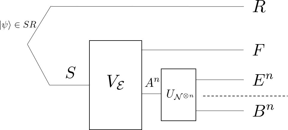
The size of the code space is bounded by the total size of the typical subspace of and . This gives a second constraint
| (43) |
Combining these inequalities, we find that
| (44) | |||
| (45) |
If we can find such that both the original inequalities (42) and (43) can be simultaneously satisfied, then the corresponding rate will be achievable. Unfortunately this is not possible in general, because our construction only allows . This means that (42) imposes the further constraint that a rate is only achievable if
| (46) |
Note that we were under no obligation to only have one channel use in the definition of the state . If we optimise over the number of channel uses that are used to construct , we obtain the -bit capacity given in Theorem 4.
We shall see in Section 5 that either amortisation or entanglement-assistance removes the effect of the restriction that . For example, by using approximately
we are able to ensure that the effective size of the environment is much smaller than the effective size of Bob’s Hilbert space simply by sending not only the code space using the protocol given in Figure 2, but also Alice’s half of the Bell pairs. The cost is that this reduces the size of the code space that can be transmitted with , giving a new constraint
| (47) |
or
| (48) |
Furthermore, the optimised mutual information is additive [26], unlike the coherent information. As a result,we do not need to consider the optimising over multiple channel uses and we are left with the simple single letter formula given in Theorem 4.
The only remaining challenge is to generate a sufficient supply of shared randomness between Alice and Bob to be able select randomly from a unitary 2-design. We will show that this can be seeded through the channel at arbitrarily small cost to the asymptotic rate.
4 Alpha-bits as resources
4.1 Entanglement-assisted classical capacity of an -bit
When , the entanglement-assisted -bit capacity of a channel given in Section 3 is equal to the entanglement-assisted classical capacity. This equality was noticed (for the amortised rather than entanglement-assisted) capacity in [15] and was regarded as a puzzle. It turns out to have a very natural explanation; an -bit code for a channel achieving the entanglement-assisted -bit capacity can always be used directly together with additional free entanglement to achieve the entanglement-assisted classical capacity of the channel.
Definition 10 (Entanglement-assisted classical capacity of an -bit).
We say that an
entanglement-assisted classical transmission rate is achievable using -bits if, for all , there exists , such that for all sufficiently large , it is possible to transmit bits of classical information with error probability at most , using an -dit with error and free shared entanglement. Furthermore, we require that if , then .
The entanglement-assisted classical capacity of an -bit is defined as the supremum over achievable rates .
Theorem 5 (Entanglement-assisted classical capacity of an -bit).
The entanglement-assisted classical capacity of an -bit is
Proof.
The optimality of this capacity is clear from Theorem 4 since otherwise we would be able to exceed the entanglement-assisted classical capacity of any channel, which is given by the optimised mutual information [27], by using an -bit code for it. It therefore remains only to show the achievability of this rate, which we do by exhibiting a direct encoding to send cbits through an -dit with an error probability that tends to zero as .
Let
be a Bell state of two qudits, with held by Alice and by Bob. Let us suppose Alice wishes to send cbits to Bob, which we can treat as a message and a second message . By acting with a unitary on her qudit, Alice can transform the state into
| (49) |
This gives a set of (roughly) orthogonal states which the system might be in. Alice then sends her qudit to Bob as an -dit.
Now Bob knows a recovery map , with Stinespring dilation , for any subspace such that for any state
| (50) |
where is a Stinespring dilation of the encoding and channel used to transmit the -dit and is a fixed pure state. By the subspace decoupling duality, the reduced density operator of on is approximately the same for all states . Since we are free to redefine by an arbitrary unitary on , we (or rather Bob) can therefore always choose such that is independent of at the cost of a small increase in error.
Bob controls systems and of the state
| (51) |
where for all , the state . As a result,if we define the isometry as
| (52) |
then
| (53) |
and so Bob can always recover the entire Bell state up to error that tends to zero as . Since the Bell states corresponding to different classical messages are all orthogonal, Bob can then just do a measurement in this basis in order to obtain the classical message.
To rigorously constrain the error in the classical message transmission unfortunately requires significantly more work. From the definition of an -dit with error , we know that for any state ,
| (54) |
We now use the inequalities [28]
| (55) |
where the quantum fidelity , to show that the real part of the inner product between
| (56) |
is close to one for all states , for a fixed pure state . Let us first choose some fixed state . We have
| (57) |
and hence
| (58) |
By Uhlmann’s Theorem [29], this implies that there exists such that
| (59) |
and is real and positive. Now consider an arbitrary state and let
Then by the same arguments we just used, there exists such that
| (60) |
Hence we have
| (61) |
and
| (62) |
Suppose we know and . Then
| (63) |
where is the projector onto the subspace orthogonal to and the last inequality uses the Cauchy-Schwarz inequality and the fact that
| (64) |
where . With this in hand, we see that (59) and (61) imply
| (65) |
| (66) |
Now we show that because the environment approximately forgets the input state, we can choose the states to be independent of at the cost of only a small increase in the error. By Theorem 2, for all , we have
| (67) |
Hence, by the triangle inequality and (59), together with the monotonicity of the trace norm under partial traces,
| (68) |
By Uhlman’s Theorem, there exists a unitary acting only on such that
| (69) |
Since was only defined up to a unitary operator on , we can therefore always choose such that for all , is real and
| (70) |
| (71) |
It then follows immediately that
| (72) | ||||
| (73) |
If Bob then performs a measurement on his recovered state in the basis, he will recover the classical message with error probability at most
which manifestly is independent of dimension and tends to zero if . ∎
The argument above demonstrates the surprisingly utility of -bits, and even zero-bits. It also illustrates that exploiting the forgetfulness of the channel, which limits leakage to the environment, is an effective proof strategy for working with -bits. Indeed, when , the subspaces in the proof above are always one-dimensional so performing quantum error correction of their contents is trivial and always possible, regardless of the choice of encoding. It would therefore be very awkward to directly apply the universal subspace quantum error correction condition. -forgetfulness, on the other hand, is exactly what is required to ensure the existence of the decoding maps which are at the heart of the proof.
4.2 Resources and cobits
The notion of a cobit was introduced by Harrow in [3] as a way to turn resource inequalities involving classical and quantum bits into resource equalities. More operationally, replacing classical bits by cobits in communications protocols proved to be a remarkably fruitful source of new insights relating classical and quantum communication. A detailed formalism for manipulating such resources, known as the quantum resource calculus, was developed in [30]. We shall content ourselves here with a very brief and informal introduction to the topic.
If Alice holds system and Bob holds system , we say that the isometry defined by
| (74) |
describes Alice sending a coherent bit or cobit to Bob. It can be interpreted as Alice sending a classical bit to Bob, but managing to keep the purification of the state herself so that no information about the state leaks out to the environment and the evolution of the complete system is unitary. Similarly, we shall refer to a Bell pair shared between Alice and Bob as an entangled bit or ebit.
Now we can introduce the notion of a resource inequality. Given two resources and , which may be qubits, cobits, cbits, ebits etc., we say that
| (75) |
if resource can be used to simulate resource . As a simple example, clearly Alice can use a cobit in order to send a cbit to Bob, just by sending the state or . We therefore write
| (76) |
Similarly, a cobit can be used to create (and hence simulate) an ebit by transmitting the state , so
| (77) |
Finally, a qubit can be used to simulate an cobit: Alice implements the isometry using two qubits that she holds and then sends one of the qubits to Bob. Hence
| (78) |
We say that
with catalytic use of if
and we say that
if copies of resource can be used to approximately simulate copies of resource for large , with error tending to zero as . We shall always assume that catalytic use of additional resources is allowed in asymptotic resource equalities, since by reusing the catalytic resource many times, we can make the size of the catalytic resource arbitrarily small compared to the expended resources.
If resource can be used to simulate resource and resource can be used to simulate resource , we say that the two resources are equal
In [3], it was shown using simple variations of superdense coding and quantum teleportation that
with catalytic use of additional ebits.
4.3 The -bit/cobit resource identity
If we are to generalise the resource identity between cobits and qubits/ebits to -bits, it is clear that we must work in the limit of asymptotically large numbers of copies, since exact -dits of finite dimension are equivalent to qudits. We therefore need to formally define what we mean for a resource to be asymptotically equal to an -bit, since our original definition of an -bit was somewhat informal.
Definition 11 (-bits in asymptotic resource inequalities).
We say that
| (79) |
if for any there exists such that for all sufficiently large there exists sufficiently large such that:
1. Using copies of together with -dits with error one can simulate copies of resource with total error at most .
2. If , then .
Conversely we say that
| (80) |
if, for any and for sufficiently large there exists sufficiently large , such that:
1. Using copies of resource , one can simulate copies of resource together with -dits with total error at most .
The definition of using -bits to simulate a resource is noticeably more complicated than the definition of using a resource to simulate -bits. This is because we need the -dits to have finite error until after we take the limit of large , even if they are a resource we are using rather than one we are simulating, otherwise the -dits simply become qudits.
We note the equivalence with our definition of the -bit capacity of a channel. Specifically
| (81) |
if and only if is less than or equal to the -bit capacity of .
It is important to make clear the distinction between a specific -bit code, which are many and varied, and the idealised notion of an -bit, which can be viewed as a black box where we only have access to a decoding channel for each subspace, which satisfies the required properties. When we make use of -bits as a resource, we only make use of these decoding channels and their properties, and so it does not matter which specific -bit code we might use. An alternative way to see that an -bit is a well-defined single asymptotic resource is to note that by making use of Theorem 6 below and by making catalytic use of entanglement, we can convert any particular -bit code into cobits (or indeed qubits) and then back into some particular ‘canonical’ -bit code with negligible asymptotic inefficiency.
Theorem 6.
As asymptotic resources, and allowing catalytic use of entanglement assistance,
| (82) |
Proof.
We first show that we can use cobits to send -bits and have a net gain of ebits with error that tends to zero in the limit .
We claimed in Section 3, and will prove in Section 5.2, that, for any channel , we can send -bits at an asymptotic rate of
by making use of ebits at any asymptotic rate
| (83) |
We gave a brief sketch of a construction that achieves this rate in Section 3, and will provide full details in Section 5.2. In fact, because the cobit channel is well-behaved, various parts of the construction are easier than for a general channel . In particular, for any valid state ,
| (84) |
This means that the mutual information is maximised by the maximally mixed state on . We do not need to worry about constructing a typical subspace because the complete space already has all the properties we will require to apply Lemma 11. We can therefore achieve any asymptotic -bit transmission rate of
for the noiseless cobit channel using an asyptotic entanglement-assistance rate of
| (85) |
for any .
Note that by the subspace decoupling duality, if for any fixed , all subspaces of dimension can be decoded by , then the channel must be approximately forgetful on the environment. In this case the ‘environment’ is entirely held by Alice since the cobit channel is unitary and our construction unitarily maps into , where is the code Hilbert space and is the half of the ebit Hilbert space held by Alice.
If we input maximally mixed code state, it is clear that Alice will be left with a maximally mixed reduced density matrix of dimension
Since Alice’s subsystem approximately forgets the original state, all input states will leave Alice with a state very close to the maximally mixed state. However, the overall state held by Alice and Bob must still be pure, since the channel was unitary and we didn’t trace out any auxiliary system. So there must end up being
shared between Alice and Bob.
Alice and Bob started with
and they ended with ebits, which gives a net gain of
They have therefore achieved an asymptotic transmission rate arbitrarily close to one -bit plus one ebit per cobits.
Now we have to show that they can use one ebit per -bit to achieve an asymptotic rate of cobit transmission arbitrarily close to
This is effectively the same construction we used to send classical bits using -bits in Theorem 5. The coherence essentially comes for free from the definition of an -bit.
Alice and Bob again share a qudit
but this time rather than having a classical message , Alice has a state
| (86) |
She then applies the unitary
| (87) |
where is defined as in the proof of Theorem 5. But as we have already shown, if Bob knows that the only possible operations that may have been applied to the state are the unitaries , he will always be able to approximately recover the state
if he is sent system as an -dit. Note that Alice and Bob originally shared ebits and they have transmitted -bits. Since the states are orthogonal, there exists an isometry such that for all
| (88) |
which gives the final state (up to any errors)
Alice has sent cobits to Bob, which is the desired rate of cobit transmission.
All that remains is to show that the error in the cobit transmission tends to zero in a dimension independent way. We showed in the proof of Theorem 5 that for all
| (89) |
Hence
| (90) |
and so we see that the error does indeed tend to zero in a dimension independent way. ∎
4.4 Reversible teleportation and its consequences
As indicated in the introduction, (82) implies a host of remarkable properties of -bits. Eliminating the entanglement implies that different -bits differ only by cobits
| (91) |
or ebits
| (92) |
If we set in (92), but leave general we see that
| (93) |
This explains why amortisation and entanglement-assistance are equivalent for -bit communication with . Each qubit asymptotically gives -bits, which are subtracted in the amortisation, but it also gives ebits which are then a free additional resource that can be used. If , however, the entire capacity of the qubit is used to send a qubit (by definition) and so there is no free additional resource. Amortisation therefore provides no benefit.
We can interpret (92) as the -bit version of teleportation. In its most extreme form, with and , (92) becomes
| (94) |
which shows that zero-bits can substitute directly for classical bits in teleportation. Moreover, doing so results in a protocol that is reversible: one qubit of communication can also be converted asymptotically into two zero-bits and an ebit. So a pair of zero-bits is the minimal communications resource sufficient to accomplish teleportation.
Cancelling against the standard teleportation inequality also shows that
| (95) |
This may seem a bit puzzling since the zero-bit is a quantum mechanical resource. It allows for universal quantum error correction in constant-sized subspaces after all. But the entanglement-assisted zero-bit capacity of a classical bit channel is one, consistent with the inequality. An examination of the capacity proof reveals that the amount of entanglement required grows sublinearly with the number of bits sent so doesn’t appear in the asymptotic inequality. (Inequality (95) could also be inferred from amortised capacities. The size of the quantum side channel required depends only on the quality of the simulation and not the number of bits sent [15, 31].)
With (94) in hand, we can proceed to replace standard teleportation with zero-bit-powered teleportation in a wide range of applications. Consider, for example, the “father” inequality [32, 30]
| (96) |
which states that given many uses of the channel , it is possible to perform entanglement-assisted quantum communication at the specified rates. The mutual informations can be evaluated with respect to any fixed state , for an isometric extension of . Substituting zero-bit teleportation on the right hand side gives
| (97) |
then cancelling the entanglement on both sides confirms the conclusion of Theorem 4 that, given entanglement assistance, zero-bits can be transmitted at the mutual information rate
| (98) |
If instead we place the ebits on the other side of the equation, we see that
| (99) |
Since setting in (92) yields
| (100) |
we see immediately how the -bit capacity in Theorem 4 can be achieved. The channel can be used to send -bits if it can simultaneously be used to send zero-bits and ebits. This requires a state such that
Another interesting manipulation again starts with the father inequality but doesn’t teleport all the qubits:
| (101) | ||||
| (102) |
Cancelling the entanglement on both sides leaves
| (103) |
This is the famous statement that a quantum channel can transmit qubits at the coherent information rate [17, 18, 19]. But now we see that even as it does so, the channel can simultaneously transmit zero-bits at a rate given by the mutual information with the environment. This may provide some insight into why the maximised coherent information fails to provide a single-letter formula for the capacity. For any protocol achieving qubit transmission at the coherent information rate, there is generally another protocol transmitting qubits at the same rate as the original but simultaneously achieving positive rate zero-bit transmission. The original protocol therefore fails, in this sense, to exhaust the ability of the channel to send information.
In the same spirit, we can also start from the “mother” inequality
| (104) |
In this case, the mutual informations are to be taken with respect to any purification of to . Implementing the qubit transmission using zero-bit-powered teleportation leads to
| (105) |
This is the hashing lower bound on entanglement distillation [33, 34], but now we see that it can be achieved by having Alice send Bob zero-bits instead of classical bits. This is non-trivial because zero-bits are asymptotically weaker resources than bits. (But, in practice, zero-bits are much harder to implement so the inequality is not likely to be practically useful.)
The mother protocol is also the basis for state merging, a version of teleportation that transfers the portion of a pure tripartite state on to , optimally exploiting correlations between and [35]. Because state merging can be implemented by starting with a version of the mother protocol and then teleporting the necessary qubits [36], it follows that we can merge using zero-bits instead of classical bits.
A similar story holds for the quantum reverse Shannon theorem, which states that in the presence of free entanglement, many uses of a noisy quantum channel can be simulated by communication of classical bits at a rate given the inverse of the channels entanglement-assisted classical capacity [37, 38]. We saw earlier that zero-bits can simulate classical bits in the presence of free entanglement so one is free to substitute zero-bits for classical bits in the simulation. One consequence of the reverse Shannon theorem is that, again in the presence of free entanglement, any channel can simulate any other at a rate given by the ratio of the entanglement-assisted capacities. (249) says the same about -bits so can be regarded as the -bit version of the reverse Shannon theorem.
Unlike with standard teleportation, all the protocol transformations performed above are reversible. In the language of the resource calculus, they arise by substituting an identity instead of an inequality. As a result, the father inequality (96), the zero-bit capacity achievability inequality (98) and the strengthened coherent information rate inequality (103) are all equivalent. Starting from one, the others follow by substitution of identities and simple manipulations. Likewise, the zero-bit version of the entanglement distillation hashing bound, inequality (105), is equivalent to the mother inequality (104) and zero-bit state merging is equivalent to the mother version, sometimes called fully quantum Slepian-Wolf, in which qubits are transferred directly. It follows that any optimality statement about one of them translates into an optimality statement about all the others.
Zero-bits can even be substituted for classical bits in other variants of teleportation. Remote state preparation is the version of teleportation in which the sender knows which state she is trying to send to Bob. Giving Alice that knowledge reduces the communication requirement to one bit per qubit instead of two [39]:
| (106) |
This inequality can be derived by teleportation from a stronger result [40, 41]:
| (107) |
Repeating the now familiar argument, we can use zero-bit-powered teleportation instead to achieve
| (108) |
or equivalently
| (109) |
These observations extend to the situation in which the state to be prepared is entangled between Alice and Bob. Using the results of [42] in the same manner as above, it is straightforward to derive the zero-bit analog of a result from [3]. Namely, if states are drawn identically and independently from the ensemble , then in the limit of many copies, the sequence can be remotely prepared using a rate of
| (110) |
where is the Holevo function [43] of the ensemble of states and the average entropy of states in the ensemble.
A universal version of the protocol also exists that works for all sufficiently entangled states without the ensemble assumption, based on Proposition II.3 of [42]. Because zero-bits are defined only in the limit of diverging dimension, however, they cannot be applied, strictly speaking, to a single state of fixed dimension. A correct description of the universal protocol must therefore deal with the associated error in the universal subspace transmission. The same technicality complicates applying zero-bits in one-shot communications protocols [44, 45] but there is no fundamental obstacle to doing so. The conclusions should be qualitatively similar to the ones presented here in the memoryless setting.
5 Achievability and optimality of -bit capacities
This section consists entirely of the proof of Theorem 4. We first prove the achievability of the -bit capacity and the amortised -bit capacity, before moving on to the entanglement-assisted -bit capacity. Finally, we show that the capacities are optimal. The proof of the achievability in particular is somewhat long and technical. The relevant intuition for the -bit capacity case was previously discussed in Section 3.
5.1 Achievability of the -bit capacity and amortised -bit capacity
We include the possibility of amortisation concurrently with the main proof, while postponing the discussion of entanglement assistance to Section 5.2. Our basic construction is similar to the one used in [15] and is shown in Figure 3; the input state of an -dit is unitarily embedded into a typical subspace of tensored with and where and are ancilla spaces that are respectively used for the amortised side channel and thrown away. Making catalytic use of shared randomness, we first apply an element of the Clifford group chosen using the shared randomness, which allows us to transmit a large single -dit at the desired rate. Since the shared randomness is recovered, we can simply seed it initially using a relatively small set of uses of the channel, and then reuse it to send a large number of -dits.
Let be a Stinespring dilation of and let be any state. We assume for convenience that involves only one copy of . As discussed in Section 3, we can of course consider inputs to copies of the channel for arbitrary , and indeed to achieve the non-amortised -bit capacity we need to consider this possibility. However, since the proof works for any arbitrary quantum channel, it will work for the channel . We are therefore free to ignore this subtlety almost entirely.
It will turn out that a transmission rate is achievable so long as we can find and such that it satisfies the following two bounds:
| (111) |
| (112) |
As discussed in Section 3 for the non-amortised case, the first bound arises because the dimension of the code space must be less than the dimension of the space that we embed it into. Note that the dimension of may be much larger than total size of the inputs of the main channel and the auxiliary side channel if the encoding channel is non-unitary. However, we have defined the ancilla space so that the encoding is an isometry, and then is thrown away to the environment.
The second bound ensures that the effective dimension of the environment and reference system is small compared to the effective dimension of the state that is received. The only change is that the space we embed the code space into and the space that Bob receives now include the auxiliary side channel .

If we allow any we can always simultaneously saturate both bounds. This gives a supremum on the amortised transmission rate of
| (113) |
since and are both pure states. Hence, the amortised capacity given in Theorem 4 is achievable.
However, if we do not allow amortisation, it is not always possible to adjust the ancilla spaces to satisfy both equalities simultaneously. If we require and , the two bounds can be rewritten as
| (114) |
| (115) |
When we optimise over the state and the number of channel uses used to construct , this is sufficient to achieve the -bit capacity given in Theorem 4.
Our task therefore is to show that any rate satisfying (111) and (112) is achievable. We begin the proof by defining typical subspaces of , and using a construction first used in [36].
Lemma 7 (Typicality [36]).
Let and . For any sufficiently small and all sufficiently large there exist projectors and on and respectively as well as a projection onto a fixed type subspace of such that the states
and
satisfy the following conditions for :
- 1.
- 2.
- 3.
.
- 4.
- 5.
The largest eigenvalue of is bounded from above by
Here is a constant and
for some constant .
Proof.
This is exactly the result in [36], except that we include a specific upper bound on the decay of at large . It follows trivially from the definition of in the original construction and the central limit theorem. ∎
Definition 12.
For convenience we define , and . Additionally, we shall use the notation that for any state ,
where the projectors and are defined in Lemma 7.
Our construction embeds into which is possible so long as .
| (116) |
It follows that the embedding is possible at sufficiently large so long as (112) applies.
We now generalise results from [46] to show using a couple of lemmas that an encoding consisting of applying a shared random element of the Clifford group will be -forgetful in the environment so long as (111) is true.
Lemma 8 (Random vs average states).
Note that since (using condition 1 of Lemma 7) is simply the Choi-Jamiolkowski state for the restriction of to , we get
We will therefore be able to use condition 3 of Lemma 7 to constrain the right hand side of (117).
Proof.
We write the Schmidt decomposition of as
| (118) |
Note that since since we are taking the average over unitaries on and the choice of basis for the reference system is arbitrary, the only relevant properties of are the eigenvalues of the reduced density matrices . In fact
| (119) |
We therefore find that
| (120) |
and hence to prove Lemma 8 we simply have to prove that
| (121) |
To prove this we make use of the swap trick and introduce a second copy of all the Hilbert spaces, which we shall indicate by primes. Then
| (122) |
where is the swap operator on and and we have carried out the trace over and explicitly since it is independent of .
We have now reduced the problem to finding
| (123) |
Since is invariant under
| (124) |
it must be possible to write
| (125) |
Furthermore by standard results about representations of the unitary group, and will have the form
| (126) |
where and are projectors onto the symmetric and antisymmetric subspaces respectively of the product Hilbert space.
We calculate first, since it is identical to the calculation considered in [46]. Since
| (127) |
we know and therefore
| (128) |
since is normalised.
If we take the same approach for the case , using the orthonormality of the Schmidt decomposition we find that
| (129) |
| (130) |
It follows that
| (131) |
To complete the proof, we first write
| (132) |
| (133) |
and then substitute our expression for back into (123).
| (134) | ||||
| (135) |
and hence
| (136) |
| (137) |
∎
The next step in the proof is to construct an encoding channel such that the combination of the encoding and transmission channels can be used to communicate an -dit. By Theorem 2, this is equivalent to the complementary channel to being -forgetful.
Our encoding consists of embedding the code subspace into and then applying a random element of a unitary 2-design known by both Alice and Bob. We shall also need that the number of elements in the 2-design grows subexponentially with the dimension of the Hilbert space. A convenient example is the generalised Clifford group , for which [47, 48]
| (138) |
Lemma 9.
We define the channel by
| (139) |
where the sum is over the elements of any 2-design of unitary matrices.
Then
| (140) |
where and
If we take the limit , then will be -forgetful with vanishing error so long as
which is simply (111).
We note that
where is the encoding channel that consists of applying a random element of known by both Alice and Bob. The Hilbert space stores Bob’s copy of the shared random classical message. In practice, a copy of the same message will also be held by Alice, but for the purpose of defining a complementary channel in order to decide whether Bob is able to decode the state, we need to assume that the state held by Bob is purified only by the environment. In other words that there exists an isometry from a pure state held only by Alice to a pure state shared between Bob and the environment.
Proof.
A unitary 2-design is defined by the property that for any polynomial that is at most quadratic in the elements of and quadratic in the elements of ,
| (141) |
It follows that Lemma 8 remains true when the expectation value is taken over the elements of a 2-design rather than the Haar measure on the entire unitary group. For the remainder of the proof, let .
Let . Then
| (142) |
If we introduce an auxiliary Hilbert space
| (143) |
In terms of the Hilbert-Schmidt or Schatten 2-norm, this becomes
| (144) |
However, the trace or Schatten 1-norm is bounded by
| (145) |
so
| (146) |
This is almost the quantity we are interested in, except that we want it without the tildes. We can remedy this discrepancy by taking advantage of the triangle inequality for the trace norm
| (147) | ||||
However,
| (148) |
and since and are all pure states
| (149) | ||||
| (150) | ||||
| (151) | ||||
| (152) | ||||
| (153) | ||||
| (154) |
The first inequality uses the bound on the 1-norm given in (145). The first equality explicitly carries out the trace over . The second equality uses the fact that forms a unitary 2-design. The third equality uses the fact that is pure and that
| (155) |
The second inequality uses the inequality and the fact that . Finally, the last inequality follows from condition 2 of Lemma 7 since .
will become perfectly -forgetful in the large limit so long as
| (157) |
We know that
| (158) |
while
| (159) |
We have therefore shown that if Alice and Bob have a free supply of shared randomness then the -bit capacity and amortised -bit capacities are achievable by applying a random element of a unitary 2-design that is known by both Alice and Bob to a code space that is just the typical subspace . However, to show that the same rate is still achievable without this source requires some further work.
We will argue that the shared randomness can be reused many times, making its cost negligible. Doing so will require one more lemma.
Lemma 10.
Let , any Hilbert space, and let be a family of quantum channels acting on satisfying
| (161) |
for all states on . Then
| (162) |
Proof.
By the triangle inequality, the left hand side of (162) is bounded above by
| (163) |
which is less than or equal to
| (164) |
by the monotonicity of the trace distance with respect to quantum channels. The trace norm of a block diagonal operator is the sum of the trace norms of the blocks, however, so this last expression can be simplified to
| (165) |
which is bounded above by from (161). ∎
Now suppose that the shared randomness in the -bit transmission protocol is recycled and the protocol repeated times. For each use of the protocol, had it been run using an independent sample of the shared randomness, the error for decoding any appropriately bounded subspace of the input would have been some . Defining to be the composition of the encoding, channel and decoding for the th run of the protocol with sample value of the shared randomness allows us to apply Lemma 10 to conclude that the entire repeated protocol will have total error at most in the sense of Definition 5.
It then suffices to compare the size of the unitary 2-design with the decay of . The error per single protocol -dit is exponentially small in the number of channel uses per -dit. We can therefore reuse the shared randomness to send a number of -dits that grows exponentially with in the large limit and still achieve any fixed total error . We can then choose the unitary 2-design used in the encoding to be the generalised Clifford group, for which we know from (138) that the number of classical bits needed to define a particular element of the Clifford group on qubits is . Any non-trivial quantum channel necessarily has non-zero classical capacity. It follows that Alice can transmit the required shared randomness to Bob in a time that grows only quadratically with . Meanwhile, as we showed above, this shared randomness can then be reused a number of times that grows exponentially with . By taking the limit we therefore see that there is no cost to the capacity from transmitting the shared randomness. This completes the proof of the achievability of the -bit capacity and amortised -bit capacity given in Theorem 4.
5.2 Achievability of the entanglement-assisted -bit capacity
We now consider the entanglement-assisted case. We need to show that any entanglement-assisted transmission rate less than
is achievable. To do so we construct a variation of Lemma 8. We first introduce two new Hilbert spaces and held by Alice and Bob respectively. The state is maximally entangled and provides the entanglement assistance for our construction. We then choose our code subspace so that

The basic setup is shown in Figure 4. We define as before except that we no longer need the amortisation side-channel Hilbert space . Also, since the shared entanglement can be used to supply the shared randomness used in the protocol, there is no need to repeat the protocol many times to reduce the shared randomness cost. As a result, the protocol achieves single -dit transmission, not just -bit transmission.
In our proof of the achievability of Theorem 6, we used the fact that -bits can be transmitted at any asymptotic rate below the entanglement-assisted -bit capacity, using any rate
| (166) |
We shall see that this is possible so long as there is no asymptotic cost to the use of shared randomness. By Lemma 10, since our protocol can achieve errors that are exponentially small in the number of channel uses per -dit for any transmission rate below the entanglement-assisted -bit capacity, we can send reuse the shared randomness to send -dits a number of times that grows exponentiallys with . However the number of shared random bits (and hence the number of ebits) required to generate the shared randomness grows only as and so vanishes in the asymptotic limit. We do not show that the single -dit capacity is achievable with this limited supply of ebits, only that it is achievable with unlimited entanglement.
Lemma 11.
For any state on let where is a unitary matrix acting on .
| (167) | ||||
| (168) |
where the expectation is taken over the Haar measure of unitaries on and is the maximally mixed state on .
Proof.
The proof of this lemma is very similar to the proof of Lemma 8, but with a few additional complications. We first define to be an orthonormal basis for . Just as for Lemma 8 we introduce a second set of primed Hilbert spaces in order to rewrite . If we also carry out the trace over explicitly we get
| (169) |
where
| (170) |
If , then is identical to as defined in the proof of Lemma 8. Therefore the total contribution to the right hand side of (170) has upper bound
| (171) |
Now we consider the terms. We know that
| (172) |
However,
| (173) |
so . On the other hand if
| (174) |
while
| (175) |
It follows that
| (176) | ||||
| (177) |
Inserting this into the right hand side of (170) we find that the contribution from terms where is given by
| (178) | ||||
Since
| (179) |
combining the contributions from (171) with the contributions from (178) leads immediately to Lemma 11. ∎
The proof of the achievability of the entanglement-assisted -bit capacity now proceeds identically to the capacities we have already shown. We shall therefore make use of notation and results from the statement and proof of Lemma 9. If we define by
| (180) |
then
| (181) |
Using conditions 3 and 4 of Lemma 7, we see that the second term on the right hand side
| (182) |
and so will always tend to zero in the large limit for sufficiently small . It follows that will be forgetful with vanishing error in the large limit so long as
| (183) | ||||
where . This is will be true for sufficiently small so long as
| (184) |
The only other condition we used in our construction was that
which is always possible for sufficiently large if
| (185) |
These two conditions define the achievable entanglement-assisted -bit capacity in the same way that (111) and (112) defined the achievable amortised -bit capacity. The achievable -bit capacity can be found from either pair of equations by setting .
In the entanglement-assisted case, can take any real value and so we can always find such that both inequalities are simultaneously satisfied. Any capacity
| (186) |
is therefore achievable.
As a final note, it should be clear that the use of entanglement assistance is playing exactly the same role as the use of an amortised side channel in effectively removing the constraint that . At first glance, Equations (184) and (185) are not the same as equations (111) and (112), but this is because the entanglement-assisted capacity is given by whereas the amortised capacity was given by . If we rewrite (184) and (185) in terms of rather than we get
| (187) | |||
| (188) |
which are manifestly equivalent to (184) and (185) except with replaced by . Both amortisation and entanglement-assistance replace with a quantity that can take any real value. The one exception appears when . Then
for any finite . This explains why amortisation with a noiseless side-channel, unlike entanglement-assistance, cannot provide an increase in the ordinary quantum capacity of a channel.
This is the same story that we saw from the resource identity point of view in Section 4.4. Asymptotically the qubit side channel is equal to -bits, plus ebits. It therefore provides entanglement-assistance (even once you amortise), but only for .
5.3 Optimality of the -bit capacities
Again, we address the regular and amortised capacities simultaneously, and then deal with the entanglement-assisted capacity.
Suppose we have some -bit transmitting code space for copies of the channel . Let be a reference system of dimension . Let be a pure-state ensemble of maximally-entangled states on that decomposes the maximally mixed state on . Then
| (189) |
The first inequality follows from the concavity of entropy. The first equality follows because the ensemble consists only of pure states on . The second equality follows from Theorem 2 since all the states in the ensemble will have reduced density matrices for the environment subsystem that are within distance of the reduced density matrix of the maximally mixed state of . The Fannes inequality then tells us that the difference in entropies will be at most [49].
Now consider an auxiliary system of the same size as and a maximally entangled state on . Then
| (190) |
where the inequality follows because the additional terms on the right hand side of (190) are greater than zero by (189). hence
| (191) | ||||
| (192) |
In the limits and , this gives the amortised capacity from Theorem 4. Similarly, if we take , then (189) and (191) the -bit capacity from Theorem 4 in the same limit.
The structure of a general entanglement-assisted code was given in Figure 4. First Alice combines the input state with some auxiliary system that is maximally entangled with held by Bob. She applies an isometry and then throws away some subsystem before sending the remaining system through copies of the channel to Bob. If we again perform a redefinition to eliminate the isometry, we have . Again let be a reference system of dimension and be a pure-state ensemble of maximally-entangled states on that decomposes the maximally mixed state on . Let and . Then
| (193) | ||||
where the first inequality comes from the positivity of mutual information and the rest proceed by exactly the same arguments as in the previous case.
Now we again consider an auxiliary system of the same size as and a maximally entangled state on . Then
| (194) | ||||
and hence
| (195) |
which gives the entanglement-assisted capacity from Theorem 4 in the limit and since the mutual information is additive.
6 Properties of the -bit capacity
6.1 Continuity and monotonicity
It is clear from the definition given in Theorem 4, that the entanglement-assisted -bit capacity is continuous in , as is the amortised -bit capacity for .
Amortisation with an identity side channel does not provide an increase in the quantum capacity since for any state
| (196) |
where is a purification of , and so tensoring a quantum channel with an identity side channel cannot increase the quantum capacity by more than . It follows that there is a discontinuity in the amortised -bit capacity at if the quantum capacity of the channel is strictly less than the entanglement-assisted quantum capacity.
It is less immediate that the -bit capacity is continuous, since the supremum of an infinite sequence of continuous functions may be discontinuous.
Lemma 12.
The -bit capacity is a continuous and monotonically decreasing function of for fixed channel .
Proof.
We first prove that it is monotonically decreasing. This follows directly from the definition of an -dit. From Definition 3, we know that an -dit is automatically also a -dit from all , since the subspaces that it must be possible to decode to qualify as a -dit are a subset of those required to qualify as an -dit. It follows immediately that the -bit capacity must be monotonically decreasing as a function of .
Now we show continuity. Since we have already shown that is monotonically decreasing, it is sufficient for us to show that for any there exists such that for all
| (197) |
Let us first consider . From Theorem 4, for all there exists and such that
| (198) |
and hence
| (199) | ||||
| (200) |
By making sufficiently small we can always ensure that
| (201) |
The zero-bit capacity, on the other hand, is equal to
| (202) |
If we take the limit of from above we find that for any state such that ,
| (203) |
while if then
| (204) |
We therefore find that
| (205) |
Since this is equal to , the -bit capacity is continuous at .
∎
6.2 Correlation- and coherence-constrained phases
There is an important alternative characterisation of the -bit capacity, which makes the intuition about the dependence of the capacity on considerably clearer. We shall now prove its equivalence to the definition given in Theorem 4. For convenience we shall identify with the image of under . For any given state , we define such that
| (206) |
Some algebra shows that this is equivalent to
Since for all states (see, e.g. [5]),
| (207) |
we see that
| (208) |
for all states. Note that can be less than zero if is negative.
Theorem 13 (Correlation- and Coherence-constrained phases).
Let maximise . Moreover let also maximise coherent information subject to the constraint of having maximal mutual information. Then the formula for the -bit capacity derived in Theorem 4 can be restated as follows.
| (209) |
where for
| (210) |
while for
| (211) |
We shall refer to as the correlation-constrained transmission phase and as the coherence-constrained transmission phase.
More generally, we shall say that the transmision is correlation-constrained if
for the state that maximises the capacity. We say that it is strictly correlation-constrained if the inequality is strict. Conversely we say that it is (strictly) coherence-constrained if the inequality goes the other way. Note that while the correlation-constrained phase will be strictly correlation-constrained for , the coherence-constrained phase may either be strictly coherence-constrained or both correlation- and coherence-constrained.
Proof.
Suppose and hence is constrained by its mutual information. Since maximises the mutual information, this must determine the capacity.
Conversely, suppose for a given , the -bit capacity is strictly constrained by the mutual information. In other words, for the state that determines the capacity
Then we know by continuity that this condition will also be true within some sufficiently small neighbourhood of . Therefore, since we defined to maximise the capacity, it follows that it must also be a local maximum of the mutual information.
However, the mutual information is a concave function of the (unpurified) input state [26], which means, since the space of density matrices is convex, that local maxima are also global maxima. It follows that has the same mutual information as and hence from the definition of we know that ; we are in the correlation-constrained phase.
Meanwhile, for all the state that determines the capacity has . The capacity will therefore be given by the maximal value of among states for which
or equivalently for which
The transmission is coherence-constrained. ∎
As an immediate corollary of Theorem 13, we observe that entanglement-assistance or amortisation allow an increase in transmission rate if and only if
and the transmission would otherwise be coherence-constrained. Entanglement-assistance and amortisation provide a free additional source of coherence which means that the transmission can always be made correlation-constrained. They do not, however, provide any improvement when the transmission is already correlation-constrained.
We also see that the -bit capacity itself is given by
| (212) |
Since the -bit capacity is a monotonically decreasing function of , whenever the capacity is correlation-constrained,
| (213) |
Conversely, if the -bit capacity is coherence-constrained, then there will exist such that
| (214) |
and . It follows that
| (215) |
We observe that capacities which are strictly correlation-constrained are achieved by encodings with where the code space is strictly bigger than the effective size of the channel input , while capacities that are strictly coherence-constrained are achieved by encodings where the code subspace is strictly smaller that the effective size of .
These observations are exactly in accordance with previous discussion about the power of amortisation or entanglement-assistance. They can improve the capacity because they effectively remove the constraint that . This is only useful if you would need to simultaneously saturate (42) and (43), which is exactly when the transmission is strictly coherence-constrained for that choice of input state. From the resource identity point of view, entanglement assistance and amortisation are powerful when the -bit transmission is limited by the rate of ebits which may be sent through the channel; it provides no advantage when the constraint comes from the number of zero-bits which can be transmitted.
6.3 -bit capacity of degradable channels
The -bit capacity takes a simpler form when we restrict to the case of degradable channels. These are channels which can be used to simulate their own complementary channel. In other words, a channel is degradable if and only if there exists a quantum channel such that
| (216) |
Degradable channels have two nice properties that will be important for us. Firstly the maximal coherent information is additive, just like the mutual information. Secondly, the coherent information is a concave function of the input density matrix used [50]; again, this is always true for the mutual information, but we require degradability to know that it is true for the coherent information.
Theorem 14 (-bit capacity of degradable channels).
The -bit capacity of a degradable channel is given by
| (217) |
is a purification of any input state of the channel and we define .
Proof.
We need to show that
| (218) |
Then we would find that
| (219) |
and hence the general form of the -bit capacity given in Theorem 4 reduces to the form given in Theorem 14.
From the definition of , there must exist such that
for
Let
and let be a purification of
Then
| (220) | ||||
| (221) | ||||
| (222) | ||||
| (223) |
The first inequality follows from
which are the central results used to prove the additivity of the mutual information and the additivity of the coherent information for degradable channels, for example in the proofs of Theorems 12.4.1 and 12.5.4 in [5]. The second inequality follows from the concavity of the mutual information and the coherent information for degradable channels as a function of the unpurified channel input state. The final inequality follows from the definition of . ∎
The -bit capacity of a degradable channel also breaks up into distinct phases, with a simpler structure than for a general channel.
Theorem 15 (Correlation- and Coherence-constrained phases for degradable channels).
Let maximise . Moreover let also maximise coherent information subject to the constraint of having maximal mutual information. Similarly, let maximise and also maximise the mutual information subject to the constraint of having maximal coherent information. Then the -bit capacity derived in Theorem 4 can be restated as follows.
For
| (224) |
while for
| (225) |
and for
| (226) |
We shall refer to as the strictly correlation-constrained phase and as the strictly coherence-constrained phase. We shall refer to as the critical region.
Proof.
The strictly correlation-constrained phase is exactly the same as for a general channel. However, because the channel is degradable and so the coherent information is concave, the coherence-constrained phase naturally splits into two phases, a strictly-coherence constrained phase and a critical phase where the capacity is both coherence- and correlation-constrained.
The strictly coherence-constrained phase is easy to understand. Just as for the correlation-constrained phase,
is trivially always an upper bound on the -bit capacity. Moreover, for , it is achievable and hence also a lower bound.
We argued in the proof of Theorem 13 that the capacity must be coherence-constrained for because the mutual information is concave. However, because the amplitude damping channel is degradable, the coherent information is also concave and so by the same arguments, the capacity must also be correlation-constrained for . If the capacity is both correlation- and coherence-constrained then
| (227) |
for the state that optimises the capacity. Hence
| (228) |
and
| (229) |
which completes the proof. ∎
7 Capacities of example channels
7.1 Erasure channel
A simple example of a quantum channel for which the many quantum capacities can be computed exactly is the qubit erasure channel [51, 27]. The -bit capacity of this channel turns out to also be exactly calculable. The definition of the channel is that with probability the qubit is transmitted perfectly, while with probability the state is lost and the receiver instead receives an erased state that we shall label . Mathematically, we have
| (230) |
This has a Stinespring dilation defined by
| (231) | ||||
As a result,we see that the complementary channel of the erasure channel is simply the erasure channel with . Since applying two erasure channels gives an erasure channel with , we see that the qubit erasure channel with can simulate its complementary channel; it is degradable [52].
The erasure channel is invariant under the unitary group and hence the mutual and coherent informations only depend on the spectrum of the input density matrix. Since they are both concave, they must therefore both be maximised by the maximally mixed state . Note that this means that critical region for the erasure channel has zero size. The channel has too much symmetry to have any non-trivial behaviour. To calculate the -bit capacity we therefore just have to find
| (232) |
for an arbitary maximally-entangled state . Explicitly we find
| (233) | ||||
| (234) | ||||
so the -bit capacity is given by
| (235) |
We also find that
| (236) |
and that the -bit capacity
| (237) |
7.2 Amplitude damping channel
A less trivial example is the amplitude damping channel. The -bit capacity of this channel is only solvable numerically. However, unlike the -bit capacity of the erasure channel, which takes an exceptionally simple form because of its large amount of symmetry, the -bit capacity of the amplitude damping channel exhibits all the features that may generally be seen in the -bit capacity of a degradable quantum channel.
The amplitude damping channel is defined by
| (238) |
where the Kraus operators are
| (239) |
| (240) |
This has a Stinespring dilation given by
| (241) |
We see that just like the erasure channel, the complementary channel to the amplitude damping channel is simply the amplitude damping channel with . Again applying multiple amplitude damping channels gives an amplitude damping channel with and hence the amplitude damping channel is degradable for .
The channel is invariant under the symmetry generated by
and so by concavity, the mutual and coherent information will both be maximised by an input reduced density matrix that is diagonal in the computational basis. We therefore only have to consider density matrices of the form
| (242) |
However, for general values of neither the mutual nor the coherent information will be maximised by the maximally mixed input state . If is a purification of then
| (243) |
where
| (244) |
is the binary entropy function. Similarly,
| (245) |
The values of that maximise each of the mutual and coherent information as a function of are shown in Figure 6. We see that is always closer to one half for the mutual information than the coherent information because is maximised at . Explicitly, the -bit capacity is therefore given by
| (246) |
Unlike for the quantum erasure channel, we cannot take the supremum inside the minimum because the mutual and coherent information are not maximised by the same value of .
This means that the amplitude-damping channel has a non-trivial critical region. However, in practice, the critical region for the amplitude damping channel turns out to be very small. As shown in Figure 7, it reaches a maximum size of around . As a result, the complete graph of the -bit capacity of the channel as shown in Figure 8 is dominated by the strictly coherence- and correlation-constrained phases where the behaviour is qualitatively the same as for the erasure channel. Additionally, because the derivative of the entropy of the maximally mixed state is zero, the -bit capacity,
| (247) |
is very close to . To make both these features visually clearer, we therefore also include a highly zoomed-in plot of the critical region for in Figure 8.
8 Summary of results
This article has introduced the notion of universal approximate subspace quantum error correction. A -dimensional channel that is correctable in this sense is known as an -dit channel, with parameterising the size of the correctable subspaces. The subspace decoupling duality theorem establishes an equivalence between this new form of approximate quantum error correction and forgetfulness of the complementary channel. In addition:
- •
The -bit capacity of a channel is given by
(248) where , generalising the formula determined in [15]. It is a continuous monotonically-decreasing function of . For degradable channels, the formula is single-letter; it is only necessary to consider . The -bit capacity is positive only for channels with positive quantum capacity but can significantly exceed it. This discrepancy is one of the main justifications for relaxing the definition of approximate quantum error correction.
- •
Define the amortised -bit capacity of a channel as the incremental -bit capacity supplied by the channel in the presence of a noiseless side channel. Both the amortised and entanglement-assisted -bit capacities are given by
for . corresponds to the usual notion of quantum error correction. Note, however, that the limit of the amortised -bit capacity is equal to the entanglement-assisted quantum capacity. So in this amortised sense, even classical channels are valuable for quantum error correction! Of course, the amortised quantum capacity () is equal to the unassisted quantum capacity. This discontinuity is because the size of the amortised side channel required diverges as .
- •
The -bit capacity of any given channel breaks down into distinct phases. For small values of it is constrained by the mutual information, while at large values it is constrained by the coherent information. There can be an intermediate region where it is constrained by both. We calculate the -bit capacities of the erasure and amplitude-damping channels as illustrations.
- •
- •
Achieving the hashing bound for quantum data transmission over a channel does not exhaust its utility for quantum communication; it can simultaneously be used to transmit zero-bits at the rate . This fact and the discontinuity of the amortised -bit capacity at provide insight into why a single-letter formula for the quantum capacity has proven elusive.
- •
Zero-bits can substitute for classical bits at the same rate in a wide array of quantum information protocols including entanglement distillation, state merging, remote state preparation and channel simulation by replacing standard teleportation with zero-bit-powered teleportation. Because the latter is asymptotically reversible, optimality of these new protocols follows immediately from optimality of their “parents”.
9 Discussion
9.1 Zero-bits and ebits as fundamental resources
Theorem 6 shows that zero-bits, -bits, qubits, cobits and ebits can all be written in terms just two independent resources in the asymptotic catalytic context that we focus on in this paper. However, there is an important sense in which zero-bits and ebits provide a preferred basis for this two-dimensional space.
Since the entanglement-assisted zero-bit capacity of a channel is finite, there is no number such that
| (250) |
since otherwise we would be able to send infinitely many zero-bits just using the entanglement, without needing the channel at all. Indeed the fact that ebits cannot be used on their own to communicate is the reason that it makes sense to talk about entanglement-assisted capacities of any sort.
In contrast, it would be meaningless to talk about cobit-assisted capacities, for example, since we can communicate any other resource of interest, such as qubits, ebits or cbits, using only cobits. The same is true of qubits or -bits with .
However, we can see that it is not possible to create entanglement (or any other quantum resource) using only zero-bits. Classical bits are stronger than zero-bits (with asymptotically small use of entanglement) and by definition it is impossible to increase entanglement using only classical communication.
As a result,we see that if rewrite any quantum resource that is a sum of qubits, ebits, cobits and -bits in terms of zero-bits and ebits as
| (251) |
we firstly see that
| (252) |
if and only if . In other words is a proper resource if and only if . Furthermore
| (253) |
if and only if and . We have therefore shown that the resource inequality partial ordering is simply the product ordering on induced by the standard ordering of the real numbers.
This makes explicit why all the entanglement-assisted capacities are proportional to one another. If ebits are free, then resource costs are simply proportional to the number of zero-bits they contain. We could similarly calculate zero-bit-assisted channel capacities, which would simply be proportional to the entanglement-transmission capacity of the channel. For example, we see from (100) that with free zero-bits then
| (254) |
and hence the zero-bit assisted -bit capacity of a channel is
| (255) |
where is the quantum capacity of the channel.
9.2 Fitting cbits into the puzzle
An important remaining open question is how traditional classical bits fit into this framework. The tightest known resource inequalities relating classical bits to the space spanned by zero-bits and ebits, which we shall refer to, for want of a better term, as the quantum plane, is
| (256) |
We know from (253) by the transitivity of resource inequalities that any tighter bounds involving resources in the quantum plane must be of the form
| (257) |
with . Since classical communication cannot create entanglement, we cannot have . Moreover since the classical capacity of the noiseless qubit channel is 1 [43], we cannot have since then we would find
| (258) |
It is therefore impossible to give any tighter bounds on a cbit than that it is between a cobit and a zero-bit in terms of quantities in the quantum plane.
However, we might speculate as to whether there exist other resources that describe the gap between either cbits and zero-bits or cbits and cobits, just as zero-bits filled the gap between ebits and cobits, and the gap between cobits and qubits. Formally we could define
| (259) |
and
| (260) |
without (at least in this paper) attempting to give them any direct operational meaning. Some basic rearrangement tells us that
| (261) |
but that neither X-bits or Y-bits by themselves can create entanglement. This means that X-bits cannot be used to simulate Y-bits or vice-versa at any non-zero rate. Since ebits can be used to simulate both X-bits and Y-bits, X-bits and Y-bits cannot involve communication in the usual sense.
Since
cannot simulate zero-bits at any non-zero rate, no combination of X-bits and Y-bits can be used to simulate zero-bits. Similarly, since
cannot simulate ebits at any non-zero rate, no combination of zero-bits and X-bits can be used to simulate Y-bits. Finally, since
only has a classical capacity of 1 cbit, no combination zero-bits and Y-bits can be used to simulate X-bits. We therefore find that if the resource
then
if and only if , and . The resource inequality partial order again reduces to a product order, this time on .
This framework would become far more meaningful if it were possible to give a direct operational definition of X-bits and Y-bits. It is an open question whether such a definition exists. In particular, it is very unclear what it would mean to have more Y-bits than X-bits. However, they do have natural intuitive meaning as the fundamental resources of correlation and coherence respectively. The zero-bit would then be the fundamental resource of communication. For example, an ebit gives both correlation and coherence between Alice and Bob, but does not allow communication; and indeed we see that it consists of an X-bit and a Y-bit, but no zero-bits. Similarly, a cbit allows communication and correlation, but gives no coherence. It consists of a zero-bit and an X-bit. If we upgrade the cbit to a cobit, we have added a Y-bit; we have made it into a coherent classical bit. Finally, a qubit has the same coherence and correlation as a cobit, but allows for more communication; it has an additional zero-bit.
9.3 Quantum identification and subspace identification
As mentioned previously, the zero-bit capacity was originally evaluated in [15] under the name of the quantum identification capacity. Some of the supplementary results from [15] proved difficult to generalise to the case.
For instance, the primary focus in [15] was on the task of quantum identification, defined as the ability to approximately simulate the outcome of a two outcome projective measurement on the original state, so long as the one of the projectors has rank one. In other words, a quantum channel can be used for quantum identification so long as, for all pure states , there exists acting on such that
| (262) |
for some small while for any pure state ,
| (263) |
This is a strictly stronger condition than the ability to error correct any two-dimensional subspace (geometry preservation or universal subspace error correction), which only ensures the existence of for all orthogonal such that
| (264) |
It turns out that one can make a minimax argument to prove that can be made independent of and hence quantum identification is possible so long as some further technical conditions are met. These further conditions can be achieved by capacity-achieving zero-bit codes and hence the quantum identification capacity is the same as the zero-bit capacity.
One might hope to generalise the notion of quantum identification to the task of identifying a subspace of size of a -dimensional Hilbert space and show that, just as with zero-bits and qunatum identification, the subspace identification capacity is the same as the -bit capacity. There are two possible natural definitions for subspace identification, which we shall refer to as weak and strong subspace identification.
We can define weak subspace identification to be the ability to approximately simulate the outcome of the measurement where is the projector onto the subspace. Meanwhile, strong subspace identification is the ability to approximately simulate the outcome of the measurement where is any complete measurement of the subspace . Clearly strong subspace identification implies both universal subspace error correction and weak subspace identification.
It is not manifest that weak subspace is sufficient by itself to give universal subspace error correction. However, by making weak subspace measurements using a binary search, one can simulate any strong subspace measurement, so weak subspace identification is equivalent to strong subspace identification and hence universal subspace error correction with an error at most a factor of larger. It is an open question whether this bound can be tightened further.
One might hope that the same techniques used to show that the quantum identification capacity is the same as the zero-bit capacity would extend to -bit and subspace identification capacities. Unfortunately a naive generalisation fails to give a bound on the error that does not grow with dimension size. It therefore remains unkown whether a subspace identification code (either weak or strong) can always achieve the -bit capacity.
9.4 Necessity of shared randomness
The quantum identification capacity (and hence the zero-bit capacity) was achieved in [15] without the use of shared randomness. As a result,it is worth commenting briefly on why we found it necessary to make use of shared randomness to achieve the more general -bit capacity.
The basic approach used in [15] closely mirrors the proof of the achievability of the -bit capacity given in this paper if we take the special case where (i.e. ) in showing that random states in will on average be approximately forgetful in the limit of a large number of channel uses so long as the effective size of the environment grows less quickly than the effective size of the system received by Bob.
They then argue that if Alice uses a random subspace of as her code space , then randomly-chosen states in will also be random states in . Using a concentration of measure argument based on Levy’s lemma (see, e.g., [53]), they show that, for a function , the probability that, for a randomly-chosen state ,
| (265) |
decays exponentially with as at large . Since can be covered with an -net whose size grows exponentially with , they find that with high probability, every state in the -net (and hence every state in ) will be approximately forgetful at large so long as
| (266) |
It then follows that with high probability will be a zero-bit code.
Unfortunately attempting to generalise this argument to fails at the first hurdle. We now need to consider states in rather than just states in . Even if is a random subspace of , will not be a random subspace of , since it contains as a tensor product factor.
Since is small compared to or , almost all the states in an -net of will be very close to a maximally-entangled state. Since with high probability a random state in will also be very close to a maximally entangled state, it is possible to show that with high probability all the states in an -net of which are close to maximally-entangled will be forgetful on so long as (266) is true. However, this is only sufficient to show that any subspace of of dimension is an entanglement-transmitting code. It does not ensure universal subspace quantum error correction.
It is possible that there exists a more subtle argument which derives a concentration rate that depends on the entanglement between and for the state in question and hence is able to show that shared randomness is not required. This would be valuable not merely for aesthetic reasons, but because it would also allow us to prove that the single -dit capacity is equal to the -bit capacity, since we wouldn’t need to repeatedly reuse the same shared randomness to send a large number of -dits.
9.5 Other open questions
In addition to those stated above, there is a wealth of natural problems suggested by this work:
- •
Explicit and efficient constructions of -bit transmission codes. For -bits to be used in practice, it will be necessary to find methods for encoding and decoding them efficiently on quantum computers. The only efficient construction to date is an efficient zero-bit code of classical noiseless bit channels [31]. It is unknown how even to construct codes for noiseless qubit channels.
- •
Superactivation of the quantum capacity. One of the most surprising results in quantum information theory is that combining two channels, each of which individually has zero quantum capacity, can make a channel with a non-zero capacity [54]. This suggests that each channel contributes a distinct capability which is individually insufficient to send qubits. In this article, we have decomposed qubits into constituent entities, ebits and zero-bits, each of which is individually incapable of sending quantum information. Could some generalization of this decomposition be at work in superactivation?
- •
Connection to approximate recovery maps. Recently, advances relating near-saturation of the monotonicity of relative entropy to the existence of approximate recovery channels [55, 56] have found numerous applications to physically relevant generalized forms of quantum error correction [57, 58, 59, 60]. One feature of the recovery channels is that they are themselves “universal” in a relevant sense. It would be interesting to see whether that framework would be useful for studying and understanding universal subspace quantum error correction.
- •
Catalyst elimination. The protocols constructed in Section 4.4 for zero-bit-powered state merging, entanglement distillation made catalytic use of other resources. The cost of the catalysts can typically be made negligible through repetition of the protocol, as we did here for shared randomness in the proof of the -bit capacity theorem. It would be satisfying to find direct proofs of the existence of the protocols described, however. This could eliminate them altogether in some cases or, at least, lead to better control of errors.
10 Acknowledgements
We thank David Ding, Michael Walter and Andreas Winter for valuable discussions. This work was supported by AFOSR (FA9550-16-1- 0082), CIFAR and the Simons Foundation,
References
- [1] Charles H. Bennett, Gilles Brassard, Claude Crépeau, Richard Jozsa, Asher Peres, and William K. Wootters. Teleporting an unknown quantum state via dual classical and Einstein-Podolsky-Rosen channels. Physical Review Letters, 70(13):1895–1899, March 1993.
- [2] Charles H. Bennett and Stephen J. Wiesner. Communication via one- and two-particle operators on Einstein-Podolsky-Rosen states. Physical Review Letters, 69(20):2881–2884, November 1992.
- [3] Aram Harrow. Coherent communication of classical messages. Physical Review Letters, 92(9):097902, 2004.
- [4] Mark M. Wilde, Hari Krovi, and Todd A. Brun. Coherent communication with continuous quantum variables. Physical Review A, 75(6):060303(R), June 2007. arXiv:quant-ph/0612170.
- [5] Mark M Wilde. Quantum information theory. Cambridge University Press, first edition, 2013.
- [6] Benjamin Schumacher and Michael D Westmoreland. Approximate quantum error correction. Quantum Information Processing, 1(1):5–12, 2002.
- [7] Emanuel Knill and Raymond Laflamme. Theory of quantum error-correcting codes. Physical Review A, 55(2):900, 1997.
- [8] Charles H Bennett, David P DiVincenzo, John A Smolin, and William K Wootters. Mixed-state entanglement and quantum error correction. Physical Review A, 54(5):3824, 1996.
- [9] Debbie W Leung, Michael A Nielsen, Isaac L Chuang, and Yoshihisa Yamamoto. Approximate quantum error correction can lead to better codes. Physical Review A, 56(4):2567, 1997.
- [10] Claude Crépeau, Daniel Gottesman, and Adam Smith. Approximate quantum error-correcting codes and secret sharing schemes. In Annual International Conference on the Theory and Applications of Cryptographic Techniques, pages 285–301. Springer, 2005.
- [11] Benjamin Schumacher and Michael A Nielsen. Quantum data processing and error correction. Physical Review A, 54(4):2629, 1996.
- [12] Runyao Duan, Simone Severini, and Andreas Winter. Zero-error communication via quantum channels, noncommutative graphs, and a quantum lovász number. IEEE Transactions on Information Theory, 59(2):1164–1174, 2013.
- [13] Dennis Kretschmann and Reinhard F Werner. Tema con variazioni: quantum channel capacity. New Journal of Physics, 6(1):26, 2004.
- [14] A. Winter. Quantum and classical message identification via quantum channels. In O. Hirota, editor, Festschrift “A. S. Holevo 60”, pages 171–188. Rinton Press, 2004.
- [15] Patrick Hayden and Andreas Winter. Weak decoupling duality and quantum identification. IEEE Transactions on Information Theory, 58(7):4914–4929, 2012.
- [16] Charles H. Bennett and Peter W. Shor. Quantum information theory. IEEE transactions on information theory, 44(6):2724–2742, 1998.
- [17] Seth Lloyd. Capacity of the noisy quantum channel. Physical Review A, 55(3):1613, 1997.
- [18] Peter W Shor. The quantum channel capacity and coherent information. In lecture notes, MSRI Workshop on Quantum Computation, 2002.
- [19] Igor Devetak. The private classical capacity and quantum capacity of a quantum channel. IEEE Transactions on Information Theory, 51(1):44–55, 2005.
- [20] A. Winter. Identification via quantum channels in the presence of prior correlation and feedback. In R. Ahlswede et al., editor, Information Transfer and Combinatorics, volume 4123 of Lecture Notes in Computer Science, pages 486–504. Springer, 2006.
- [21] W Forrest Stinespring. Positive functions on C*-algebras. Proceedings of the American Mathematical Society, 6(2):211–216, 1955.
- [22] Michael A Nielsen, Carlton M Caves, Benjamin Schumacher, and Howard Barnum. Information-theoretic approach to quantum error correction and reversible measurement. Proceedings of the Royal Society of London A: Mathematical, Physical and Engineering Sciences, 454(1969):277–304, 1998.
- [23] Dennis Kretschmann, Dirk Schlingemann, and Reinhard F Werner. The information-disturbance tradeoff and the continuity of stinespring’s representation. IEEE transactions on information theory, 54(4):1708–1717, 2008.
- [24] Patrick Hayden, Michał Horodecki, Andreas Winter, and Jon Yard. A decoupling approach to the quantum capacity. Open Systems & Information Dynamics, 15(01):7–19, 2008.
- [25] Vern Paulsen. Completely bounded maps and operator algebras, volume 78. Cambridge University Press, 2002.
- [26] Nicolas J Cerf and Chris Adami. Negative entropy and information in quantum mechanics. Physical Review Letters, 79(26):5194, 1997.
- [27] Charles H. Bennett, Peter W. Shor, John A. Smolin, and Ashish V. Thapliyal. Entanglement-assisted capacity of a quantum channel and the reverse Shannon theorem. IEEE Transactions on Information Theory, 48(10):2637–2655, October 2002. arXiv:quant-ph/0106052.
- [28] Christopher A. Fuchs and Jeroen van de Graaf. Cryptographic distinguishability measures for quantum mechanical states. IEEE Transactions on Information Theory, 45(4):1216–1227, May 1998. arXiv:quant-ph/9712042.
- [29] Armin Uhlmann. The “transition probability” in the state space of a∗-algebra. Reports on Mathematical Physics, 9(2):273–279, 1976.
- [30] Igor Devetak, Aram W Harrow, and Andreas J Winter. A resource framework for quantum shannon theory. IEEE Transactions on Information Theory, 54(10):4587–4618, 2008.
- [31] Omar Fawzi, Patrick Hayden, and Pranab Sen. From low-distortion norm embeddings to explicit uncertainty relations and efficient information locking. Journal of the ACM (JACM), 60(6):44, 2013.
- [32] Igor Devetak, Aram W Harrow, and Andreas Winter. A family of quantum protocols. Physical Review Letters, 93(23):230504, 2004.
- [33] Charles H Bennett, David P DiVincenzo, John A Smolin, and William K Wootters. Mixed-state entanglement and quantum error correction. Physical Review A, 54(5):3824, 1996.
- [34] Igor Devetak and Andreas Winter. Relating quantum privacy and quantum coherence: an operational approach. Physical Review Letters, 93(8):080501, 2004.
- [35] Michał Horodecki, Jonathan Oppenheim, and Andreas Winter. Quantum state merging and negative information. Communications in Mathematical Physics, 269(1):107–136, 2007.
- [36] Anura Abeyesinghe, Igor Devetak, Patrick Hayden, and Andreas Winter. The mother of all protocols: Restructuring quantum information’s family tree. In Proceedings of the Royal Society of London A: Mathematical, Physical and Engineering Sciences, page 20090202. The Royal Society, 2009.
- [37] Charles H. Bennett, Igor Devetak, Aram W. Harrow, Peter W. Shor, and Andreas Winter. The quantum reverse Shannon theorem and resource tradeoffs for simulating quantum channels. IEEE Transactions on Information Theory, 60(5):2926–2959, May 2014. arXiv:0912.5537.
- [38] Mario Berta, Matthias Christandl, and Renato Renner. The quantum reverse Shannon theorem based on one-shot information theory. Communications in Mathematical Physics, 306(3):579–615, August 2011. arXiv:0912.3805.
- [39] Charles H Bennett, Patrick Hayden, Debbie W Leung, Peter W Shor, and Andreas Winter. Remote preparation of quantum states. IEEE Transactions on Information Theory, 51(1):56–74, 2005.
- [40] Aram Harrow, Patrick Hayden, and Debbie Leung. Superdense coding of quantum states. Physical Review Letters, 92(18):187901, 2004.
- [41] Patrick Hayden, Debbie W Leung, and Andreas Winter. Aspects of generic entanglement. Communications in Mathematical Physics, 265(1):95–117, 2006.
- [42] Anura Abeyesinghe, Patrick Hayden, Graeme Smith, and Andreas J Winter. Optimal superdense coding of entangled states. IEEE transactions on information theory, 52(8):3635–3641, 2006.
- [43] Alexander S. Holevo. Bounds for the quantity of information transmitted by a quantum communication channel. Problems of Information Transmission, 9:177–183, 1973.
- [44] Frederic Dupuis. The decoupling approach to quantum information theory. PhD thesis, University of Montreal, April 2010. arXiv:1004.1641.
- [45] Frederic Dupuis, Mario Berta, Jürg Wullschleger, and Renato Renner. One-shot decoupling. Communications in Mathematical Physics, 328(1):251–284, May 2014. arXiv:1012.6044.
- [46] Sandu Popescu, Anthony J Short, and Andreas Winter. Entanglement and the foundations of statistical mechanics. Nature Physics, 2(11):754–758, 2006.
- [47] A. Robert Calderbank, Eric M. Rains, Peter W. Shor, and N. J. A. Sloane. Quantum error correction via codes over GF(4). IEEE Transactions on Information Theory, 44(4):1369–1387, July 1998. arXiv:quant-ph/9608006.
- [48] Robert Wilson. The finite simple groups, volume 251. Springer Science & Business Media, 2009.
- [49] Mark Fannes. A continuity property of the entropy density for spin lattice systems. Communications in Mathematical Physics, 31(4):291–294, 1973.
- [50] Jon Yard, Patrick Hayden, and Igor Devetak. Capacity theorems for quantum multiple-access channels: Classical-quantum and quantum-quantum capacity regions. IEEE Transactions on Information Theory, 54(7):3091–3113, 2008.
- [51] Charles H. Bennett, David P. DiVincenzo, and John A. Smolin. Capacities of quantum erasure channels. Physical Review Letters, 78(16):3217–3220, April 1997. arXiv:quant-ph/9701015.
- [52] Igor Devetak and Peter W Shor. The capacity of a quantum channel for simultaneous transmission of classical and quantum information. Communications in Mathematical Physics, 256(2):287–303, 2005.
- [53] Michel Ledoux. The concentration of measure phenomenon. American Mathematical Soc., 2005.
- [54] Graeme Smith and Jon Yard. Quantum communication with zero-capacity channels. Science, 321(5897):1812–1815, 2008.
- [55] Omar Fawzi and Renato Renner. Quantum conditional mutual information and approximate markov chains. arXiv preprint arXiv:1410.0664, 2014.
- [56] Marius Junge, Renato Renner, David Sutter, Mark M Wilde, and Andreas Winter. Universal recovery from a decrease of quantum relative entropy. arXiv preprint arXiv:1509.07127, 2015.
- [57] Fernando Pastawski, Jens Eisert, and Henrik Wilming. Quantum source-channel codes. arXiv preprint arXiv:1611.07528, 2016.
- [58] Kohtaro Kato, Fabian Furrer, and Mio Murao. Information-theoretical analysis of topological entanglement entropy and multipartite correlations. Physical Review A, 93(2):022317, 2016.
- [59] Brian Swingle and John McGreevy. Mixed s-sourcery: Building many-body states using bubbles of nothing. Physical Review B, 94(15):155125, 2016.
- [60] Jordan Cotler, Patrick Hayden, Grant Salton, Brian Swingle, and Michael Walter. Entanglement wedge reconstruction via universal recovery channels. arXiv preprint arXiv:1704.05839, 2017.