跳到论文正文
W Papers独立论文阅读器 arXiv:1706.09340 论文正文 计算阅读时间 · 0%
引用这篇论文根据当前论文元数据生成,正式投稿前建议核对。


License: arXiv.org perpetual non-exclusive license
arXiv:1706.09340v3 [math.MG] 11 Sep 2019

On the upper regularity dimensions of measures

Jonathan M. Fraser Address: Jonathan M. Fraser
School of Mathematics & Statistics
University of St Andrews
St Andrews
KY16 9SS
UK
Current address: Email address: jmf32@st-andrews.ac.uk
and Douglas C. Howroyd Address: Douglas C. Howroyd
School of Mathematics & Statistics
University of St Andrews
St Andrews
KY16 9SS
UK
Current address: Email address: dch8@st-andrews.ac.uk
Abstract.

We study the upper regularity dimension which describes the extremal local scaling behaviour of a measure and effectively quantifies the notion of doubling. We conduct a thorough study of the upper regularity dimension, including its relationship with other concepts such as the Assouad dimension, the upper local dimension, the LqL^{q}-spectrum and weak tangent measures. We also compute the upper regularity dimension explicitly in a number of important contexts including self-similar measures, self-affine measures, and measures on sequences.

Key words and phrases: 
upper regularity dimension, Assouad dimension, local dimension, self-similar measure, self-affine measure, doubling measure, weak tangent, LqL^{q}-spectrum.
2010 Mathematics Subject Classification
primary: 28A80; secondary: 37C45, 28C15.

1. Upper regularity and upper local dimensions

The upper regularity dimension of a measure was introduced in [KLV, KL] and gives a quantifiable description of the extremal local scaling of the measure. In a concrete sense, which we will explain, the upper regularity dimension of a measure can be viewed as the ‘Assouad dimension’ of a measure. The Assouad dimension of sets has been gaining a lot of attention in the literature on fractal geometry recently and so it is natural to consider the analogous concept for measures and to place this interesting concept in a wider mathematical context. We investigate its relationship with more familiar concepts such as the local dimensions, the LqL^{q}-spectrum, doubling properties, and weak tangents. We also compute the upper regularity dimensions explicitly in a number of concrete settings, such as self-similar measures satisfying the strong separation property, self-affine measures supported on carpets and sponges satisfying the very strong separation property and measures supported on convergent sequences. These examples will exhibit several different types of behaviour and will demonstrate the sharpness of our general results.

Let μ\mu be a locally finite Borel measure on a metric space XX and write supp​(μ)\text{supp}(\mu) for the support of μ\mu. The upper regularity dimension of μ\mu is defined by

dim¯regμ=inf{s⩾0: there exists a constant C>0 such that, for all 0<r<R and all x∈supp​(μ), we have μ⁡(B⁡(x,R))μ⁡(B⁡(x,r))⩽C(Rr)s}\overline{\dim}_{\text{reg}}\mu=\inf\Bigg\{s\geqslant 0\,\,:\,\text{ there exists a constant }C>0\text{ such that, for all $0<r<R$}\\ \text{ and all $x\in\text{supp}(\mu)$, we have }\ \ \frac{\mu(B(x,R))}{\mu(B(x,r))}\leqslant C\left(\frac{R}{r}\right)^{s}\Bigg\}

where B⁡(x,R)B(x,R) is the open ball of radius RR and centre xx. We adopt the convention that inf∅=+∞\inf\emptyset=+\infty. This can indeed be thought of as the ‘Assouad dimension’ of a measure since the Assouad dimension, which is a purely metric notion describing the extremal scaling behaviour of a set in a metric space, can be expressed in terms of upper regularity dimensions of measures supported on the set, see [LS, KV]. In particular, for a complete metric space FF

dimAF=inf{dim¯reg​μ:μ​ is a Borel probability measure supported on ​F}.\dim_{\text{A}}F=\inf\left\{\overline{\dim}_{\text{reg}}\mu\,\colon\,\mu\text{ is a Borel probability measure supported on }F\right\}.

Therefore the upper regularity dimension of a measure is always bounded below by the the Assouad dimension of its support and in some cases the upper regularity dimension will actually provide the exact Assouad dimension, for example [FH, Theorem 2.3]. Note that a non-complete metric space is dense in its completion and the Assouad dimension is preserved under taking closure, so we may assume without loss of generality that our spaces are complete.

There is also a fairly straightforward relationship with the upper local dimensions of a measure. The upper local dimension of μ\mu at x∈supp​(μ)x\in\text{supp}(\mu) is defined by

dim¯loc​(x,μ)=lim supr→0log⁡μ⁡(B⁡(x,r))log⁡r.\overline{\dim}_{\text{loc}}(x,\mu)=\limsup_{r\rightarrow 0}\frac{\log\mu(B(x,r))}{\log r}.

The lower local dimension dim¯loc​(x,μ)\underline{\dim}_{\text{loc}}(x,\mu) is defined in a similar way, replacing lim sup\limsup with lim inf\liminf. These local dimensions clearly depend on the point xx, but naturally give rise to dimensions depending only on μ\mu. For example, the lower Hausdorff dimension of μ\mu is

dim¯H​μ=ess​inf{dim¯loc​(x,μ):x∈supp​(μ)}\underline{\dim}_{\text{H}}\mu=\text{ess}\inf\left\{\underline{\dim}_{\text{loc}}(x,\mu)\ :\ x\in\text{supp}(\mu)\right\}

and the upper packing dimension is

dim¯P​μ=ess​sup{dim¯loc​(x,μ):x∈supp​(μ)}.\overline{\dim}_{\text{P}}\mu=\text{ess}\sup\left\{\overline{\dim}_{\text{loc}}(x,\mu)\ :\ x\in\text{supp}(\mu)\right\}.

A measure μ\mu is called exact dimensional when dim¯H​μ=dim¯P​μ\underline{\dim}_{\text{H}}\mu=\overline{\dim}_{\text{P}}\mu. One immediately obtains that for any locally finite Borel measure μ\mu

dim¯reg​μ⩾sup{dim¯loc​(x,μ):x∈supp​(μ)},\overline{\dim}_{\textup{reg}}\mu\geqslant\sup\left\{\overline{\dim}_{\text{loc}}(x,\mu)\ :\ x\in\text{supp}(\mu)\right\},

which shows that the upper regularity dimension is sensitive to large upper local dimension even at a single point. In particular, let x∈supp​(μ)x\in\text{supp}(\mu) and let s>dim¯reg​μs>\overline{\dim}_{\textup{reg}}\mu. Then for small enough r<Rr<R we have

μ⁡(B⁡(x,R))μ⁡(B⁡(x,r))⩽C​(Rr)s\frac{\mu(B(x,R))}{\mu(B(x,r))}\leqslant C\left(\frac{R}{r}\right)^{s}

for some constant C>1C>1. Fixing RR and letting r→0r\to 0 we obtain

dim¯loc​(x,μ)=lim supr→0log⁡μ⁡(B⁡(x,r))log⁡r⩽lim supr→0log⁡μ⁡(B⁡(x,R))​(r/R)s/Clog⁡r=s\overline{\dim}_{\text{loc}}(x,\mu)=\limsup_{r\rightarrow 0}\frac{\log\mu(B(x,r))}{\log r}\leqslant\limsup_{r\rightarrow 0}\frac{\log\mu(B(x,R))(r/R)^{s}/C}{\log r}=s

as required. This lower bound, combined with the Assouad dimension, gives a concrete and sometimes sharp lower bound on the upper regularity dimension. For example, we show that for any self-similar measure μ\mu satisfying the strong separation condition we have dim¯reg​μ=sup{dim¯loc​(x,μ):x∈supp​(μ)}\overline{\dim}_{\textup{reg}}\mu=\sup\left\{\overline{\dim}_{\text{loc}}(x,\mu)\ :\ x\in\text{supp}(\mu)\right\}. However, for self-affine measures μ\mu, one may have

dim¯reg​μ>sup{dim¯loc​(x,μ):x∈supp​(μ)}.\overline{\dim}_{\textup{reg}}\mu>\sup\left\{\overline{\dim}_{\text{loc}}(x,\mu)\ :\ x\in\text{supp}(\mu)\right\}.

Ahlfors-David ss-regular measures are even more regular than exact dimensional measures in that the ratio μ⁡(B⁡(x,R))/Rs\mu(B(x,R))/R^{s} is uniformly bounded away from 0 and +∞+\infty where s>0s>0 is the ‘dimension’. An Ahlfors-David ss-regular measure is clearly exact dimensional (with exact dimension equal to ss) and even satisfies dim¯reg​μ=s\overline{\dim}_{\textup{reg}}\mu=s.

Another simple, but important, initial observation is that a measure is doubling if and only if it has finite upper regularity dimension. Recall that a (Borel) measure is doubling if there exists a constant 0<C<∞0<C<\infty such that for all R>0R>0 and x∈supp​(μ)x\in\text{supp}(\mu) one has

μ⁡(B⁡(x,R))μ⁡(B⁡(x,R/2))⩽C.\frac{\mu(B(x,R))}{\mu(B(x,R/2))}\leqslant C.

Similarly, a metric space is doubling if there exists a constant CC such that any ball B⁡(x,R)B(x,R) can be covered by fewer than CC balls of radius R/2R/2. It is a well-known and fundamental fact in metric geometry that a metric space is doubling if and only if it has finite Assouad dimension, see for example [R, Lemma 9.4]. It turns out that the upper regularity dimension provides the natural measure theoretic analogue of this fact: a measure μ\mu is doubling if and only if dim¯reg​μ<∞\overline{\dim}_{\textup{reg}}\mu<\infty. This follows from [JJKRRS, Lemma 3.2], but we include our own proof in Section 3.1 for completeness.

2. Results

2.1. Lower bounds and weak tangents

We have already noted that the Assouad dimension of the support and the supremum of the upper local dimensions give elementary lower bounds for the upper regularity dimension. We begin by refining this observation by further relating the upper regularity dimension to the (lower) LqL^{q}-spectrum. Let μ\mu be a compactly supported Borel probability measure on ℝd\mathbb{R}^{d}. Given q∈ℝq\in\mathbb{R} and r>0r>0 we let

Mrq​(μ)=sup{∑i=1∞μ​(B⁡(xi,r))q:|xi−xj|>2​r​ for i≠j}M_{r}^{q}(\mu)=\sup\,\left\{\sum_{i=1}^{\infty}\mu(B(x_{i},r))^{q}\ :\ |x_{i}-x_{j}|>2r\text{ for $i\neq j$}\right\}

be the multifractal packing function, see [Ol1]. The (lower) LqL^{q}-spectrum of μ\mu is then given by

τ¯​(q)=lim infr→0log⁡Mrq​(μ)log⁡r,(q∈ℝ).\underline{\tau}(q)=\liminf_{r\rightarrow 0}\frac{\log M_{r}^{q}(\mu)}{\log r},\qquad(q\in\mathbb{R}).

The LqL^{q}-spectrum gives a description of the global fluctuations of the measure and is a key tool in multifractal analysis. For example, the Legendre transform of the LqL^{q}-spectrum is an upper bound for the multifractal spectrum of μ\mu and for measures satisfying the multifractal formalism the Legendre transform of the LqL^{q}-spectrum is precisely the multifractal spectrum. As such, one can bound the supremum of the upper local dimensions by the ‘top of the spectrum’, defined by

T(μ)=sup{s⩾0:τ¯(q)<sq,∀q<0}T(\mu)=\sup\left\{s\geqslant 0\colon\underline{\tau}(q)<sq\,\,,\forall q<0\right\}

which is the gradient of the asymptote to τ¯​(q)\underline{\tau}(q) as q→−∞q\rightarrow-\infty. We prove that the upper regularity dimension is bounded below by the top of the spectrum.

Theorem 2.1.

Given a compactly supported Borel probability measure μ\mu on ℝd\mathbb{R}^{d}, we have

supx∈supp⁡(μ)dim¯loc​(x,μ)⩽T⁡(μ)⩽⩽dim¯P​μdim¯reg​μ.⩽⩽dimPsupp⁡(μ)⩽dimAsupp⁡(μ)\begin{array}[]{ccccccccccc}&&\sup_{x\in\mathrm{supp}(\mu)}\overline{\dim}_{\mathrm{loc}}(x,\mu)\quad\leqslant\quad T(\mu)&&&\\ &\rotatebox[origin={c}]{45.0}{$\leqslant$}&&\rotatebox[origin={c}]{315.0}{$\leqslant$}&&\\ \overline{\dim}_{\text{\emph{P}}}\mu&&&&&\overline{\dim}_{\textup{reg}}\mu.\\ &\rotatebox[origin={c}]{315.0}{$\leqslant$}&&\rotatebox[origin={c}]{45.0}{$\leqslant$}&&\\ &&\dim_{\text{\emph{P}}}\mathrm{supp}(\mu)\quad\leqslant\quad\dim_{\text{\emph{A}}}\mathrm{supp}(\mu)&&&\end{array}

Most of the inequalities in the above theorem are well-known or have already been established in the introduction. The only two remaining are the inequalities involving T⁡(μ)T(\mu) and we prove these in Section 3.2. We take some inspiration from [FJ] where the LqL^{q}-spectrum was related to the infimum of the lower local dimensions.

One of the most powerful tools for providing lower bounds for the Assouad dimension of a set is the well-known result of Mackay and Tyson concerning weak tangents [MT, Proposition 6.1.5]. In particular, the Assouad dimension of any weak tangent to a set cannot exceed the Assouad dimension of the set itself. Given that the upper regularity dimension is the ‘Assouad dimension of a measure’, it is natural to consider the analogous result in the setting of measures, where we replace convergence in the Hausdorff metric with weak convergence. More precisely, we say that a Borel measure μ^\hat{\mu} on ℝd\mathbb{R}^{d} is a weak tangent measure to a locally finite Borel measure μ\mu on ℝd\mathbb{R}^{d} if there exists a sequence of similarity maps TkT_{k} on ℝd\mathbb{R}^{d} and a sequence of positive renormalising numbers pkp_{k} such that

pk​μ∘Tk−1⇀μ^p_{k}\mu\circ T^{-1}_{k}\rightharpoonup\hat{\mu}

where ⇀\rightharpoonup denotes weak convergence. Recall that a map TT on ℝd\mathbb{R}^{d} is a similarity if there is a constant c∈(0,1)c\in\left(0,1\right) such that for all x,y∈ℝdx,y\in\mathbb{R}^{d} we have |T⁡(x)−T⁡(y)|=c​|x−y|\lvert T(x)-T(y)\rvert=c\lvert x-y\rvert. We refer to cc as the similarity ratio.

Tangent measure usually refers to a weak limit of magnifications of a given measure at a specific point, in contrast to weak tangent measures where the point of magnification can move around. In the seminal work of Preiss [P] tangent measures were allowed to have unbounded support and when one restricts the magnifications to a fixed compact set, the (compactly supported) limit measures are often called micromeasures, following the important work of Furstenberg [Fu] and Hochman [H].

Theorem 2.2.

Suppose μ^\hat{\mu} is a weak tangent measure to a locally finite Borel measure μ\mu on ℝd\mathbb{R}^{d}. Then dim¯reg​μ^⩽dim¯reg​μ\overline{\dim}_{\textup{reg}}\hat{\mu}\leqslant\overline{\dim}_{\textup{reg}}\mu.

We will prove this result in Section 3.3. An immediate corollary is that weak tangent measures of doubling measures are doubling. This observation generalises the folklore result that ‘tangent measures of doubling measures are doubling’.

Corollary 2.3.

All weak tangent measures of doubling Borel measures are doubling.

In our definition of weak tangent measures we follow the strategy of Preiss, allowing the tangent to have unbounded support. However the weak tangent (sets) for Assouad dimension follow the conventions of Furstenberg and Hochman, restricting to a compact set. It turns out that this difference in approach is necessary as the dimension of a set cannot increase under restriction but the dimension of a measure can. The general problem of determining when a doubling measure restricts to a doubling measure on a compact set of positive mass is a subtle problem, see [O]. We provide a simple example of a doubling measure on the plane which upon restriction to the unit ball becomes non-doubling. In particular, this shows that if, in the definition of weak tangent measures, one restricts the measures pk​μ∘Tk−1p_{k}\mu\circ T^{-1}_{k} to the unit ball, the analogue of Theorem 2.2 generally fails. This is because the restricted measure would become a weak tangent measure to the original measure.

We begin with the square X0=[−3/2,3/2]2X_{0}=[-3/2,3/2]^{2} and cut out a sequence of open ‘almost’ semicircles as follows. Let {ri}i∈ℕ\left\{r_{i}\right\}_{i\in\mathbb{N}} be a sequence of radii which decay exponentially to 0 and {xi}i∈ℕ\left\{x_{i}\right\}_{i\in\mathbb{N}} be a sequence of centres moving clockwise on S1S^{1} which converge polynomially to a limit on the opposite side of S1S^{1} from x1x_{1} (without making any full rotations). Consider the balls Bi=B⁡(xi,ri)B_{i}=B(x_{i},r_{i}) and remove from X0X_{0} the points in the interior of Bi∩B⁡(0,1)B_{i}\cap B(0,1) which are at distance strictly greater than ri2r_{i}^{2} from S1S^{1}, see the portion shown in grey on the left in Figure 1. After all of these portions have been removed, label the remaining set as XX. The complement of XX is shown in grey on the right of Figure 1.
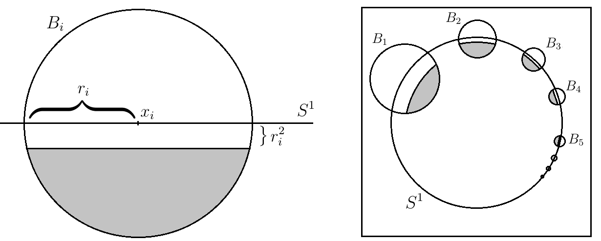
Refer to caption
Figure 1. Construction of a doubling measure which is not doubling after restricting to the unit ball

We observe that 2-dimensional Lebesgue measure μ\mu on XX is doubling, but that the restriction of μ\mu to B⁡(0,1)B(0,1) is not doubling. It is easy to see that there exists a uniform constant c>0c>0 such that for x∈Xx\in X and r∈(0,1)r\in(0,1) we have c​r2⩽μ⁡(B⁡(x,r))⩽π​r2cr^{2}\leqslant\mu(B(x,r))\leqslant\pi r^{2}. It follows that μ\mu is doubling (with upper regularity dimension 2). We now consider the restricted measure ν=μ|B⁡(0,1)\nu=\mu|_{B(0,1)} and compare the masses of B⁡(xi,ri)B(x_{i},r_{i}) and B⁡(xi,2​ri)B(x_{i},2r_{i}). For large enough ii we have ν⁡(B⁡(xi,2​ri))⩾(π​(2​ri)2−π​ri2)/3=π​ri2\nu(B(x_{i},2r_{i}))\geqslant(\pi(2r_{i})^{2}-\pi r_{i}^{2})/3=\pi r_{i}^{2} and ν⁡(B⁡(xi,ri))⩽4​ri3\nu(B(x_{i},r_{i}))\leqslant 4r_{i}^{3}. Therefore

ν⁡(B⁡(xi,2​ri))ν⁡(B⁡(xi,ri))⩾π​ri24​ri3=π4​ri→∞\frac{\nu(B(x_{i},2r_{i}))}{\nu(B(x_{i},r_{i}))}\geqslant\frac{\pi r_{i}^{2}}{4r_{i}^{3}}=\frac{\pi}{4r_{i}}\to\infty

and so ν\nu is not doubling.

2.2. Self-similar measures

In this section we compute the upper regularity dimension of self-similar measures satisfying the strong separation condition. We emphasise that this separation assumption is natural because self-similar measures not satisfying the strong separation condition are typically not doubling and so have upper regularity dimension equal to +∞+\infty.

Let ℐ\mathcal{I} be a finite index set and {Si}i∈ℐ\left\{S_{i}\right\}_{i\in\mathcal{I}} be a finite collection of contraction maps on a compact subset of ℝd\mathbb{R}^{d}. Such a collection is known as an iterated function system (IFS). Also let {pi}i∈ℐ\{p_{i}\}_{i\in\mathcal{I}} be a collection of probabilities associated with the maps {Si}i∈ℐ\{S_{i}\}_{i\in\mathcal{I}}, i.e. we assume that for each i∈ℐi\in\mathcal{I} we have pi>0p_{i}>0 and ∑i∈ℐpi=1\sum_{i\in\mathcal{I}}p_{i}=1. There is a unique non-empty compact set FF satisfying

F=⋃i∈ℐSi​(F)F=\displaystyle\bigcup_{i\in\mathcal{I}}S_{i}(F)

and a unique Borel probability measure μ\mu satisfying

μ=∑i∈ℐpi​μ∘Si−1\mu=\sum_{i\in\mathcal{I}}p_{i}\mu\circ S_{i}^{-1}

which is fully supported on FF, see [F, Chapter 9] and the references therein. When all of the contractions SiS_{i} are similarities, with similarity ratio ci∈(0,1)c_{i}\in\left(0,1\right), then FF is called a self-similar set and μ\mu is called a self-similar measure. We refer the reader to [F] for a more in depth discussion of IFSs and self-similar sets and measures.

Refer to caption
Refer to caption
Refer to caption
Figure 2. A self-similar Sierpiński triangle and two perspectives of a self-similar Sierpiński tetrahedron.

We say that the IFS (and associated set FF and measure μ\mu) satisfy the strong separation condition (SSC) if Si​(F)∩Sj​(F)=∅S_{i}(F)\cap S_{j}(F)=\emptyset for all distinct i,j∈ℐi,j\in\mathcal{I}. This is a natural assumption in the context of the upper regularity dimension. For example, if the defining IFS consists of the maps x↦x/2x\mapsto x/2 and x↦x/2+1/2x\mapsto x/2+1/2, then the SSC is not satisfied and one easily verifies that μ\mu is doubling if and only if both probabilities are equal to 1/2 and in this case μ\mu is Ahlfors-David 1-regular (it is Lebesgue measure on the unit interval).

Theorem 2.4.

Let μ\mu be a self-similar measure as defined above and assume μ\mu satisfies the SSC. Then

dim¯reg​μ=supxdim¯loc​(x,μ)=T⁡(μ)=maxi∈ℐ⁡log⁡pilog⁡ci.\overline{\dim}_{\textup{reg}}\mu=\sup_{x}\overline{\dim}_{\textup{loc}}(x,\mu)=T(\mu)=\max_{i\in\mathcal{I}}\frac{\log p_{i}}{\log c_{i}}.

The Assouad dimension of the self-similar set which supports μ\mu is generally strictly smaller than the upper regularity dimension of μ\mu in this setting. In fact the only case where the Assouad dimension and upper regularity dimensions coincide is when pi=cisp_{i}=c_{i}^{s} where ss is the unique solution of ∑i∈ℐcis=1\sum_{i\in\mathcal{I}}c_{i}^{s}=1. In this case μ\mu is Ahlfors-David ss-regular and all of the notions of dimension for FF and μ\mu coincide and equal ss.

2.3. Self-affine measures

In this section we consider an important class of self-affine measures. Self-affine measures are defined in a similar way to the self-similar measures considered in the previous section, the only difference being that the defining contractions are assumed to be affinities rather than similarities. In general, such measures are much more difficult to handle due to the fact that different rates of distortion can occur in different directions. The specific class of self-affine measures we consider are those supported on Bedford-McMullen carpets, see [B, Mc], and on the higher dimensional analogues, the Bedford-McMullen sponges, see [KP, Ol2]. These sets (and measures) came to prominence recently when they were used by Das and Simmons to provide a counter example to an important and long-standing conjecture in dynamical systems [DS]. In particular, there exists a surprising example of a sponge in ℝ3\mathbb{R}^{3} whose Hausdorff dimension cannot be approximated by the Hausdorff dimension of measures invariant under the natural associated dynamical system. We assume the measures satisfy the very strong separation condition, which was used by Olsen in [Ol2]. Again, this is the natural condition to assume in the context of upper regularity dimension because without this assumption the self-affine measures tend not to be doubling, see [LWW, FH].

Let d⩾2d\geqslant 2 be an integer and fix integers 1<n1<n2⋯<nd1<n_{1}<n_{2}\cdots<n_{d}. Choose a subset ℐ\mathcal{I} of ∏l=1d{0,…,nl−1}\prod_{l=1}^{d}\left\{0,\ldots,n_{l}-1\right\} and for i=(i1,…,id)∈ℐ\textbf{i}=(i_{1},\ldots,i_{d})\in\mathcal{I} let Si:[0,1]d→[0,1]dS_{\textbf{i}}\colon[0,1]^{d}\rightarrow[0,1]^{d} be defined by

Si​(x1,x2​…,xd)=(x1+i1n1,x2+i2n2,…,xd+idnd).S_{\textbf{i}}(x_{1},x_{2}\ldots,x_{d})=\left(\frac{x_{1}+i_{1}}{n_{1}},\frac{x_{2}+i_{2}}{n_{2}},\ldots,\frac{x_{d}+i_{d}}{n_{d}}\right).

Finally, consider the IFS {Si}i∈ℐ\{S_{i}\}_{i\in\mathcal{I}} acting on [0,1]d[0,1]^{d} and let {pi}i∈ℐ\{p_{i}\}_{i\in\mathcal{I}} be an associated probability vector as before. Let FF be the associated attractor of this IFS, which is a self-affine set since each of the defining contractions is an affinity, and let μ\mu be the associated self-affine measure. We can now state the separation condition we require, which we note is strictly stronger than the SSC.

Refer to caption
Refer to caption
Refer to caption
Figure 3. Three perspectives of the self-affine sponge defined by the data: d=3d=3, n1=3n_{1}=3, n2=4n_{2}=4, n3=5n_{3}=5 and ℐ={(0,0,0),(0,2,0),(2,1,1)\mathcal{I}=\{(0,0,0),(0,2,0),(2,1,1), (2,3,4)(2,3,4), (0,0,4)}(0,0,4)\}. The origin is marked by a red dot to indicate orientation.
Definition 2.5 (VSSC, [Ol2]).

A self-affine sponge FF (associated to an index set ℐ\mathcal{I}) satisfies the very strong separation condition (VSSC) if the following condition holds. If l=1,…,dl=1,\ldots,d and (i1,…,id)(i_{1},\ldots,i_{d}), (j1,…,jd)∈ℐ(j_{1},\ldots,j_{d})\in\mathcal{I} satisfy i1=j1,…,il−1=jl−1i_{1}=j_{1},\ldots,i_{l-1}=j_{l-1} and il≠jli_{l}\neq j_{l}, then |il−jl|>1\lvert i_{l}-j_{l}\rvert>1.

Before we state our result, we need to introduce some more notation. For l=1,…,dl=1,\dots,d and i=(i1,…,id)∈ℐ\textbf{i}=(i_{1},\ldots,i_{d})\in\mathcal{I} let

pl​(𝐢)=p⁡(il|i1,…,il−1)=∑j=(j1,…,jd)∈ℐj1=i1,…,jl−1=il−1,jl=ilpj∑j=(j1,…,jd)∈ℐj1=i1,…,jl−1=il−1pjp_{l}(\mathbf{i})=p(i_{l}|i_{1},\ldots,i_{l-1})=\frac{\displaystyle\sum_{\begin{subarray}{c}\textbf{j}=\left(j_{1},\ldots,j_{d}\right)\in\mathcal{I}\\ j_{1}=i_{1},\ldots,j_{l-1}=i_{l-1},j_{l}=i_{l}\end{subarray}}p_{\textbf{j}}}{\displaystyle\sum_{\begin{subarray}{c}\textbf{j}=\left(j_{1},\ldots,j_{d}\right)\in\mathcal{I}\\ j_{1}=i_{1},\ldots,j_{l-1}=i_{l-1}\end{subarray}}p_{\textbf{j}}}

if (i1,…,il,il+1,…,id)∈ℐ(i_{1},\ldots,i_{l},i_{l+1},\ldots,i_{d})\in\mathcal{I} for some il+1,…,idi_{l+1},\ldots,i_{d} and 00 otherwise. These numbers have a clear interpretation: pl​(𝐢)p_{l}(\mathbf{i}) is the conditional probability that the llth digit of an element of ℐ\mathcal{I} coincides with the llth digit of 𝐢\mathbf{i}, given that the first l−1l-1 coordinates did. Note that when l=1l=1 we are conditioning on the entire space and so the denominator of the above conditional probability is taken to be 1.

Theorem 2.6.

Let μ\mu be a self-affine measure on a Bedford-McMullen sponge satisfying the VSSC. Then

dim¯reg​μ=∑l=1dmax𝐢∈ℐ⁡−log⁡pl​(𝐢)log⁡nl.\overline{\dim}_{\textup{reg}}\mu=\sum_{l=1}^{d}\max_{\mathbf{i}\in\mathcal{I}}\frac{-\log p_{l}(\mathbf{i})}{\log n_{l}}.

Formulae for supxdim¯loc​(x,μ)\sup_{x}\overline{\dim}_{\text{loc}}(x,\mu) and T⁡(μ)T(\mu) for the self-affine measures μ\mu we consider in this section can be found in [Ol2], where the notation a¯\overline{a} and A¯\overline{A} was used, respectively. Also, the Assouad dimension of these sponges was first computed by Mackay [M] in the case d=2d=2 and in [FH] for general dd.

We will now discuss a family of examples designed to demonstrate that all of the notions of dimension we discuss here can be distinct for self-affine measures. In particular, the upper regularity dimension can be strictly greater than the Assouad dimension, supremum of the upper local dimensions and the ‘top of the spectrum’, T⁡(μ)T(\mu). This behaviour was not seen in the self-similar case.

Let d=2d=2, n1=3n_{1}=3, n2=4n_{2}=4, ℐ={(0,2),(2,1),(2,3)}\mathcal{I}=\left\{(0,2),(2,1),(2,3)\right\} and p(0,2)=ε,p(2,1)=1−3​ε/2p_{(0,2)}=\varepsilon,\,p_{(2,1)}=1-3\varepsilon/2 and p(2,3)=ε/2p_{(2,3)}=\varepsilon/2 where we allow ε\varepsilon to vary in the interval (0,1/2](0,1/2]. We write FF for the self-affine carpet and μ\mu for the self-affine measure associated with this data. Observe that the VSSC is satisfied and so our results apply. Theorem 2.6 yields

dim¯reg​μ=−log⁡εlog⁡3+−log⁡ε/21−εlog⁡4,\overline{\dim}_{\textup{reg}}\mu=\frac{-\log\varepsilon}{\log 3}+\frac{-\log\frac{\varepsilon/2}{1-\varepsilon}}{\log 4},

Mackay’s result [M] gives

dimAF=log⁡2log⁡3+log⁡2log⁡4,\dim_{\text{A}}F=\frac{\log 2}{\log 3}+\frac{\log 2}{\log 4},

and, using results from [Ol2],

supx∈Fdim¯loc​(x,μ)=max⁡{−log⁡εlog⁡3,−log⁡(1−ε)log⁡3+−log⁡ε/21−εlog⁡4},\sup_{x\in F}\overline{\dim}_{\text{loc}}(x,\mu)=\max\left\{\frac{-\log\varepsilon}{\log 3},\frac{-\log(1-\varepsilon)}{\log 3}+\frac{-\log\frac{\varepsilon/2}{1-\varepsilon}}{\log 4}\right\},

(which has a phase transition at ε≈0.066\varepsilon\approx 0.066), and

T⁡(μ)=−log⁡εlog⁡3+log⁡2log⁡4.T(\mu)=\frac{-\log\varepsilon}{\log 3}+\frac{\log 2}{\log 4}.

For ε∈(0,1/2)\varepsilon\in(0,1/2) these quantities are all distinct and for ε=1/2\varepsilon=1/2 the measure is the ‘coordinate uniform measure’ from [FH] which has upper regularity dimension precisely equal to the Assouad dimension.

ε\varepsilon1−3​ε21-\frac{3\varepsilon}{2}ε2\frac{\varepsilon}{2}
000.10.10.20.20.30.30.40.40.50.50022446688ε\varepsilondim¯reg​μ\overline{\dim}_{\textup{reg}}\muT⁡(μ)T(\mu)supxdim¯loc​(x,μ)\sup_{x}\overline{\dim}_{\text{loc}}(x,\mu)dimAF\dim_{\text{A}}F
Figure 4. Left: the affine maps and associated probabilities. Right: a plot showing the four different ‘dimensions’ as ε\varepsilon varies.

2.4. Measures on sequences

When one first meets the Assouad dimension, the first interesting example is often that the set {1/n}n∈ℕ\left\{1/n\right\}_{n\in\mathbb{N}} has Assouad dimension 1, which is strictly larger than the upper and lower box dimensions which are both 1/2. Since this example is so prevalent, we decided to investigate the upper regularity dimensions of natural families of measures supported on such sets. For simplicity we restrict our examples to countable subsets of [0,1][0,1] with one accumulation point at 0 and measures equal to the sum of decaying point masses on the elements of the set. The interplay between the rate of convergence of the points in the set and the rate of decay of the point masses will turn out to be paramount to understanding the dimension of the measure, and to emphasise this we provide exact results for some simple cases where the rates of convergence are either polynomial or exponential. However, it could be interesting in the future to study sequences with other decay rates, for example stretched exponential decay anba^{n^{b}} for a,b∈(0,1)a,b\in(0,1), n∈ℕn\in\mathbb{N}.

More concretely, consider the set {xn:n∈ℕ}\left\{x_{n}\ :\ n\in\mathbb{N}\right\} where xn↘0x_{n}\searrow 0 and the sequence of weights {p⁡(n):n∈ℕ}\left\{p(n)\ :\ n\in\mathbb{N}\right\} where p⁡(n)↘0p(n)\searrow 0, and ∑n=1∞p⁡(n)<∞\sum_{n=1}^{\infty}p(n)<\infty. The measure we are interested in is

μ=1∑n=1∞p⁡(n)​∑n=1∞p⁡(n)​δxn\mu=\frac{1}{\sum_{n=1}^{\infty}p(n)}\sum_{n=1}^{\infty}p(n)\delta_{x_{n}}

where δxn\delta_{x_{n}} is a point mass at xnx_{n}.

Theorem 2.7.

Let μ\mu be as above.

  1. (1)

    Polynomial-polynomial: Let λ>0\lambda>0 and ω>1\omega>1 and suppose xn=n−λx_{n}=n^{-\lambda} and p⁡(n)=n−ωp(n)=n^{-\omega}. Then

    dim¯reg​μ=max⁡{1,ω−1λ}=max⁡{dimAsupp​(μ),supxdim¯loc​(x,μ)}.\overline{\dim}_{\textup{reg}}\mu\ =\ \max\left\{1,\,\frac{\omega-1}{\lambda}\right\}\ =\ \max\left\{\dim_{\textup{A}}\textup{supp}(\mu),\,\sup_{x}\overline{\dim}_{\textup{loc}}(x,\mu)\right\}.
  2. (2)

    Exponential-exponential: Let λ,ω∈(0,1)\lambda,\omega\in(0,1) and suppose xn=λnx_{n}=\lambda^{n} and p⁡(n)=ωnp(n)=\omega^{n}. Then

    dim¯reg​μ=log⁡ωlog⁡λ=supxdim¯loc​(x,μ)> 0=dimAsupp​(μ).\overline{\dim}_{\textup{reg}}\mu\ =\ \frac{\log\omega}{\log\lambda}\ =\ \sup_{x}\overline{\dim}_{\textup{loc}}(x,\mu)\ >\ 0\ =\ \dim_{\textup{A}}\textup{supp}(\mu).
  3. (3)

    Mixed rates: If

    1. (i)

      xn=n−λx_{n}=n^{-\lambda} (λ>0)(\lambda>0) and p⁡(n)=ωnp(n)=\omega^{n} (0<ω<1)(0<\omega<1); or

    2. (ii)

      xn=λnx_{n}=\lambda^{n} (0<λ<1)(0<\lambda<1) and p⁡(n)=n−ωp(n)=n^{-\omega} (ω>1)(\omega>1),

    then μ\mu is not doubling, and so dim¯reg​μ=∞\overline{\dim}_{\textup{reg}}\mu=\infty.

The above theorem can be summarised by the following table, for suitable values of ω\omega and λ\lambda:

p⁡(n)∖xnp(n)\setminus x_{n} n−λn^{-\lambda} λn\lambda^{n}
n−ωn^{-\omega} max⁡{1,ω−1λ}\max\left\{1,\frac{\omega-1}{\lambda}\right\} ∞\infty
ωn\omega^{n} ∞\infty log⁡ωlog⁡λ\frac{\log\omega}{\log\lambda}

3. Proofs

We prove Theorem 2.1 in Section 3.2 followed by Theorem 2.2 on weak tangents in Section 3.3. Section 3.4 will concern self-similar measures and will include a proof of Theorem 2.4. Self-affine measures and the proof of Theorem 2.6 will be dealt with in Section 3.5 along with some additional notation needed to study Bedford-McMullen sponges. Finally, Theorem 2.7 will be proved in Section 3.6. Any notation introduced in a subsection should only be used in that proof, but any notation used in the first two sections is assumed throughout.

3.1. Proof of equivalence of doubling and finite upper regularity dimension

As we mentioned in the introduction, a measure is doubling if and only if it has finite upper regularity dimension. Here we state a quantifiable version of this fundamental fact and include our own short proof for completeness. Given θ∈(0,1)\theta\in(0,1) let

C(θ)=sup{μ⁡(B⁡(x,R))μ⁡(B⁡(x,θ​R)):x∈supp(μ),R>0}⩾1C(\theta)=\sup\left\{\frac{\mu(B(x,R))}{\mu(B(x,\theta R))}\ :\ x\in\text{supp}(\mu),R>0\right\}\geqslant 1

and note that C⁡(1/2)C(1/2) is the ‘doubling constant’ from the definition of doubling. Also recall that if C⁡(θ)<∞C(\theta)<\infty for some θ∈(0,1)\theta\in(0,1), then C⁡(θ)<∞C(\theta)<\infty for all θ∈(0,1)\theta\in(0,1).

Proposition 3.1.

A locally finite Borel measure is doubling if and only if dim¯reg​μ<∞\overline{\dim}_{\textup{reg}}\mu<\infty. Moreover, we have

dim¯reg​μ⩽infθ∈(0,1)log⁡C⁡(θ)−log⁡θ.\overline{\dim}_{\textup{reg}}\mu\leqslant\inf_{\theta\in(0,1)}\frac{\log C(\theta)}{-\log\theta}.
Proof.

If dim¯reg​μ<∞\overline{\dim}_{\textup{reg}}\mu<\infty then it follows immediately from the definition that μ\mu is doubling. For the reverse implication, assume that μ\mu is doubling and let θ∈(0,1)\theta\in(0,1). Therefore, for all x∈supp​(μ)x\in\text{supp}(\mu) and R>0R>0

μ⁡(B⁡(x,R))μ⁡(B⁡(x,θ​R))⩽C⁡(θ).\frac{\mu(B(x,R))}{\mu(B(x,\theta R))}\leqslant C(\theta).

Fix 0<r<R0<r<R and define kk to be the unique integer such that R​θk>r⩾R​θk+1R\theta^{k}>r\geqslant R\theta^{k+1}. Then by telescoping we obtain

μ⁡(B⁡(x,R))μ⁡(B⁡(x,r))=μ⁡(B⁡(x,R))μ⁡(B⁡(x,θ​R))×μ⁡(B⁡(x,θ​R))μ⁡(B⁡(x,θ2​R))×⋯×μ⁡(B⁡(x,θk​R))μ⁡(B⁡(x,θk+1​R))×μ⁡(B⁡(x,θk+1​R))μ⁡(B⁡(x,r)).\frac{\mu(B(x,R))}{\mu(B(x,r))}=\frac{\mu(B(x,R))}{\mu(B(x,\theta R))}\times\frac{\mu(B(x,\theta R))}{\mu(B(x,\theta^{2}R))}\times\cdots\times\frac{\mu(B(x,\theta^{k}R))}{\mu(B(x,\theta^{k+1}R))}\times\frac{\mu(B(x,\theta^{k+1}R))}{\mu(B(x,r))}.

Thus

μ⁡(B⁡(x,R))μ⁡(B⁡(x,r))⩽C(θ)k+1μ⁡(B⁡(x,θk+1​R))μ⁡(B⁡(x,r))⩽C(θ)log⁡(r/R)/log⁡θ+1=C(θ)(Rr)−logC(θ)/logθ\frac{\mu(B(x,R))}{\mu(B(x,r))}\leqslant C(\theta)^{k+1}\frac{\mu(B(x,\theta^{k+1}R))}{\mu(B(x,r))}\leqslant C(\theta)^{\log(r/R)/\log\theta+1}=C(\theta)\left(\frac{R}{r}\right)^{-\log C(\theta)/\log\theta}

and hence dim¯regμ⩽−logC(θ)/logθ<∞\overline{\dim}_{\textup{reg}}\mu\leqslant-\log C(\theta)/\log\theta<\infty, as required. ∎

3.2. Proof of Theorem 2.1: general relationships

Let μ\mu be a Borel probability measure supported on a compact set X⊆ℝdX\subseteq\mathbb{R}^{d}. Let 0<s<T⁡(μ)0<s<T(\mu), dim¯reg​μ<t<∞\overline{\dim}_{\textup{reg}}\mu<t<\infty and q<0q<0. By definition there exists a constant C⩾1C\geqslant 1 such that for all x∈Xx\in X and for all 0<r<10<r<1

μ⁡(B⁡(x,1))μ⁡(B⁡(x,r))⩽C​(1r)t.\frac{\mu(B(x,1))}{\mu(B(x,r))}\leqslant C\left(\frac{1}{r}\right)^{t}.

In particular, this guarantees

μ​(B⁡(x,r))q⩽1Cq​μ​(B⁡(x,1))q​rq​t\mu(B(x,r))^{q}\leqslant\frac{1}{C^{q}}\mu(B(x,1))^{q}r^{qt}

and, moreover,

Mrq​(μ)⩽c​r−d​rq​tM_{r}^{q}(\mu)\leqslant cr^{-d}r^{qt}

where c>0c>0 is a constant independent of rr and where the r−dr^{-d} term comes from an upper bound on rr-packings of X⊆ℝdX\subseteq\mathbb{R}^{d}. Therefore

s​q>τ¯​(q)⩾q​t−dsq>\underline{\tau}(q)\geqslant qt-d

and so s<t−d/qs<t-d/q for any q<0q<0. By letting q→−∞q\rightarrow-\infty this yields s⩽ts\leqslant t, which is sufficient to prove that T⁡(μ)⩽dim¯reg​μT(\mu)\leqslant\overline{\dim}_{\textup{reg}}\mu.

All that remains is to prove that T⁡(μ)⩾dim¯loc​(x,μ)T(\mu)\geqslant\overline{\dim}_{\text{loc}}(x,\mu) for all x∈Xx\in X. As such, let x∈Xx\in X and u>T⁡(μ)u>T(\mu) which implies that τ¯​(q)⩾u​q\underline{\tau}(q)\geqslant uq for some q<0q<0 which we fix. Therefore, given ε>0\varepsilon>0, there exists a constant Cε>0C_{\varepsilon}>0 such that

Mrq​(μ)⩽Cε​ru​q−εM_{r}^{q}(\mu)\leqslant C_{\varepsilon}r^{uq-\varepsilon}

for all r∈(0,1)r\in(0,1). Since {B⁡(x,r)}\{B(x,r)\} is an rr-packing of XX, it follows that

μ​(B⁡(x,r))q⩽Mrq​(μ)⩽Cε​ru​q−ε\mu(B(x,r))^{q}\leqslant M_{r}^{q}(\mu)\leqslant C_{\varepsilon}r^{uq-\varepsilon}

and therefore

μ⁡(B⁡(x,r))⩾Cε1/q​ru−ε/q\mu(B(x,r))\geqslant C_{\varepsilon}^{1/q}r^{u-\varepsilon/q}

for all r∈(0,1)r\in(0,1), which proves that dim¯loc​(x,μ)⩽u−ε/q\overline{\dim}_{\text{loc}}(x,\mu)\leqslant u-\varepsilon/q and since ε>0\varepsilon>0 was arbitrary, this completes the proof.

3.3. Weak tangent measures

Let μ\mu be a locally finite Borel measure on ℝd\mathbb{R}^{d}, {Tk}k∈ℕ\left\{T_{k}\right\}_{k\in\mathbb{N}} a sequence of similarities on ℝd\mathbb{R}^{d} with associated contraction ratios {ck}k∈ℕ\{c_{k}\}_{k\in\mathbb{N}}, {pk}k∈ℕ\left\{p_{k}\right\}_{k\in\mathbb{N}} a sequence of positive renormalising numbers, and μ^\hat{\mu} be a corresponding weak tangent measure of μ\mu, that is a Borel measure on ℝd\mathbb{R}^{d} such that

pk​μ∘Tk−1⇀μ^p_{k}\mu\circ T^{-1}_{k}\rightharpoonup\hat{\mu}

where ⇀\rightharpoonup means weak convergence. The Portmanteau Theorem (see [Ma, Theorem 1.24]) says that this is equivalent to

limk→∞pk​μ∘Tk−1​(A)=μ^​(A)\lim_{k\rightarrow\infty}p_{k}\mu\circ T^{-1}_{k}(A)=\hat{\mu}(A)

for all μ^\hat{\mu}-continuity sets AA. Recall that A⊆ℝdA\subseteq\mathbb{R}^{d} is a μ^\hat{\mu}-continuity set when μ^​(∂A)=0\hat{\mu}(\partial A)=0 with ∂A\partial A being the boundary of AA. It is a simple exercise to show that for a fixed x∈ℝdx\in\mathbb{R}^{d}, all but at most countably many balls B⁡(x,r)B(x,r) are μ^\hat{\mu}-continuity sets of ℝd\mathbb{R}^{d}. We now provide a technical lemma which reduces our calculation of the upper regularity dimension of μ^\hat{\mu} to the study of balls which are μ^\hat{\mu}-continuity sets.

Lemma 3.2.

Let ν\nu be a locally finite Borel measure on ℝd\mathbb{R}^{d}. Suppose there exist constants CC and ss such that for all x∈supp​(ν)x\in\textup{supp}(\nu) and 0<r<R0<r<R such that B⁡(x,R)B(x,R) and B⁡(x,r)B(x,r) are ν\nu-continuity sets, we have

ν⁡(B⁡(x,R))ν⁡(B⁡(x,r))⩽C​(Rr)s.\frac{\nu(B(x,R))}{\nu(B(x,r))}\leqslant C\left(\frac{R}{r}\right)^{s}.

Then dim¯reg​ν⩽s.\overline{\dim}_{\textup{reg}}\nu\leqslant s.

Proof.

Assume

ν⁡(B⁡(x,R))ν⁡(B⁡(x,r))⩽C​(Rr)s\frac{\nu(B(x,R))}{\nu(B(x,r))}\leqslant C\left(\frac{R}{r}\right)^{s}

holds for all ν\nu-continuity balls. Fix x∈supp​(ν)x\in\textup{supp}(\nu) and let 0<r<R0<r<R be arbitrary. Since there are at most countably many problematic radii, there must exist constants θ1​(x,r),θ2​(x,R)∈[1,2]\theta_{1}(x,r),\theta_{2}(x,R)\in[1,2] such that B⁡(x,θ1​(x,r)−1​r)B(x,\theta_{1}(x,r)^{-1}r) and B⁡(x,θ2​(x,R)​R)B(x,\theta_{2}(x,R)R) are ν\nu-continuity balls. Thus

ν⁡(B⁡(x,R))ν⁡(B⁡(x,r))⩽ν⁡(B⁡(x,θ2​(x,R)​R))ν⁡(B⁡(x,θ1​(x,r)−1​r))⩽C​(θ2​(x,R)​Rθ1​(x,r)−1​r)s⩽4s​C​(Rr)s\frac{\nu(B(x,R))}{\nu(B(x,r))}\leqslant\frac{\nu(B(x,\theta_{2}(x,R)R))}{\nu(B(x,\theta_{1}(x,r)^{-1}r))}\leqslant C\left(\frac{\theta_{2}(x,R)R}{\theta_{1}(x,r)^{-1}r}\right)^{s}\leqslant 4^{s}C\left(\frac{R}{r}\right)^{s}

and it follows that dim¯reg​ν⩽s.\overline{\dim}_{\textup{reg}}\nu\leqslant s. ∎

We now return to proving Theorem 2.2. Let x∈supp​(μ^)x\in\textup{supp}(\hat{\mu}) and ρ>0\rho>0 be such that B⁡(x,ρ)B(x,\rho) is a μ^\hat{\mu}-continuity set. Therefore

limk→∞pk​μ∘Tk−1​(B⁡(x,ρ))=μ^​(B⁡(x,ρ)).\lim_{k\rightarrow\infty}p_{k}\mu\circ T^{-1}_{k}(B(x,\rho))=\hat{\mu}(B(x,\rho)).

Therefore, for sufficiently large kk,

(3.1) 12​pk​μ∘Tk−1​(B⁡(x,ρ))⩽μ^​(B⁡(x,ρ))⩽2​pk​μ∘Tk−1​(B⁡(x,ρ)).\frac{1}{2}p_{k}\mu\circ T^{-1}_{k}(B(x,\rho))\leqslant\hat{\mu}(B(x,\rho))\leqslant 2p_{k}\mu\circ T^{-1}_{k}(B(x,\rho)).

Let ε>0\varepsilon>0 and 0<r<R0<r<R be such that both B⁡(x,R)B(x,R) and B⁡(x,r)B(x,r) are μ^\hat{\mu}-continuity sets and choose kk large enough so that (3.1) holds for ρ=r\rho=r and ρ=R\rho=R. In particular,

μ^​(B​(x,R))μ^​(B​(x,r))⩽4​pk​μ∘Tk−1​(B⁡(x,R))pk​μ∘Tk−1​(B⁡(x,r))=4​μ⁡(Tk−1​(B⁡(x,R)))μ⁡(Tk−1​(B⁡(x,r))).\frac{\hat{\mu}(B(x,R))}{\hat{\mu}(B(x,r))}\leqslant 4\frac{p_{k}\mu\circ T^{-1}_{k}(B(x,R))}{p_{k}\mu\circ T^{-1}_{k}(B(x,r))}=4\frac{\mu(T^{-1}_{k}(B(x,R)))}{\mu(T^{-1}_{k}(B(x,r)))}.

Note that TkT_{k} is a similarity of contraction ratio ck>0c_{k}>0 and so Tk−1​(B⁡(x,R))=B⁡(Tk−1​(x),ck−1​R)T_{k}^{-1}(B(x,R))=B(T_{k}^{-1}(x),c_{k}^{-1}R). Thus

μ^​(B​(x,R))μ^​(B​(x,r))\displaystyle\frac{\hat{\mu}(B(x,R))}{\hat{\mu}(B(x,r))} ⩽4​μ⁡(B⁡(Tk−1​(x),ck−1​R))μ⁡(B⁡(Tk−1​(x),ck−1​r)).\displaystyle\leqslant 4\frac{\mu(B(T_{k}^{-1}(x),c_{k}^{-1}R))}{\mu(B(T_{k}^{-1}(x),c_{k}^{-1}r))}.

Here we wish to apply the definition of the upper regularity dimension of μ\mu, but we cannot do this directly since Tk−1​(x)T_{k}^{-1}(x) does not have to be in supp​(μ)\text{supp}(\mu). However, we can assume kk is large enough (depending on rr) so that there exists x′x^{\prime} in the support of μ∘Tk−1\mu\circ T_{k}^{-1} which is at distance at most r/2r/2 from xx. Therefore

B⁡(Tk−1​(x′),ck−1​r/2)⊂B⁡(Tk−1​(x),ck−1​r) and B⁡(Tk−1​(x),ck−1​R)⊂B⁡(Tk−1​(x′),2​ck−1​R)B(T_{k}^{-1}(x^{\prime}),c_{k}^{-1}r/2)\subset B(T_{k}^{-1}(x),c_{k}^{-1}r)\qquad\text{ and }\qquad B(T_{k}^{-1}(x),c_{k}^{-1}R)\subset B(T_{k}^{-1}(x^{\prime}),2c_{k}^{-1}R)

and Tk−1​(x′)T_{k}^{-1}(x^{\prime}) is in the support of μ\mu. Therefore

μ^​(B​(x,R))μ^​(B​(x,r))\displaystyle\frac{\hat{\mu}(B(x,R))}{\hat{\mu}(B(x,r))} ⩽4​μ⁡(B⁡(Tk−1​(x),ck−1​R))μ⁡(B⁡(Tk−1​(x),ck−1​r))⩽4​μ⁡(B⁡(Tk−1​(x′),2​ck−1​R))μ⁡(B⁡(Tk−1​(x′),ck−1​r/2))\displaystyle\leqslant 4\frac{\mu(B(T_{k}^{-1}(x),c_{k}^{-1}R))}{\mu(B(T_{k}^{-1}(x),c_{k}^{-1}r))}\leqslant 4\frac{\mu(B(T_{k}^{-1}(x^{\prime}),2c_{k}^{-1}R))}{\mu(B(T_{k}^{-1}(x^{\prime}),c_{k}^{-1}r/2))}
⩽4​C​(4​ck−1​Rck−1​r)dim¯reg​μ+ε=41+dim¯reg​μ+ε​C​(Rr)dim¯reg​μ+ε\displaystyle\leqslant 4C\left(\frac{4c_{k}^{-1}R}{c_{k}^{-1}r}\right)^{\overline{\dim}_{\textup{reg}}\mu+\varepsilon}=4^{1+\overline{\dim}_{\textup{reg}}\mu+\varepsilon}C\left(\frac{R}{r}\right)^{\overline{\dim}_{\textup{reg}}\mu+\varepsilon}

where C=C⁡(ε)>0C=C(\varepsilon)>0 is a uniform constant independent of xx, rr and RR which comes from the definition of the upper regularity dimension of μ\mu. Letting ε→0\varepsilon\to 0 proves dim¯reg​μ^⩽dim¯reg​μ\overline{\dim}_{\textup{reg}}\hat{\mu}\leqslant\overline{\dim}_{\textup{reg}}\mu as desired.

3.4. Proof of Theorem 2.4: self-similar measures

There is a natural correspondence between the geometric fractal FF and the symbolic space ℐℕ\mathcal{I}^{\mathbb{N}} (the set of all infinite words over ℐ\mathcal{I}) via the coding map π:ℐℕ→ℝd\pi\colon\mathcal{I}^{\mathbb{N}}\rightarrow\mathbb{R}^{d} defined by

{π⁡(i0,i1,…)}=⋂n=0∞Si0,…,in​(F)\{\pi(i_{0},i_{1},\ldots)\}=\bigcap_{n=0}^{\infty}S_{i_{0},\ldots,i_{n}}(F)

where Si0,…,in=Si0∘⋯∘SinS_{i_{0},\ldots,i_{n}}=S_{i_{0}}\circ\cdots\circ S_{i_{n}}. For i0,i1,…,in−1∈ℐi_{0},i_{1},\ldots,i_{n-1}\in\mathcal{I} we define a cylinder [i0,i1,…,in−1]⊆ℐℕ[i_{0},i_{1},\ldots,i_{n-1}]\subseteq\mathcal{I}^{\mathbb{N}}, to be the set of all words in ℐℕ\mathcal{I}^{\mathbb{N}} whose first nn letters are i0,i1,…,in−1i_{0},i_{1},\ldots,i_{n-1}. The collection of all level nn cylinders corresponds to the nnth level pre-fractal of the attractor. It is well-known that F=π⁡(ℐℕ)F=\pi(\mathcal{I}^{\mathbb{N}}) and the SSC also guarantees that π\pi is a bijection so we may interchange the symbolic and geometric spaces. Also note that ci0⋯cinc_{i_{0}}\cdots c_{i_{n}} is the contraction ratio of the similarity Si0,…,inS_{i_{0},\ldots,i_{n}}, π⁡([i0,i1,…,in])=Si0,…,in​(F)\pi([i_{0},i_{1},\ldots,i_{n}])=S_{i_{0},\ldots,i_{n}}(F) and the μ\mu measure of Si0,…,in​(F)S_{i_{0},\ldots,i_{n}}(F) is pi0⋯pinp_{i_{0}}\cdots p_{i_{n}}. By rescaling if necessary, we may assume without loss of generality that diam(F)=1(F)=1.

We define δ\delta to be the minimal distance between distinct sets Si​(F)S_{i}(F) and Sj​(F)S_{j}(F), that is

δ=min⁡infx∈Si​(F)y∈Sj​(F)i≠j⁡|x−y|.\delta=\min_{i\neq j}\inf_{\begin{subarray}{c}x\in S_{i}(F)\\ y\in S_{j}(F)\end{subarray}}\lvert x-y\rvert.

The SSC guarantees that δ>0\delta>0. Thus the minimal distance between Si0,…,in−1,i​(F)S_{i_{0},\ldots,i_{n-1},i}(F) and Si0,…,in−1,j​(F)S_{i_{0},\ldots,i_{n-1},j}(F) is at least ci0⋯cin−1δc_{i_{0}}\cdots c_{i_{n-1}}\delta for any i0,i1,…,in−1∈ℐi_{0},i_{1},\ldots,i_{n-1}\in\mathcal{I} and i≠ji\neq j.

For x∈Fx\in F with π⁡(i0,i1,…)=x\pi(i_{0},i_{1},\dots)=x for a unique (i0,i1,…)∈ℐℕ(i_{0},i_{1},\dots)\in\mathcal{I}^{\mathbb{N}} and small r>0r>0, we define the integer n⁡(x,r)n(x,r) to be the largest integer such that r⩽ci0ci1⋯cin⁡(x,r)r\leqslant c_{i_{0}}c_{i_{1}}\cdots c_{i_{n(x,r)}} and so

ci0ci1⋯cin⁡(x,r)+1<r⩽ci0ci1⋯cin⁡(x,r).c_{i_{0}}c_{i_{1}}\cdots c_{i_{n(x,r)}+1}<r\leqslant c_{i_{0}}c_{i_{1}}\cdots c_{i_{n(x,r)}}.

We also let m⁡(x,r)m(x,r) be the smallest non-negative integer such that

π⁡([i0,…,im⁡(x,r)])⊂B⁡(x,r/2),\pi([i_{0},\ldots,i_{m(x,r)}])\subset B(x,r/2),

and so, in particular, pi0⋯pim⁡(x,r)⩽μ(B(x,r))p_{i_{0}}\cdots p_{i_{m(x,r)}}\leqslant\mu(B(x,r)). Note that for any x∈Fx\in F, and small r>0r>0, ci0⋯cim⁡(x,r)⩽rc_{i_{0}}\cdots c_{i_{m(x,r)}}\leqslant r. Also π⁡([i0,…,im⁡(x,r)−1])⊄B⁡(x,r/2)\pi([i_{0},\ldots,i_{m(x,r)-1}])\not\subset B(x,r/2) and so ci0⋯cim⁡(x,r)−1⩾r/2c_{i_{0}}\cdots c_{i_{m(x,r)-1}}\geqslant r/2. Using the SSC, we have that for all x=π⁡(i0,…)x=\pi(i_{0},\ldots) and r>0r>0, we have μ(B(x,δ​r2))⩽pi0⋯pin⁡(x,r)\mu(B(x,\frac{\delta r}{2}))\leqslant p_{i_{0}}\cdots p_{i_{n(x,r)}} where δ\delta is the constant determined by the SSC. This is true since B⁡(x,δ​r2)∩F⊆π⁡([i0,…,in⁡(x,r)])B(x,\frac{\delta r}{2})\cap F\subseteq\pi([i_{0},\ldots,i_{n(x,r)}]).

Let x=π⁡(ω)x=\pi(\omega) where ω∈ℐℕ\omega\in\mathcal{I}^{\mathbb{N}} is an infinite string of the symbol ii which maximises log⁡pi/log⁡ci\log p_{i}/\log c_{i}. It follows that n⁡(x,r)>log⁡r/log⁡ci−1n(x,r)>\log r/\log{c_{i}}-1 and therefore

μ⁡(B⁡(x,δ​r/2))⩽pin⁡(x,r)⩽pi−1​rlog⁡pi/log⁡ci\mu(B(x,\delta r/2))\leqslant p_{i}^{n(x,r)}\leqslant p_{i}^{-1}r^{\log p_{i}/\log c_{i}}

and it follows that dim¯loc​(x,μ)⩾log⁡pi/log⁡ci=:t\overline{\dim}_{\text{loc}}(x,\mu)\geqslant\log p_{i}/\log c_{i}=\colon t. Moreover, Theorem 2.1 yields dim¯reg​μ⩾supx∈Fdim¯loc​(x,μ)⩾t\overline{\dim}_{\textup{reg}}\mu\geqslant\sup_{x\in F}\overline{\dim}_{\text{loc}}(x,\mu)\geqslant t. We will now demonstrate the reverse inequality.

As FF satisfies the SSC and μ\mu is a Bernoulli measure, it is doubling (see [Ol1], for example). Thus there exists a constant C⩾1C\geqslant 1 depending only on δ/2<1\delta/2<1 such that μ⁡(B⁡(x,R))μ⁡(B⁡(x,δ​R/2))⩽C\frac{\mu(B(x,R))}{\mu(B(x,\delta R/2))}\leqslant C for any x∈Fx\in F and for any R>0R>0. Let x∈Fx\in F and 0<r<R0<r<R and assume without meaningful loss of generality that n⁡(x,R)<m⁡(x,r)n(x,R)<m(x,r). If this were not true, then R/rR/r is bounded above by a uniform constant – a situation we can safely ignore. Hence

μ⁡(B⁡(x,R))μ⁡(B⁡(x,r))\displaystyle\frac{\mu(B(x,R))}{\mu(B(x,r))} ⩽C​μ⁡(B⁡(x,δ​R/2))μ⁡(B⁡(x,r))\displaystyle\leqslant\ C\frac{\mu(B(x,\delta R/2))}{\mu(B(x,r))}
⩽C​pi0⋯pin⁡(x,R)pi0⋯pim⁡(x,r)\displaystyle\leqslant\ C\frac{p_{i_{0}}\cdots p_{i_{n(x,R)}}}{p_{i_{0}}\cdots p_{i_{m(x,r)}}}
=C1pin⁡(x,R)+1⋯1pim⁡(x,r)\displaystyle=\ C\frac{1}{p_{i_{n(x,R)+1}}}\cdots\frac{1}{p_{i_{m(x,r)}}}
=C(1cin⁡(x,R)+1)log⁡pin⁡(x,R)+1/log⁡cin⁡(x,R)+1⋯(1cim⁡(x,r))log⁡pim⁡(x,r)/log⁡cim⁡(x,r)\displaystyle=\ C\left(\frac{1}{c_{i_{n(x,R)+1}}}\right)^{\log p_{i_{n(x,R)+1}}/\log c_{i_{n(x,R)+1}}}\cdots\left(\frac{1}{c_{i_{m(x,r)}}}\right)^{\log p_{i_{m(x,r)}}/\log c_{i_{m(x,r)}}}
⩽C(1cin⁡(x,R)+1)t⋯(1cim⁡(x,r))t\displaystyle\leqslant\ C\left(\frac{1}{c_{i_{n(x,R)+1}}}\right)^{t}\cdots\left(\frac{1}{c_{i_{m(x,r)}}}\right)^{t}
=C​(1cin⁡(x,R)+1​cim⁡(x,r))t​(ci0ci1⋯cin⁡(x,R)+1ci0ci1⋯cim⁡(x,r)−1)t\displaystyle=\ C\left(\frac{1}{c_{i_{n(x,R)+1}}c_{i_{m(x,r)}}}\right)^{t}\left(\frac{c_{i_{0}}c_{i_{1}}\cdots c_{i_{n(x,R)+1}}}{c_{i_{0}}c_{i_{1}}\cdots c_{i_{m(x,r)-1}}}\right)^{t}
⩽C​(2cmin2)t​(Rr)t\displaystyle\leqslant\ C\left(\frac{2}{c_{\min}^{2}}\right)^{t}\left(\frac{R}{r}\right)^{t}

where cmin=mini∈ℐ⁡cic_{\min}=\min_{i\in\mathcal{I}}c_{i}, is just a constant. The desired upper bound, and Theorem 2.4, follows.

3.5. Proof of Theorem 2.6: self-affine measures

Similar to the previous section, we use the natural correspondence between the self-affine set FF and the symbolic space ℐℕ\mathcal{I}^{\mathbb{N}} (the set of all infinite words over ℐ\mathcal{I}) via the coding map π:ℐℕ→ℝd\pi\colon\mathcal{I}^{\mathbb{N}}\rightarrow\mathbb{R}^{d} defined by

{π⁡(i1,i2,…)}=⋂n=1∞Si1,…,in​(F).\{\pi(\textbf{i}_{1},\textbf{i}_{2},\ldots)\}=\bigcap_{n=1}^{\infty}S_{\textbf{i}_{1},\ldots,\textbf{i}_{n}}(F).

where Si1,…,in=Si1∘⋯∘SinS_{\textbf{i}_{1},\ldots,\textbf{i}_{n}}=S_{\textbf{i}_{1}}\circ\cdots\circ S_{\textbf{i}_{n}}. Recall that elements of ℐ\mathcal{I} have dd coordinates so we write (𝐢1,…)=((i1,1,…,i1,d),…)∈ℐℕ(\mathbf{i}_{1},\ldots)=((i_{1,1},\ldots,i_{1,d}),\ldots)\in\mathcal{I}^{\mathbb{N}}.

Since the cylinders scale by different amounts in different directions, they do not directly approximate a ball in measure. For this reason, we introduce approximate cubes. For r∈(0,1]r\in(0,1], choose the unique integers k1​(r),…,kd​(r)k_{1}(r),\ldots,k_{d}(r), greater than or equal to 0, satisfying

1nlkl​(r)+1<r⩽1nlkl​(r)\frac{1}{n_{l}^{k_{l}(r)+1}}<r\leqslant\frac{1}{n_{l}^{k_{l}(r)}}

for l=1,…,dl=1,\ldots,d. In particular,

−log⁡rlog⁡nl−1<kl​(r)⩽−log⁡rlog⁡nl.\frac{-\log r}{\log n_{l}}-1<k_{l}(r)\leqslant\frac{-\log r}{\log n_{l}}.

Then the approximate cube Q⁡(ω,r)Q(\omega,r) of (approximate) side length rr determined by ω=(i1,i2,…)=((i1,1,…,i1,d),(i2,1,…,i2,d),…)∈ℐℕ\omega=\left(\textbf{i}_{1},\textbf{i}_{2},\ldots\right)=\left((i_{1,1},\dots,i_{1,d}),(i_{2,1},\dots,i_{2,d}),\ldots\right)\in\mathcal{I}^{\mathbb{N}} is defined by

Q(ω,r)={ω′=(j1,j2,…)∈ℐℕ:∀l=1,…,d and ∀t=1,…,kl(r) we have jt,l=it,l}.Q(\omega,r)=\left\{\omega^{\prime}=\left(\textbf{j}_{1},\textbf{j}_{2},\ldots\right)\in\mathcal{I}^{\mathbb{N}}:\forall\,\,l=1,\ldots,d\text{ and }\forall\,\,t=1,\ldots,k_{l}(r)\text{ we have }j_{t,l}=i_{t,l}\right\}.

The geometric analogue is π⁡(Q⁡(ω,r))\pi\left(Q(\omega,r)\right), which is contained in

∏l=1d[i1,lnl+⋯+ikl​(r),lnlkl​(r),i1,lnl+⋯+ikl​(r),lnlkl​(r)+1nlkl​(r)];\prod_{l=1}^{d}\left[\frac{i_{1,l}}{n_{l}}+\cdots+\frac{i_{k_{l}(r),l}}{n_{l}^{k_{l}(r)}}\,,\,\frac{i_{1,l}}{n_{l}}+\cdots+\frac{i_{k_{l}(r),l}}{n_{l}^{k_{l}(r)}}+\frac{1}{n_{l}^{k_{l}(r)}}\right];

a hypercuboid in ℝd\mathbb{R}^{d} aligned with the coordinate axes with side lengths nl−kl​(r)n_{l}^{-k_{l}(r)}, which are all comparable to rr since r⩽nl−kl​(r)<nl​rr\leqslant n_{l}^{-k_{l}(r)}<n_{l}r. Thus the measure of a ball can be closely approximated by the measure of an appropriate approximate cube. This is made precise by the following useful proposition due to Olsen [Ol2, Proposition 6.2.1].

Proposition 3.3 ([Ol2]).

Let ω∈ℐℕ\omega\in\mathcal{I}^{\mathbb{N}} and k∈ℕk\in\mathbb{N}.

  1. (1)

    If the VSSC is satisfied, then B⁡(π⁡(ω),2−1​n1−k)∩F⊆π⁡(Q⁡(ω,n1−k)).B\left(\pi(\omega),2^{-1}n_{1}^{-k}\right)\cap F\subseteq\pi\left(Q\left(\omega,n_{1}^{-k}\right)\right).

  2. (2)

    π⁡(Q⁡(ω,1/n1k))⊆B⁡(π⁡(ω),(n1+⋯+nd)​n1−k).\pi\left(Q\left(\omega,1/n_{1}^{k}\right)\right)\subseteq B\left(\pi(\omega),(n_{1}+\dots+n_{d})n_{1}^{-k}\right).

This proposition means, since we assume the VSSC, that a ball of a particular radius contains, and is contained in, an approximate cube of a comparable radius. Therefore we may replace balls with approximate cubes in the definition of upper regularity dimension, which makes the calculations much easier. For a more in depth explanation of this simplification, see [FH].

Recalling the conditional probabilities p⁡(il|i1,…,il−1)p(i_{l}|i_{1},\ldots,i_{l-1}), defined in Section 2.3, which give the probability of having ili_{l} as the lth\text{l}^{\text{th}} coordinate given the previous ones, we can write down an explicit formula for the μ\mu measure of an approximate cube for any ω∈ℐℕ\omega\in\mathcal{I}^{\mathbb{N}} and r∈(0,1)r\in(0,1):

(3.2) μ⁡(π⁡(Q⁡(ω,r)))=∏l=1d∏j=0kl​(r)−1pl​(σj​ω)\mu(\pi(Q(\omega,r)))=\prod^{d}_{l=1}\prod_{j=0}^{k_{l}(r)-1}p_{l}(\sigma^{j}\omega)

where pl​(ω)=p⁡(i1,l|i1,1,…,i1,l−1)p_{l}(\omega)=p(i_{1,l}|i_{1,1},\ldots,i_{1,l-1}) and σ:ℐℕ→ℐℕ\sigma:\mathcal{I}^{\mathbb{N}}\to\mathcal{I}^{\mathbb{N}} is the left shift. This formula follows immediately from the definition of μ\mu and was first observed by Olsen [Ol2, (6.2)].

For l=1,…,dl=1,\ldots,d, let plmin=minj∈ℐ⁡pl​(𝐣)p_{l}^{\text{min}}=\min_{j\in\mathcal{I}}p_{l}(\mathbf{j}) and let ilmin∈ℐi_{l}^{\min}\in\mathcal{I} be an element achieving this minimum. If such an element is not unique, it does not matter which we choose. Let t=∑l=1d−log⁡plminlog⁡nlt=\sum_{l=1}^{d}\frac{-\log p_{l}^{\text{min}}}{\log n_{l}}, be the target dimension. Let x=π⁡(ω)∈Fx=\pi(\omega)\in F for a (unique) ω∈ℐℕ\omega\in\mathcal{I}^{\mathbb{N}} and 0<r<R⩽10<r<R\leqslant 1. By the above discussion, and Proposition 3.3, we see that

μ⁡(π⁡(Q⁡(ω,Rn1​(n1+⋯+nd))))μ⁡(π⁡(Q⁡(ω,2​n1​r)))⩽μ⁡(B⁡(x,R))μ⁡(B⁡(x,r))⩽μ⁡(π⁡(Q⁡(ω,2​n1​R)))μ⁡(π⁡(Q⁡(ω,rn1​(n1+⋯+nd))))\frac{\mu\left(\pi\left(Q\left(\omega,\frac{R}{n_{1}(n_{1}+\cdots+n_{d})}\right)\right)\right)}{\mu(\pi(Q(\omega,2n_{1}r)))}\ \leqslant\ \frac{\mu(B(x,R))}{\mu(B(x,r))}\ \leqslant\ \frac{\mu(\pi(Q(\omega,2n_{1}R)))}{\mu\left(\pi\left(Q\left(\omega,\frac{r}{n_{1}(n_{1}+\cdots+n_{d})}\right)\right)\right)}

and so to compute dim¯reg​μ\overline{\dim}_{\textup{reg}}\mu it suffices to consider

μ⁡(π⁡(Q⁡(ω,R)))μ⁡(π⁡(Q⁡(ω,r)))\frac{\mu(\pi(Q(\omega,R)))}{\mu(\pi(Q(\omega,r)))}

directly. We begin with an upper bound using (3.2) and for convenience we assume without loss of generality that r<R/ndr<R/n_{d}, which ensures kl​(R)<kl​(r)k_{l}(R)<k_{l}(r) for all ll. We have

μ⁡(π⁡(Q⁡(ω,R)))μ⁡(π⁡(Q⁡(ω,r)))=∏l=1d(∏j=0kl​(R)−1pl​(σj​ω))∏l=1d(∏j=0kl​(r)−1pl​(σj​ω))\displaystyle\frac{\mu(\pi(Q(\omega,R)))}{\mu(\pi(Q(\omega,r)))}\ =\ \frac{\prod_{l=1}^{d}\left(\prod_{j=0}^{k_{l}(R)-1}p_{l}(\sigma^{j}\omega)\right)}{\prod_{l=1}^{d}\left(\prod_{j=0}^{k_{l}(r)-1}p_{l}(\sigma^{j}\omega)\right)} =1∏l=1d(∏j=kl​(R)kl​(r)−1pl​(σj​ω))\displaystyle=\ \frac{1}{\prod_{l=1}^{d}\left(\prod_{j=k_{l}(R)}^{k_{l}(r)-1}p_{l}(\sigma^{j}\omega)\right)}
⩽∏l=1d1∏j=kl​(R)kl​(r)−1plmin\displaystyle\leqslant\ \prod_{l=1}^{d}\frac{1}{\prod_{j=k_{l}(R)}^{k_{l}(r)-1}p_{l}^{\text{min}}}
=∏l=1d(1plmin)kl​(r)−kl​(R)\displaystyle=\ \prod_{l=1}^{d}\left(\frac{1}{p_{l}^{\text{min}}}\right)^{k_{l}(r)-k_{l}(R)}
⩽∏l=1d(1plmin)−logr/lognl+logR/lognl+1\displaystyle\leqslant\ \prod_{l=1}^{d}\left(\frac{1}{p_{l}^{\text{min}}}\right)^{-\log r/\log n_{l}+\log R/\log n_{l}+1}
⩽p−d​(Rr)t\displaystyle\leqslant\ p^{-d}\left(\frac{R}{r}\right)^{t}

where p=minl⁡plmin>0p=\min_{l}p_{l}^{\text{min}}>0 is a constant. It follows that dim¯reg​μ⩽t\overline{\dim}_{\textup{reg}}\mu\leqslant t.

For the lower bound, we have to be a little more careful with the relationship between RR and rr. Again we assume that r<R/ndr<R/n_{d}, which ensures kl​(R)<kl​(r)k_{l}(R)<k_{l}(r) for all ll. However, for technical reasons we also require kl​(R)>kl+1​(r)k_{l}(R)>k_{l+1}(r) for all l=1,…,d−1l=1,\dots,d-1. For this it is sufficient to assume

(nl​R)log⁡nl+1log⁡nl<r(n_{l}R)^{\frac{\log n_{l+1}}{\log n_{l}}}<r

and fortunately we can choose rr satisfying both of these conditions simultaneously. This is where we use the fact that the nln_{l} are strictly increasing. Moreover, we can choose a sequence of pairs (r,R)(r,R) such that R→0R\to 0, R/r→∞R/r\to\infty and

(nl​R)log⁡nl+1log⁡nl<r<R/nd.(n_{l}R)^{\frac{\log n_{l+1}}{\log n_{l}}}<r<R/n_{d}.

Let R,rR,r be a pair from this sequence and observe that

(3.3) kd​(R)<kd​(r)<kd−1​(R)<kd−1​(r)<⋯<k2​(R)<k2​(r)<k1​(R)<k1​(r).k_{d}(R)<k_{d}(r)<k_{d-1}(R)<k_{d-1}(r)<\cdots<k_{2}(R)<k_{2}(r)<k_{1}(R)<k_{1}(r).

Let ω∈ℐℕ\omega\in\mathcal{I}^{\mathbb{N}} be chosen such that

ω\displaystyle\omega =(i1,…,ikd​(R),idmin,…,idmin,ikd​(r)+1,…,ik2​(R)CLOSE,\displaystyle=(i_{1},\ldots,i_{k_{d}(R)},i_{d}^{\text{min}},\ldots,i_{d}^{\text{min}},i_{k_{d}(r)+1},\ldots,i_{k_{2}(R)},
OPENi2min,…,i2min,ik2​(r)+1,…,ik1​(R),i1min,…,i1min,ik1​(r)+1,…).\displaystyle i_{2}^{\text{min}},\ldots,i_{2}^{\text{min}},i_{k_{2}(r)+1},\ldots,i_{k_{1}(R)},i_{1}^{\text{min}},\ldots,i_{1}^{\text{min}},i_{k_{1}(r)+1},\ldots).

where the coordinates not specified as ilmini_{l}^{\text{min}} (for some l∈{1,…,d}l\in\{1,\dots,d\}) are arbitrary. In particular, we insist that the coordinates ikl​(R)+1,…,ikl​(r)i_{k_{l}(R)+1},\dots,i_{k_{l}(r)} are all equal to ilmini_{l}^{\min}. Note that we use (3.3) here. We have

μ⁡(π⁡(Q⁡(ω,R)))μ⁡(π⁡(Q⁡(ω,r)))=∏l=1d(∏j=0kl​(R)−1pl​(σj​ω))∏l=1d(∏j=0kl​(r)−1pl​(σj​ω))\displaystyle\frac{\mu(\pi(Q(\omega,R)))}{\mu(\pi(Q(\omega,r)))}\ =\ \frac{\prod_{l=1}^{d}\left(\prod_{j=0}^{k_{l}(R)-1}p_{l}(\sigma^{j}\omega)\right)}{\prod_{l=1}^{d}\left(\prod_{j=0}^{k_{l}(r)-1}p_{l}(\sigma^{j}\omega)\right)} =1∏l=1d(∏j=kl​(R)kl​(r)−1pl​(σj​ω))\displaystyle=\ \frac{1}{\prod_{l=1}^{d}\left(\prod_{j=k_{l}(R)}^{k_{l}(r)-1}p_{l}(\sigma^{j}\omega)\right)}
=∏l=1d(1plmin)kl​(r)−kl​(R)\displaystyle=\ \prod_{l=1}^{d}\left(\frac{1}{p_{l}^{\text{min}}}\right)^{k_{l}(r)-k_{l}(R)}
⩾∏l=1d(1plmin)−logr/lognl−1+logR/lognl\displaystyle\geqslant\ \prod_{l=1}^{d}\left(\frac{1}{p_{l}^{\text{min}}}\right)^{-\log r/\log n_{l}-1+\log R/\log n_{l}}
⩾pd​(Rr)t\displaystyle\geqslant\ p^{d}\left(\frac{R}{r}\right)^{t}

where p=minl⁡plmin>0p=\min_{l}p_{l}^{\text{min}}>0 is a constant as before. Since we can choose a sequence of parameters x=π⁡(ω)x=\pi(\omega), r<Rr<R satisfying the above with R/r→∞R/r\to\infty, it follows that dim¯reg​μ⩾t\overline{\dim}_{\textup{reg}}\mu\geqslant t, completing the proof.

3.6. Sequences and associated measures

We start by explaining our method and then we specialise to the particular cases of Theorem 2.7 in subsequent subsections. For convenience, we assume that xk↘0x_{k}\searrow 0, xk−xk+1↘0x_{k}-x_{k+1}\searrow 0 (decreasing gaps) and that p⁡(k)p(k) (k∈ℕk\in\mathbb{N}) can be extended to a decreasing L1L^{1} function pp on the whole of [0,∞)[0,\infty). These conditions are obviously satisfied for the examples we consider. Throughout this section we write f⁡(x)=O⁡(g⁡(x))f(x)=O(g(x)) to mean f⁡(x)⩽C​g​(x)f(x)\leqslant Cg(x) for a constant CC independent of xx.

For 0<r<10<r<1 and x∈supp​(μ)x\in\textup{supp}(\mu), let k¯​(x,r),k¯​(x,r)\overline{k}(x,r),\underline{k}(x,r) be the unique integers such that xk¯​(x,r)+1<x−r⩽xk¯​(x,r)x_{\overline{k}(x,r)+1}<x-r\leqslant x_{\overline{k}(x,r)} and xk¯​(x,r)⩽x+r<xk¯​(x,r)−1x_{\underline{k}(x,r)}\leqslant x+r<x_{\underline{k}(x,r)-1} where we adopt the convention that k¯​(x,r)=∞\overline{k}(x,r)=\infty when x−r⩽0x-r\leqslant 0. Therefore

μ⁡(B⁡(x,r))=1∑n=1∞p⁡(n)​∑i=k¯​(x,r)k¯​(x,r)p⁡(i).\mu(B(x,r))=\frac{1}{\sum_{n=1}^{\infty}p(n)}\sum_{i=\underline{k}(x,r)}^{\overline{k}(x,r)}p(i).

Of course there is a possibility that xk¯​(x,r)=xx_{\overline{k}(x,r)}=x when x≠0x\neq 0 and then μ⁡(B⁡(x,r))=μ⁡({x})\mu(B(x,r))=\mu(\left\{x\right\}). Thus, given 0<r<R<10<r<R<1, we will consider three different cases:

  1. (1)

    x∈supp​(μ)∖{0}x\in\textup{supp}(\mu)\setminus\left\{0\right\} such that xk¯​(x,r)=xk¯​(x,R)=xx_{\overline{k}(x,r)}=x_{\overline{k}(x,R)}=x,

  2. (2)

    x∈supp​(μ)∖{0}x\in\textup{supp}(\mu)\setminus\left\{0\right\} such that xk¯​(x,R)<xk¯​(x,r)=xx_{\overline{k}(x,R)}<x_{\overline{k}(x,r)}=x,

  3. (3)

    x∈supp​(μ)x\in\textup{supp}(\mu) such that xk¯​(x,R)⩽xk¯​(x,r)<xx_{\overline{k}(x,R)}\leqslant x_{\overline{k}(x,r)}<x or x=0x=0.

Case 1 is trivial since

μ⁡(B⁡(x,R))μ⁡(B⁡(x,r))=μ⁡({x})μ⁡({x})=1⩽(Rr)0\frac{\mu(B(x,R))}{\mu(B(x,r))}=\frac{\mu(\{x\})}{\mu(\{x\})}=1\leqslant\left(\frac{R}{r}\right)^{0}

and so we omit further discussion of it. We now consider case 3, which is the most important. Since p⁡(x)p(x) is decreasing, we have

p⁡(n+1)⩽∫nn+1p⁡(x)​𝑑x⩽p⁡(n)p(n+1)\leqslant\int_{n}^{n+1}p(x)dx\leqslant p(n)

and therefore

1∑n=1∞p⁡(n)​∫k¯​(x,r)k¯​(x,r)+1p⁡(x)​𝑑x⩽μ⁡(B⁡(x,r))\displaystyle\frac{1}{\sum_{n=1}^{\infty}p(n)}\int_{\underline{k}(x,r)}^{\overline{k}(x,r)+1}p(x)dx\leqslant\mu(B(x,r)) =\displaystyle= 1∑n=1∞p⁡(n)​∑i=k¯​(x,r)k¯​(x,r)p⁡(i)\displaystyle\frac{1}{\sum_{n=1}^{\infty}p(n)}\sum_{i=\underline{k}(x,r)}^{\overline{k}(x,r)}p(i)
⩽\displaystyle\leqslant 1∑n=1∞p⁡(n)​∫k¯​(x,r)−1k¯​(x,r)p⁡(x)​𝑑x.\displaystyle\frac{1}{\sum_{n=1}^{\infty}p(n)}\int_{\underline{k}(x,r)-1}^{\overline{k}(x,r)}p(x)dx.

Hence for any 0<r<R<10<r<R<1 and any x∈supp​(μ)x\in\textup{supp}(\mu) in case 3 we have

μ⁡(B⁡(x,R))μ⁡(B⁡(x,r))⩽∫k¯​(x,R)−1k¯​(x,R)p⁡(x)​𝑑x∫k¯​(x,r)k¯​(x,r)+1p⁡(x)​𝑑x⩽∫k¯​(x,R)−1k¯​(x,R)p⁡(x)​𝑑x∫k¯​(x,r)k¯​(x,r)p⁡(x)​𝑑x.\frac{\mu(B(x,R))}{\mu(B(x,r))}\leqslant\frac{\int_{\underline{k}(x,R)-1}^{\overline{k}(x,R)}p(x)dx}{\int_{\underline{k}(x,r)}^{\overline{k}(x,r)+1}p(x)dx}\leqslant\frac{\int_{\underline{k}(x,R)-1}^{\overline{k}(x,R)}p(x)dx}{\int_{\underline{k}(x,r)}^{\overline{k}(x,r)}p(x)dx}.

To simplify this expression for convenience, we assume that p⁡(x)p(x) does not decay faster than exponentially in the sense that there is an α>0\alpha>0 such that p⁡(n)/p⁡(n+1)⩽αp(n)/p(n+1)\leqslant\alpha for all n∈ℕn\in\mathbb{N}. (This is satisfied for all p⁡(n)p(n) we consider.) Then

∫k¯​(x,R)−1k¯​(x,R)p⁡(x)​𝑑x\displaystyle\int_{\underline{k}(x,R)-1}^{\overline{k}(x,R)}p(x)dx =∫k¯​(x,R)−1k¯​(x,R)p⁡(x)​𝑑x+∫k¯​(x,R)k¯​(x,R)p⁡(x)​𝑑x\displaystyle=\int_{\underline{k}(x,R)-1}^{\underline{k}(x,R)}p(x)dx+\int_{\underline{k}(x,R)}^{\overline{k}(x,R)}p(x)dx
⩽α2​∫k¯​(x,R)k¯​(x,R)+1p⁡(x)​𝑑x+∫k¯​(x,R)k¯​(x,R)p⁡(x)​𝑑x\displaystyle\leqslant\alpha^{2}\int_{\underline{k}(x,R)}^{\underline{k}(x,R)+1}p(x)dx+\int_{\underline{k}(x,R)}^{\overline{k}(x,R)}p(x)dx
⩽(α2+1)​∫k¯​(x,R)k¯​(x,R)p⁡(x)​𝑑x\displaystyle\leqslant(\alpha^{2}+1)\int_{\underline{k}(x,R)}^{\overline{k}(x,R)}p(x)dx

Thus in case 3 we have

μ⁡(B⁡(x,R))μ⁡(B⁡(x,r))⩽(α2+1)​∫k¯​(x,R)k¯​(x,R)p⁡(x)​𝑑x∫k¯​(x,r)k¯​(x,r)p⁡(x)​𝑑x.\frac{\mu(B(x,R))}{\mu(B(x,r))}\leqslant(\alpha^{2}+1)\frac{\int_{\underline{k}(x,R)}^{\overline{k}(x,R)}p(x)dx}{\int_{\underline{k}(x,r)}^{\overline{k}(x,r)}p(x)dx}.

In case 2, we get

μ⁡(B⁡(x,R))μ⁡(B⁡(x,r))⩽(α2+1)​∫k¯​(x,R)k¯​(x,R)p⁡(x)​𝑑xμ⁡({x})\frac{\mu(B(x,R))}{\mu(B(x,r))}\leqslant(\alpha^{2}+1)\frac{\int_{\underline{k}(x,R)}^{\overline{k}(x,R)}p(x)dx}{\mu(\{x\})}

In what follows we will drop the constants (α2+1)(\alpha^{2}+1) to simplify notation. We can now apply these bounds to specific sequences and measures to get upper bounds for the upper regularity dimension. The lower bounds will be provided by Theorem 2.1.

3.6.1. Polynomial-polynomial

Let p⁡(n)=n−ωp(n)=n^{-\omega} and xn=n−λx_{n}=n^{-\lambda} with λ>0\lambda>0 and ω>1\omega>1. Let s=ω−1λs=\frac{\omega-1}{\lambda} be the target dimension and note that

(k¯​(x,r)+1)−λ\displaystyle(\overline{k}(x,r)+1)^{-\lambda} <x−r⩽k¯​(x,r)−λ\displaystyle<x-r\leqslant\overline{k}(x,r)^{-\lambda}
k¯​(x,r)−λ\displaystyle\underline{k}(x,r)^{-\lambda} ⩽x+r<(k¯​(x,r)−1)−λ\displaystyle\leqslant x+r<(\underline{k}(x,r)-1)^{-\lambda}

with k¯​(x,r)=∞\overline{k}(x,r)=\infty if x−r⩽0x-r\leqslant 0 and thus (for x>rx>r)

(x−r)−1/λ−1\displaystyle(x-r)^{-1/\lambda}-1 <k¯(x,r)⩽(x−r)−1/λ\displaystyle<\overline{k}(x,r)\leqslant(x-r)^{-1/\lambda}
(x+r)−1/λ\displaystyle(x+r)^{-1/\lambda} ⩽k¯(x,r)<(x+r)−1/λ+1.\displaystyle\leqslant\underline{k}(x,r)<(x+r)^{-1/\lambda}+1.

We first consider case 3. By our previous calculations, for any 0<r<R<10<r<R<1 and for any x∈supp​(μ)x\in\textup{supp}(\mu) satisfying the conditions required by case 3, we get (up to constants which we ignore)

μ⁡(B⁡(x,R))μ⁡(B⁡(x,r))⩽∫k¯​(x,R)k¯​(x,R)x−ω​𝑑x∫k¯​(x,r)k¯​(x,r)x−ω​𝑑x\displaystyle\frac{\mu(B(x,R))}{\mu(B(x,r))}\leqslant\frac{\int_{\underline{k}(x,R)}^{\overline{k}(x,R)}x^{-\omega}dx}{\int_{\underline{k}(x,r)}^{\overline{k}(x,r)}x^{-\omega}dx} ⩽\displaystyle\leqslant k¯​(x,R)1−ω−k¯​(x,R)1−ωk¯​(x,r)1−ω−k¯​(x,r)1−ω\displaystyle\frac{\overline{k}(x,R)^{1-\omega}-\underline{k}(x,R)^{1-\omega}}{\overline{k}(x,r)^{1-\omega}-\underline{k}(x,r)^{1-\omega}}
⩽\displaystyle\leqslant (x+R)s−max⁡{x−R,0}s(x+r)s−max⁡{x−r,0}s.\displaystyle\frac{(x+R)^{s}-\max\left\{x-R,0\right\}^{s}}{(x+r)^{s}-\max\left\{x-r,0\right\}^{s}}.

We are interested in the supremum of this upper bound taken over all x∈[0,1]x\in[0,1]. It turns out that this can be controlled from above by a constant multiple of the bound evaluated at x=0x=0 or x=Rx=R. We demonstrate this by repeated application of Taylor’s theorem for (1+y)s(1+y)^{s} as a function of yy close to 0. In particular, there exist constants ε∈(0,1)\varepsilon\in(0,1) and C>0C>0 (depending only on ss) such that for any y∈[−ε,ε]y\in[-\varepsilon,\varepsilon]

1+s​y−C​y2⩽(1+y)s⩽1+s​y+C​y2,1+sy-Cy^{2}\leqslant(1+y)^{s}\leqslant 1+sy+Cy^{2},

that is (1+y)s=1+s​y+O⁡(y2)(1+y)^{s}=1+sy+O(y^{2}). We may assume r<ε2​Rr<\varepsilon^{2}R and we consider distinct cases (a), (b) and (c).

(a) Assume x∈[0,r]x\in[0,r]. In this case the upper bound is decreasing so a bound obtained at x=0x=0 will be a bound for the whole region. When x=0x=0 it follows immediately that

μ⁡(B⁡(x,R))μ⁡(B⁡(x,r))⩽(Rr)s.\frac{\mu(B(x,R))}{\mu(B(x,r))}\leqslant\left(\frac{R}{r}\right)^{s}.

(b) Assume r<x<Rr<x<R. If x>r/εx>r/\varepsilon, then

μ⁡(B⁡(x,R))μ⁡(B⁡(x,r))\displaystyle\frac{\mu(B(x,R))}{\mu(B(x,r))} ⩽(2​R/x)s(1+r/x)s−(1−r/x)s⩽(2​R/x)s1+s​r/x−1+s​r/x+O⁡((r/x)2)\displaystyle\leqslant\frac{(2R/x)^{s}}{(1+r/x)^{s}-(1-r/x)^{s}}\leqslant\frac{(2R/x)^{s}}{1+sr/x-1+sr/x+O((r/x)^{2})}
=(2​R/x)s​O​(x/r)⩽O⁡((Rr)max⁡{s,1}).\displaystyle=(2R/x)^{s}O(x/r)\leqslant O\left(\left(\frac{R}{r}\right)^{\max\{s,1\}}\right).

If x<r/εx<r/\varepsilon, then

μ⁡(B⁡(x,R))μ⁡(B⁡(x,r))⩽(2​R)s(x+r)s−(x−r)s=O⁡((Rr)s).\frac{\mu(B(x,R))}{\mu(B(x,r))}\leqslant\frac{(2R)^{s}}{(x+r)^{s}-(x-r)^{s}}=O\left(\left(\frac{R}{r}\right)^{s}\right).

The first bound here is controlled from above by the behaviour at x=0x=0 if s⩾1s\geqslant 1 and x=Rx=R if s<1s<1 (see below) whilst the second one is simply controlled by the behaviour at x=0x=0.

(c) Assume x∈[R,1]x\in[R,1]. If x⩽R/εx\leqslant R/\varepsilon, then

μ⁡(B⁡(x,R))μ⁡(B⁡(x,r))⩽(x+R)s−(x−R)s(x+r)s−(x−r)s=(1+R/x)s−(1−R/x)s(1+r/x)s−(1−r/x)s\frac{\mu(B(x,R))}{\mu(B(x,r))}\leqslant\frac{(x+R)^{s}-(x-R)^{s}}{(x+r)^{s}-(x-r)^{s}}=\frac{(1+R/x)^{s}-(1-R/x)^{s}}{(1+r/x)^{s}-(1-r/x)^{s}}

and so we use Taylor’s Theorem to obtain

μ⁡(B⁡(x,R))μ⁡(B⁡(x,r))⩽2s1+s​r/x+O⁡((r/x)2)−1+s​r/x+O⁡((r/x)2)⩽O⁡(xr)=O⁡(Rr).\frac{\mu(B(x,R))}{\mu(B(x,r))}\leqslant\frac{2^{s}}{1+sr/x+O((r/x)^{2})-1+sr/x+O((r/x)^{2})}\leqslant O\left(\frac{x}{r}\right)=O\left(\frac{R}{r}\right).

If x>R/εx>R/\varepsilon, then Taylor’s theorem can be used on (1+R/x)s(1+R/x)^{s} as well yielding

μ⁡(B⁡(x,R))μ⁡(B⁡(x,r))⩽(1+R/x)s−(1−R/x)s(1+r/x)s−(1−r/x)s⩽1+s​R/x−1+s​R/x+O⁡((R/x)2)1−s​r/x−1+s​r/x+O⁡((r/x)2)=O⁡(Rr)\frac{\mu(B(x,R))}{\mu(B(x,r))}\leqslant\frac{(1+R/x)^{s}-(1-R/x)^{s}}{(1+r/x)^{s}-(1-r/x)^{s}}\leqslant\frac{1+sR/x-1+sR/x+O((R/x)^{2})}{1-sr/x-1+sr/x+O((r/x)^{2})}=O\left(\frac{R}{r}\right)

as desired. In particular, the bounds attained here are controlled from above by the behaviour at x=Rx=R. This completes the proof in the original case 3.

We now consider case 2, where we have

μ⁡(B⁡(x,R))μ⁡(B⁡(x,r))⩽(x+R)s−max⁡{x−R,0}sxω/λ\displaystyle\frac{\mu(B(x,R))}{\mu(B(x,r))}\leqslant\frac{(x+R)^{s}-\max\left\{x-R,0\right\}^{s}}{x^{\omega/\lambda}}

up to a constant which we ignore. This upper bound is decreasing in xx and the case 2 assumption forces a lower bound on xx in terms of rr. Indeed, let x=n−λx=n^{-\lambda} and note that, since we are in case 2, we have

n−λ−r>(n+1)−λ.n^{-\lambda}-r>(n+1)^{-\lambda}.

It follows that

r<n−λ−(n+1)−λ=−1λ​∫n+1nz−λ−1​𝑑z=1λ​n−λ−1r<n^{-\lambda}-(n+1)^{-\lambda}=\frac{-1}{\lambda}\int_{n+1}^{n}z^{-\lambda-1}dz=\frac{1}{\lambda}n^{-\lambda-1}

and rearranging gives

x=n−λ>(λ​r)λ/(λ+1).x=n^{-\lambda}>(\lambda r)^{\lambda/(\lambda+1)}.

Therefore, we have

μ⁡(B⁡(x,R))μ⁡(B⁡(x,r))⩽((λ​r)λ/(λ+1)+R)s−max⁡{(λ​r)λ/(λ+1)−R,0}s(λ​r)ω/(λ+1)\frac{\mu(B(x,R))}{\mu(B(x,r))}\leqslant\frac{((\lambda r)^{\lambda/(\lambda+1)}+R)^{s}-\max\left\{(\lambda r)^{\lambda/(\lambda+1)}-R,0\right\}^{s}}{(\lambda r)^{\omega/(\lambda+1)}}

and we split into two further subcases according to which term dominates in the numerator.

  1. (i)

    If (λ​r)λ/(λ+1)<R(\lambda r)^{\lambda/(\lambda+1)}<R, then

    μ⁡(B⁡(x,R))μ⁡(B⁡(x,r))⩽(2​R)s(λ​r)ω/(λ+1)⩽O⁡((R/r)s)\frac{\mu(B(x,R))}{\mu(B(x,r))}\leqslant\frac{(2R)^{s}}{(\lambda r)^{\omega/(\lambda+1)}}\leqslant O\left((R/r)^{s}\right)

    provided s⩾ω/(λ+1)s\geqslant\omega/(\lambda+1). If this is not the case, then simple algebra yields s<1s<1. This, combined with our assumption (λ​r)λ/(λ+1)<R(\lambda r)^{\lambda/(\lambda+1)}<R, gives

    μ⁡(B⁡(x,R))μ⁡(B⁡(x,r))⩽(2​R)s(λ​r)ω/(λ+1)⩽O⁡(R/r).\frac{\mu(B(x,R))}{\mu(B(x,r))}\leqslant\frac{(2R)^{s}}{(\lambda r)^{\omega/(\lambda+1)}}\leqslant O\left(R/r\right).
  2. (ii)

    If (λ​r)λ/(λ+1)⩾R(\lambda r)^{\lambda/(\lambda+1)}\geqslant R, then

    μ⁡(B⁡(x,R))μ⁡(B⁡(x,r))\displaystyle\frac{\mu(B(x,R))}{\mu(B(x,r))} ⩽\displaystyle\leqslant ((λ​r)λ/(λ+1)+R)s−((λ​r)λ/(λ+1)−R)s(λ​r)ω/(λ+1)\displaystyle\frac{((\lambda r)^{\lambda/(\lambda+1)}+R)^{s}-((\lambda r)^{\lambda/(\lambda+1)}-R)^{s}}{(\lambda r)^{\omega/(\lambda+1)}}

    and applying Taylor series estimates in R/(λ​r)λ/(λ+1)→0R/(\lambda r)^{\lambda/(\lambda+1)}\to 0 similar to above we obtain

    μ⁡(B⁡(x,R))μ⁡(B⁡(x,r))\displaystyle\frac{\mu(B(x,R))}{\mu(B(x,r))} ⩽\displaystyle\leqslant (λ​r)s​λ/(λ+1)(λ​r)ω/(λ+1)​O​(R/(λ​r)λ/(λ+1))⩽O⁡(R/r).\displaystyle\frac{(\lambda r)^{s\lambda/(\lambda+1)}}{(\lambda r)^{\omega/(\lambda+1)}}\,O\left(R/(\lambda r)^{\lambda/(\lambda+1)}\right)\leqslant O\left(R/r\right).

Combining the above estimates gives dim¯reg​μ⩽max⁡{s,1}\overline{\dim}_{\textup{reg}}\mu\leqslant\max\{s,1\}. Finally, note that dim¯loc​(x,μ)=0\overline{\dim}_{\text{loc}}(x,\mu)=0 when x≠0x\neq 0, since such xx are atoms. However, when x=0x=0, the above estimates immediately give dim¯loc​(0,μ)=s\overline{\dim}_{\text{loc}}(0,\mu)=s and it is well-known that supp​(μ)=1\text{supp}(\mu)=1, which, combined with Theorem 2.1, completes the proof of the ‘polynomial-polynomial’ part of Theorem 2.7.

3.6.2. Exponential-exponential

Let xn=λnx_{n}=\lambda^{n} with associated probabilities p⁡(n)=ωnp(n)=\omega^{n}, where λ,ω∈(0,1)\lambda,\omega\in(0,1) and let s=log⁡ωlog⁡λs=\frac{\log\omega}{\log\lambda} be the target dimension. The situation is much simpler than in the ‘polynomial-polynomial’ case due to the exponential convergence allowing rougher estimates. In particular, for any x∈[0,1]x\in[0,1] and 0<r<R0<r<R with (r/R)(r/R) sufficiently small, we have

μ⁡(B⁡(x,R))μ⁡(B⁡(x,r))⩽∫k¯​(x,R)−1k¯​(x,R)ωx​𝑑x∫k¯​(x,r)k¯​(x,r)+1ωx​𝑑x=ωk¯​(x,R)−1−ωk¯​(x,R)ωk¯​(x,r)−ωk¯​(x,r)+1\displaystyle\frac{\mu(B(x,R))}{\mu(B(x,r))}\leqslant\frac{\int_{\underline{k}(x,R)-1}^{\overline{k}(x,R)}\omega^{x}dx}{\int_{\underline{k}(x,r)}^{\overline{k}(x,r)+1}\omega^{x}dx}=\frac{\omega^{\underline{k}(x,R)-1}-\omega^{\overline{k}(x,R)}}{\omega^{\underline{k}(x,r)}-\omega^{\overline{k}(x,r)+1}} ⩽\displaystyle\leqslant ωk¯​(x,R)−1ωk¯​(x,r)​(1−ω)\displaystyle\frac{\omega^{\underline{k}(x,R)-1}}{\omega^{\underline{k}(x,r)}(1-\omega)}
⩽\displaystyle\leqslant 1ω2​(1−ω)​(x+R)s(x+r)s\displaystyle\frac{1}{\omega^{2}(1-\omega)}\frac{(x+R)^{s}}{(x+r)^{s}}
⩽\displaystyle\leqslant O⁡((R/r)s)\displaystyle O\left((R/r)^{s}\right)

which proves that dim¯reg​μ⩽s\overline{\dim}_{\textup{reg}}\mu\leqslant s. Again, it is clear that dim¯loc​(x,μ)=0\overline{\dim}_{\text{loc}}(x,\mu)=0 when x≠0x\neq 0 but dim¯loc​(0,μ)=s\overline{\dim}_{\text{loc}}(0,\mu)=s and it is well-known that supp​(μ)=0\text{supp}(\mu)=0, which resolves the ‘exponential-exponential’ part of Theorem 2.7.

3.6.3. Mixed rates

We first consider the case where xn=n−λx_{n}=n^{-\lambda} with associated probability vector p⁡(n)=ωnp(n)=\omega^{n}, where λ>0\lambda>0 and ω∈(0,1)\omega\in(0,1). Choosing x=0x=0 and r=R/2r=R/2 we get

μ⁡(B⁡(0,R))μ⁡(B⁡(0,R/2))⩾∫k¯​(x,R)∞ωx​𝑑x∫k¯​(x,R/2)−1∞ωx​𝑑x⩾ωR−1/λ−(R/2)−1/λ→∞\frac{\mu(B(0,R))}{\mu(B(0,R/2))}\geqslant\frac{\int_{\underline{k}(x,R)}^{\infty}\omega^{x}dx}{\int_{\underline{k}(x,R/2)-1}^{\infty}\omega^{x}dx}\geqslant\omega^{R^{-1/\lambda}-(R/2)^{-1/\lambda}}\to\infty

as R→0R\to 0, which proves that μ\mu is not doubling, as required.

We now consider the opposite case, where xn=λnx_{n}=\lambda^{n} with associated probability vector p⁡(n)=n−ωp(n)=n^{-\omega}, where λ∈(0,1)\lambda\in(0,1) and ω>1\omega>1. Curiously, and in contrast to the previous case, the measure is ‘very doubling’ at 0. As such, to demonstrate that the measure is non-doubling, we choose x=Rx=R and r=R/2r=R/2. Our previous estimates yield that for sufficiently small R>0R>0 and up to a constant that we ignore

μ⁡(B⁡(R,R))μ⁡(B⁡(R,R/2))⩾(−log⁡2​R)1−ω(−log⁡3​R2)1−ω−(−log⁡R2)1−ω→∞\displaystyle\frac{\mu(B(R,R))}{\mu(B(R,R/2))}\geqslant\frac{(-\log 2R)^{1-\omega}}{(-\log\frac{3R}{2})^{1-\omega}-(-\log\frac{R}{2})^{1-\omega}}\to\infty

as R→0R\to 0, proving that μ\mu is non-doubling.

Acknowledgements

The authors thank Xiong Jin for originally suggesting that we investigate the upper regularity dimension and Han Yu for many fruitful conversations. We also thank Antti Käenmäki for providing useful references, Haipeng Chen for helpful comments, and an anonymous referee for their corrections. J.M.F. was financially supported by a Leverhulme Trust Research Fellowship (RF-2016-500) and D.C.H. was financially supported by an EPSRC Doctoral Training Grant (EP/N509759/1).

References

  • [B] T. Bedford. Crinkly curves, Markov partitions and box dimension in self-similar sets, Ph.D. dissertation, University of Warwick, (1984).
  • [DS] T. Das and D. Simmons. The Hausdorff and dynamical dimensions of self-affine sponges: a dimension gap result, Invent. Math. , 210, (2017), 85–134.
  • [F] K. J. Falconer. Fractal Geometry: Mathematical Foundations and Applications, 2nd Ed., John Wiley, Hoboken, NJ, (2003).
  • [Fr] J. M. Fraser. Assouad type dimensions and homogeneity of fractals, Trans. Amer. Math. Soc., 366, (2014), 6687–6733.
  • [FH] J. M. Fraser and D. C. Howroyd. Assouad type dimensions of self-affine sponges, Ann. Acad. Sci. Fenn. Math., 42, (2017), 149–174.
  • [FJ] J. M. Fraser and T. Jordan. The Assouad dimension of self-affine carpets with no grid structure, Proc. Amer. Math. Soc., 145, (2017), 4905–4918.
  • [Fu] H. Furstenberg. Ergodic fractal measures and dimension conservation, Ergodic Th. Dynam. Syst., 28, (2008), 405–422.
  • [H] M. Hochman. Dynamics on fractals and fractal distributions, preprint, 2010, available at http://arxiv.org/abs/1008.3731.
  • [JJKRRS] E. Järvenpää, M. Järvenpää, A. Käenmäki, T. Rajala, S. Rogovin and V. Suomala. Packing dimension and Ahlfors regularity of porous sets in metric spaces, Math. Z., 266, (2010), 83–105.
  • [KL] A. Käenmäki and J. Lehrbäck. Measures with predetermined regularity and inhomogeneous self-similar sets, Ark. Mat., 55, (2017), 165–184.
  • [KLV] A. Käenmäki, J. Lehrbäck and M. Vuorinen. Dimensions, Whitney covers, and tubular neighborhoods, Indiana Univ. Math. J., 62, (2013), 1861–1889.
  • [KP] R. Kenyon and Y. Peres. Measures of full dimension on affine-invariant sets, Ergodic Th. Dynam. Syst., 16, (1996), 307–323.
  • [KV] S.V. Konyagin and A.L. Vol’berg. On measures with the doubling condition, Math. USSR-Izv., 30, (1988), 629–638.
  • [LWW] H. Li, C. Wei and S. Wen. Doubling Property of Self-affine Measures on Carpets of Bedford and McMullen, Indiana Univ. Math. J. , 65, (2016), 833–865.
  • [LS] J. Luukkainen and E. Saksman. Every complete doubling metric space carries a doubling measure, Proc. Amer. Math. Soc., 126, (1998), 531–534.
  • [M] J. M. Mackay. Assouad dimension of self-affine carpets, Conform. Geom. Dyn., 15, (2011), 177–187.
  • [MT] J. M. Mackay and J. T. Tyson. Conformal dimension. Theory and application, University Lecture Series, 54. American Mathematical Society, Providence, RI, (2010).
  • [Ma] P. Mattila. Geometry of Sets and Measures in Euclidean Spaces, Cambridge University Press, London, (1999).
  • [Mc] C.T. McMullen. The Hausdorff dimension of general Sierpiński carpets, Nagoya Math. J., 96, (1984), 1–9.
  • [O] T. Ojala. Thin and Fat sets: geometry of doubling measures in metric spaces, Ph.D. dissertation, University of Jyväskylä, (2014).
  • [Ol1] L. Olsen. A Multifractal Formalism, Adv. Math., 116, (1995), 82–196.
  • [Ol2] L. Olsen. Self-affine multifractal Sierpinski sponges in ℝd\mathbb{R}^{d}, Pacific J. Math, 183, (1998), 143–199.
  • [P] D. Preiss. Geometry of measures in ℝn\mathbb{R}^{n}: Distribution, rectifiability, and densities, Ann. of Math., 125, (1987), 537–643.
  • [R] J. C. Robinson. Dimensions, Embeddings, and Attractors, Cambridge University Press, Cambridge, (2011).