DESY 17 – 095
LMU-ASC 36/17
Higher spin currents in the critical $O(N)$ vector model at $1/N^{2}$

A. N. Manashov Affiliation: Institut für Theoretische Physik, Universität Hamburg, D-22761 Hamburg, Germany Affiliation: Institut für Theoretische Physik, Universität Regensburg, D-93040 Regensburg, Germany Email: alexander.manashov@desy.de E. D. Skvortsov Affiliation: Arnold Sommerfeld Center for Theoretical Physics, Ludwig-Maximilians University Munich,
Theresienstr. 37, D-80333 Munich, Germany Affiliation: Lebedev Institute of Physics, Leninsky ave. 53, 119991 Moscow, Russia Email: evgeny.skvortsov@physik.uni-muenchen.de and M. Strohmaier Affiliation: Institut für Theoretische Physik, Universität Regensburg, D-93040 Regensburg, Germany Email: matthias.strohmaier@ur.de

Abstract

We calculate the anomalous dimensions of higher spin singlet currents in the critical $O(N)$ vector model at order $1/N^{2}$ . The results are shown to be in agreement with the four-loop perturbative computation in $\phi^{4}$ theory in $4-2\epsilon$ dimensions. It is known that the order $1/N$ anomalous dimensions of higher-spin currents happen to be the same in the Gross-Neveu and the critical vector model. On the contrary, the order $1/N^{2}$ corrections are different. The results can also be interpreted as a prediction for the two-loop computation in the dual higher-spin gravity.

Keywords

conformal symmetry, large N expansion, higher spins

1 Introduction

The $N$ -component $\varphi^{4}$ model possesses a nontrivial critical point in $2<d<4$ dimensions and serves as an example of a conformal field theory (CFT), see e.g. Ref. [1]. The fundamental renormalization group functions in this model are known with a high precision in the perturbative expansion [2, 3, 4, 5, 6, 7, 8] that allows one to get reliable predictions for the critical indices in the physically interesting dimension $d=3$ . This model can also be analyzed within the $1/N$ expansion framework. This technique is very suitable for the description of phase transition phenomena [1]. Critical indices in this approach are given by a series in $1/N$ with the coefficients being functions of the space dimension $d$ that allows one to obtain indices directly in $d=3$ . Moreover, consistency of the results of the perturbative and $1/N$ expansions provides a nontrivial check of the calculations in both approaches. Unfortunately, the calculations in the $1/N$ approach are rather involved. Only two indices – the critical dimension of the basic field in the $N$ -vector and Gross-Neveu models – are known to $1/N^{3}$ accuracy [9, 10, 11]. Nevertheless many critical exponents are available at the $1/N^{2}$ order, see for a review [12].

Recent interest in the $O(N)$ -vector model comes from studies of the AdS/CFT correspondence. Namely, it was conjectured in [13] that the critical $O(N)$ vector model should be dual to the higher-spin theory in AdS₄, see also [14, 15, 16]. Some tests of this conjecture have been already performed at the level of tree-level three-point correlation functions and one-loop determinants [17, 18, 19]. Although the conjectured duality is supported by these tests it goes without saying that verification beyond the tree level is desirable. The simplest quantities to compare on both sides of this correspondence are the masses (AdS) and anomalous dimensions (CFT) of the currents. Indeed, it is expected that the radiative corrections on the AdS side should give masses¹¹ 1 The masses are measured in the units of the cosmological constant. to higher-spin fields [20, 21, 22], that, from the CFT point of view, correspond to the anomalous dimensions, $\gamma_{s}$ , of the higher-spin currents

\displaystyle m_{s}^{2}=m_{0}^{2}(s)+\delta m_{s}^{2}\,,

\displaystyle m_{0}^{2}(s)=(d+s-2)(s-2)-s,

\displaystyle\delta m_{s}^{2}=\gamma_{s}(d-4+2s+\gamma_{s})\,.

(1)

The anomalous dimensions are known at the $1/N$ order for the singlet currents [23] and at $1/N^{2}$ for the non-singlet currents [24]. The aim of this work is to bridge this gap and calculate the anomalous dimensions of the singlet currents to the $1/N^{2}$ accuracy.

The higher-spin vs. vector model duality turns out to be a particular case of a more general duality between Chern-Simons matter theories and parity breaking higher-spin theories, [25, 26]. There are four simplest Chern-Simons matter theories: free boson, critical vector model, free fermion and Gross-Neveu models that are coupled to a Chern-Simons gauge field at level $k$ . The three-dimensional bosonization duality [25, 27, 28] identifies these four theories pairwise. The AdS/CFT duality then relates them to a parity-violating higher-spin theory in $AdS_{4}$ with two different boundary conditions for the scalar field of the higher-spin multiplet. In this more general picture the Gross-Neveu model and the critical vector model turn out to be duals of one and the same higher-spin theory, but for different values of the parity violating parameter and boundary conditions. Remarkably, the anomalous dimensions of the singlet higher-spin currents happen to be the same at order $1/N$ in $d=3$ both for the critical vector model and the Gross-Neveu model [29]:

\displaystyle\gamma_{s}

\displaystyle=\frac{1}{N}\frac{16(s-2)}{3\pi^{2}(2s-1)}\,\qquad\text{for even }s\,.

(2)

Recently, the order- $1/N$ anomalous dimensions have been computed in all the four basic Chern-Simons matter theories [30]. The result is that they are given by two functions of spin, one of them being $\gamma_{s}$ above, times simple factors that depend on the parity violating parameter. It is interesting that the two spin-dependent functions were found to be same for all the four theories, a particular case being (2). In [31] the order- $1/N^{2}$ anomalous dimensions were computed for the Gross-Neveu model. The results of the present paper reveal that the order- $1/N^{2}$ anomalous dimensions are different in the critical vector and the Gross-Neveu models. It would be interesting to extend the results to Chern-Simons matter theories.

The paper is organized as follows. In Section 2 we describe the model and review a technique for the calculation of critical exponents. In Section 3 we discuss the renormalization of higher-spin currents and present our results for the anomalous dimensions of these currents in the $1/N^{2}$ order in arbitrary dimension $d$ . The anomalous dimensions in $d=3$ are discussed in Section 4. The details of the calculations and some numerical results are collected in several Appendices.

2 Critical $O(N)$ model

The $O(N)$ invariant $\varphi^{4}$ model (where $\varphi$ is an $N$ -component real field)

\displaystyle S(\varphi)=\int d^{d}x\left\{\frac{1}{2}(\partial\varphi)^{2}+\frac{1}{4!}gM^{2\epsilon}(\varphi^{2})^{2}\right\}\,,

(3)

has a nontrivial Fisher-Wilson critical point in $d=4-2\epsilon$ dimensions [32, 33],

	$\displaystyle u_{*}$	$\displaystyle=\frac{6\epsilon}{N+8}\biggl(1+\frac{6\epsilon(3N+14)}{(N+8)^{2}}$
		$\displaystyle\quad+\frac{\epsilon^{2}}{2(N+8)^{4}}\Big(-33N^{3}+110N^{2}+1760N+4544-96\zeta_{3}(N+8)(5N+22)\Big)\biggr)\,,$		(4)

where $u={g}/{16\pi^{2}}$ . This model is critically equivalent to the nonlinear $\sigma$ - model, see for a review [1, 12]. The latter describes a system of two interacting fields – basic field $\varphi$ and ”auxiliary” field $\sigma$ -- with the action ²² 2 Going from (3) to (5) one gets an additional term $\sim\sigma^{2}$ which, however is IR irrelevant and can be omitted in the critical regime.

\displaystyle S(\varphi,\sigma)=\int d^{d}x\left(\frac{1}{2}(\partial\varphi)^{2}-\frac{1}{2}\sigma\varphi^{2}\right)\,.

(5)

The partition function is given by the path integral

\displaystyle Z(J)=\mathcal{N}^{-1}\int D\varphi\,D\sigma\exp\left\{-S(\varphi,\sigma)+J_{\varphi}\varphi+J_{\sigma}\sigma\right\}.

(6)

The $1/N$ expansion for this model is constructed as follows [34, 12]. One represents the action (5) in the form

\displaystyle S=\int\left(\frac{1}{2}(\partial\varphi)^{2}+\frac{1}{2}\sigma K\sigma-\frac{1}{2}\sigma\varphi^{2}-\frac{1}{2}\sigma K\sigma\right)=S_{0}+S_{\text{int}}\,,

(7)

where $\int\sigma K\sigma=\int d^{d}x\int d^{d}y\,\sigma(x)K(x-y)\sigma(y)$ , etc. Thus the kernel $K$ is an inverse propagator of the $\sigma$ field. It is fixed by the condition that the term $\sigma K\sigma$ in $S_{int}$ cancels the LO $\varphi$ loop insertions to the $\sigma$ lines. Namely,

\displaystyle K(x)+\frac{N}{2}D^{2}_{\varphi}(x)=0\,,

(8)

where $D_{\varphi}(x)$ is the propagator of the basic field $\varphi$

\displaystyle D_{\varphi}(x)=\frac{a(1)}{4\pi^{\mu}}\frac{1}{(x^{2})^{\mu-1}}

and

\displaystyle a(x)=\frac{\Gamma(\mu-x)}{\Gamma(x)}.

(9)

Since $D_{\sigma}=K^{-1}\sim 1/N$ one gets a systematic $1/N$ expansion for (6). However, despite the fact that one considers the theory in non-integer dimensions the loop diagrams are divergent and the theory has to be regularized. The most convenient way to do it is to modify the kernel $K$ in the free part ( $S_{0}$ ) of the action [34],

\displaystyle K(x)\mapsto K_{\Delta}(x)=C(\Delta)(M^{2}x^{2})^{-\Delta}K(x)\,.

(10)

The function $C(\Delta)$ is arbitrary except that it has to satisfy the condition $C(0)=1$ . Different choices of $C(\Delta)$ result in a finite renormalization for Green functions but do not affect the critical exponents. We fix the function $C(\Delta)$ by the requirement that the $\sigma$ field propagator takes the form

\displaystyle D_{\sigma}(x)=\frac{1}{N}B(\mu)\frac{M^{2\Delta}}{(x^{2})^{2-\Delta}}\,,

\displaystyle B(\mu)=-\frac{32a(2-\mu)}{a(2)a^{2}(1)}\,.

(11)

The divergences in diagrams arise as poles in $\Delta$ and are removed by the $R$ operation. From now on we will assume the MS scheme, i.e. $Z$ factors are series in $1/\Delta$ , $Z=1+\sum_{k\geq 1}c_{k}(1/N)/\Delta^{k}$ . The renormalized action takes the form ³³ 3 Note, that in so-called exceptional dimensions, $d_{s}=2s/(s-1)$ , $s=3,4\ldots$ there are additional divergences which require the counterterms of the form $(\varphi^{2})^{s}$ . In particular, for $d_{s}=3$ there is the counterterm $(\varphi^{2})^{3}$ , see [12]. [34]

\displaystyle S_{R}(\varphi,\sigma)=\int\left(\frac{1}{2}Z_{1}(\partial\varphi)^{2}+\frac{1}{2}M^{-2\Delta}\sigma K_{\Delta}\sigma-\frac{1}{2}Z_{2}\sigma\varphi^{2}-\frac{1}{2}\sigma K\sigma\right).

(12)

Note, however, that the renormalization is not multiplicative, i.e. $S_{R}(\varphi,\sigma)\neq S(\varphi_{0},\sigma_{0})$ . It means that the knowledge of renormalization factors is not sufficient for determining critical exponents [34, 35]. Nevertheless it was shown in [24] that to the $1/N^{2}$ accuracy the anomalous dimensions can be expressed via the corresponding renormalization factors in a simple way. The recipe is the following: we rescale the propagator of $\sigma$ field by a parameter $u$ ,

\displaystyle D_{\sigma}(x)\to D_{\sigma}(x,u)=u\times\frac{1}{N}B(\mu)\frac{M^{2\Delta}}{(x^{2})^{2-\Delta}}\,.

(13)

Then the contribution of each diagram, $G$ , to the renormalization constant comes with the factor $u^{n_{G}}$ , where $n_{G}$ is the number of $\sigma$ -lines in the diagram. Let $Z$ be the renormalization factor for an operator $\mathcal{O}$ , $[\mathcal{O}](\Phi)=Z\,O_{B}(\Phi_{0})$ , $\Phi=\{\varphi,\sigma\}$ . In the MS scheme it takes the form

\displaystyle Z=1+\frac{1}{\Delta}Z_{1}(u)+\frac{1}{\Delta^{2}}Z_{2}(u)+\ldots,

(14)

where $Z_{k}(u)=\sum_{j}z_{kj}(u)/N^{j}$ . Then, to the order $1/N^{2}$ the anomalous dimension of the operator $\mathcal{O}$ can be obtained as [24]

\displaystyle\gamma_{\mathcal{O}}=2u\partial_{u}Z_{1}(u)\Big|_{u=1}+O(1/N^{3})\,.

(15)

For more details see [24, 36]. In certain situations conventional techniques of self-consistency equations [37, 38] and conformal bootstrap [9] are, of course, more effective. However, the approach outlined above is very convenient for analysis of composite operators, especially with a nontrivial mixing pattern.

3 Higher-spin operators

We are interested in the critical dimensions of the higher-spin (traceless and symmetric) singlet operators

\displaystyle J_{\mu_{1},\ldots,\mu_{s}}=\sum_{a}\varphi^{a}\partial_{\mu_{1}}\ldots\partial_{\mu_{s}}\varphi^{a}-\text{traces}.

(16)

In what follows we will not display Lorentz indices explicitly and adopt a shorthand notation for the operator, $J_{s}\equiv J_{\mu_{1},\ldots,\mu_{s}}$ . The operator $J_{s}$ mixes under renormalization with operators that are total derivatives. However, since the mixing has a triangular form it is irrelevant for calculation of the anomalous dimensions and can be neglected. Thus the renormalized operator takes the form

\displaystyle[J_{s}]=Z(s)J_{s}\,.

(17)

The leading order diagrams contributing to the renormalization factor are shown in Fig. 1. The left diagram on this figure is the only one contributing at this order to the renormalization of the non-singlet operator. The right diagram with a closed $\varphi$ line cycle, contributes to the singlet operator only. With this in mind we write the answer for the anomalous dimension of the singlet operator in the form

\displaystyle\gamma(s)=\eta+\gamma_{\rm ns}(s)+\Delta\gamma(s).

(18)

Here the index $\eta$ determines the anomalous dimension of the field $\varphi$ , $\eta=2\gamma_{\varphi}$ , $\gamma_{\rm ns}(s)$ is the anomalous dimension of the non-singlet operator, and $\Delta\gamma(s)$ is the contribution due to diagrams with a closed $\varphi$ -line cycle. All contributions except $\Delta\gamma(s)$ are known to the NLO accuracy. The first two expansion coefficients for the index $\eta=\eta_{1}/N+\eta_{2}/N^{2}+O(1/N^{3})$ take the form [38]

	$\displaystyle\eta_{1}$	$\displaystyle=\frac{4(2-\mu)\Gamma(2\mu-2)}{\Gamma(\mu-1)^{2}\Gamma(2-\mu)\Gamma(\mu+1)},$
	$\displaystyle\eta_{2}$	$\displaystyle=\eta_{1}^{2}\left(-\frac{2\mu^{2}-3\mu+2}{2-\mu}R(\mu)-3-\frac{3}{(\mu-2)^{2}}-\frac{11}{2(\mu-2)}+\frac{1}{2(\mu-1)}+\frac{1}{2\mu}\right)\,,$		(19)

where

\displaystyle R(\mu)=\psi(1)+\psi(\mu-1)-\psi(2-\mu)-\psi(2\mu-2).

(20)

The LO anomalous dimension of the $\sigma$ field ( $\gamma_{\sigma}=\gamma_{\sigma,1}/N+\ldots$ ) is [38]

\displaystyle\gamma_{\sigma,1}=-2\eta_{1}\frac{(\mu-1)(2\mu-1)}{2-\mu}\,.

(21)

The non-singlet anomalous dimension $\gamma_{\text{ns}}(s)$ has been calculated in [24] at the order $1/N^{2}$ . The first two coefficients of the $1/N$ expansion

\displaystyle\gamma_{\text{ns}}(s)=\frac{\eta_{1}}{N}\gamma_{\text{ns},1}(s)+\left(\frac{\eta_{1}}{N}\right)^{2}\gamma_{\text{ns},2}(s)+\ldots

(22)

read ⁴⁴ 4 In Ref. [24] the anomalous dimensions of the non-singlet operators symmetric in $O(N)$ indices were calculated. Such operators exist for even spin only. The expression (23) is valid for all $s$ . The only difference with the result of [24] is an additional sign factor in front of the term $R(n,\mu)$ .

$\displaystyle\gamma_{\text{ns},1}(s)$	$\displaystyle=-\frac{\mu(\mu-1)}{j_{s}(j_{s}-1)},$
$\displaystyle\gamma_{\text{ns},2}(s)$	$\displaystyle=\gamma_{\text{ns},1}(s)\Biggl\{-\frac{1}{2}\left(\frac{1}{j_{s}}+\frac{1}{j_{s}-1}\right)\Big(1+\gamma_{\text{ns},1}(s)\Big)+\frac{1}{2}\frac{\mu^{2}-\mu+1}{\mu(\mu-1)}\gamma_{\text{ns},1}(s)+\frac{1}{2}\mu(\mu-1)R_{s}(\mu)$
	$\displaystyle\quad-\frac{2(\mu-1)(2\mu-1)}{\mu-2}S(j_{s})+\frac{2\mu^{2}-3\mu+2}{\mu-2}R(\mu)+\frac{\mu^{3}-4\mu^{2}+2\mu+2}{(\mu-1)(\mu-2)^{2}}\Biggr\}\,,$	(23)

where we introduced the notation, $j_{s}=s+\mu-1$ , for the canonical conformal spin. The functions $S(j)$ and $R_{s}(\mu)$ are defined as

	$\displaystyle S(j)$	$\displaystyle=\psi(j)-\psi(\mu-1)\,,$
	$\displaystyle R_{s}(\mu)$	$\displaystyle=\int_{0}^{1}d\alpha\int_{0}^{1}d\beta\bar{\alpha}^{\mu-3}\,\bar{\beta}^{\mu-3}\,(1-\alpha-\beta)^{s}=R_{s}^{+}(\mu)+(-1)^{s}R_{s}^{-}(\mu)\,,$		(24)

where

\displaystyle R_{-}(s)=\frac{\Gamma^{2}(\mu-2)s!}{\Gamma(s+2\mu-3)},

\displaystyle R_{+}(s)=\frac{1}{s+1}\int_{0}^{1}d\alpha\,\alpha^{s+\mu-2}\,{}_{2}F_{1}\genfrac{(}{|}{0.0pt}{}{1,3-\mu}{s+2}\alpha\biggl)\,.

(25)

Refer to caption — Figure 1: Leading-order diagrams contributing to the anomalous dimension, $\gamma(s)$ . The left diagram contributes to the non-singlet anomalous dimension $\gamma_{\text{ns}}$ and the right one – to the pure singlet, $\Delta\gamma$ . Solid lines stand for the propagator of the basic field $\varphi$ and wavy lines for the $\sigma$ -field propagator.

Singlet operators exist only for even spins, so that from now on we assume that $s$ is even. At $1/N$ order only one diagram – the rightmost diagram in Fig. 1 – contributes to the pure singlet anomalous dimension

\displaystyle\Delta\gamma(s)

\displaystyle=\frac{\eta_{1}}{N}\Delta\gamma_{1}(s)+\left(\frac{\eta_{1}}{N}\right)^{2}\Delta\gamma_{2}(s)+O(1/N^{3})\,.

(26)

Calculating this diagram and using Eq. (15) we reproduce the known result [23]

\displaystyle\Delta\gamma_{1}(s)=-\frac{2\mu(\mu-1)\Gamma(2\mu-2)\Gamma(s+1)}{j_{s}(j_{s}-1)\Gamma(s+2\mu-3)}=2\gamma_{\text{ns},1}(s)\frac{\Gamma(2\mu-2)\Gamma(s+1)}{\Gamma(s+2\mu-3)}\,.

(27)

Thus to the leading order $1/N$ the singlet anomalous dimension is

\displaystyle\gamma(s)=\frac{\eta_{1}}{N}\left(1-\frac{\mu(\mu-1)}{j_{s}(j_{s}-1)}\left(1+\frac{2\Gamma(2\mu-2)\Gamma(s+1)}{\Gamma(s+2\mu-3)}\right)\right).

(28)

Note, that for $s=2$ the anomalous dimension vanishes as it should be since the spin two current corresponds to the energy-momentum tensor. We also remark that the spin dependence of the LO singlet anomalous dimensions (28) is exactly the same as in the Gross-Neveu model, see e.g. [29, 31].

3.1 Singlet current at $1/N^{2}$

The diagrams which contribute to the pure singlet anomalous dimension at the order $1/N^{2}$ can be split in two groups. The first one comprises the self-energy and vertex corrections to the leading order diagram (eight different diagrams in total). The diagrams from the second group are shown in Fig. 2. The diagrams from the first group can be effectively calculated with the help of technique developed in [24]. We give some details of this calculation in Appendix C.

Next, the first three diagrams in the Fig. 2 are easy to calculate. All other diagrams have only a superficial divergency. Since we are interested only in a residue at the $\Delta$ pole the regulator $\Delta$ can be removed from the $\sigma$ -lines and placed on one of the $\varphi$ -lines. For $\Delta=0$ the basic $\sigma\varphi^{2}$ vertex has the property of uniqueness and can be transformed with the help of the star-triangle relation

which holds if $\alpha+\beta+\gamma=2\mu$ . Here $a(\alpha,\beta,\gamma)\equiv a(\alpha)a(\beta)a(\gamma)$ and $\alpha^{\prime}=\mu-\alpha$ , etc. Using the standard technique [12] one can find rather straightforwardly the contribution of each diagram to the renormalization constant of the singlet current. We collected answers for individual diagrams in Appendix B.

Before presenting the answer for the singlet anomalous dimensions let us note that if one is interested only in the $d=3$ result the calculation of the last three diagrams can be greatly simplified. It should be stressed here that we are talking about the pole part of the diagrams only. Using the star - triangle relation one derives in $d=3$ :

Since $d=2\mu=3$ the horizontal line on the rightmost diagram disappears. In this way it is easy to check that the contributions of the third and fourth diagrams in the second line in Fig. 2 vanish in $d=3$ , while the last diagram is reduced to a simple ladder-type diagram by application of the chain rule.

Collecting all terms, our answer for the NLO singlet anomalous dimension takes the form:

$\displaystyle\gamma(s)$	$\displaystyle=\frac{\eta_{1}}{N}\gamma_{1}(s)+\left(\frac{\eta_{1}}{N}\right)^{2}\gamma_{2}(s)+\ldots$
	$\displaystyle=\frac{\eta_{1}}{N}\Big(1+\gamma_{\text{ns,1}}(s)+\Delta\gamma_{1}(s)\Big)-\frac{1}{2}\left(\frac{\eta_{1}}{N}\right)^{2}\Big(1+\gamma_{\text{ns,1}}(s)+\Delta\gamma_{1}(s)\Big)\biggl[\gamma_{\text{ns,1}}(s)\left(\frac{1}{j_{s}}+\frac{1}{j_{s}-1}\right)$
	$\displaystyle\quad+\Delta\gamma_{1}(s)\left(\frac{1}{j_{s}}+\frac{1}{j_{s}-1}+\psi(j_{s}+\mu-2)-\psi(j_{s}+2-\mu)-2+\psi(3-\mu)-\psi(\mu-1)\right)\biggr]$
	$\displaystyle\quad+\frac{\eta_{2}}{N^{2}}+\left(\frac{\eta_{1}}{N}\right)^{2}\Biggl\{\gamma_{\text{ns,1}}(s)\Biggl[\frac{1}{2}\frac{\mu^{2}-\mu+1}{\mu(\mu-1)}\gamma_{\text{ns,1}}(s)+\frac{1}{2}\mu(\mu-1)R_{s}(\mu)$
	$\displaystyle\quad-\frac{2(\mu-1)(2\mu-1)}{\mu-2}S(j_{s})+\frac{2\mu^{2}-3\mu+2}{\mu-2}\,R(\mu)+\frac{\mu^{3}-4\mu^{2}+2\mu+2}{(\mu-1)(\mu-2)^{2}}\Biggr]$
	$\displaystyle\quad+\Delta\gamma_{1}(s)\Biggl[\left(\mu(2-\mu)-\frac{2}{2-\mu}\right)S(j_{s})-\frac{1}{2}\Delta\gamma_{1}(s)-\frac{1}{2j_{s}(j_{s}-1)}$
	$\displaystyle\quad+\frac{2(\mu-1)(2\mu-1)}{\mu-2}\Psi(j_{s})+\frac{2}{\mu-2}\ R(\mu)-\frac{\mu^{4}-4\mu^{3}+9\mu^{2}-6\mu-2}{(\mu-1)(\mu-2)^{2}}$
	$\displaystyle\quad+\frac{\Big(\frac{1}{2}\Delta\gamma_{1}(s)+4(2\mu-3)\gamma_{\text{ns,1}}(s)\Big)j_{s}(j_{s}-1)+\mu(\mu-1)(j_{s}+\mu-3)(j_{s}+2-\mu)}{(2-\mu)(j_{s}+1-\mu)(j_{s}+\mu-2)}\Phi(j_{s})$
	$\displaystyle\quad+\frac{2\mu(\mu-1)(2\mu-3)}{(2-\mu)^{2}}\Biggl(-\frac{2\mu-3}{s(s+2\mu-3)}\left(\Psi(j_{s})+\frac{1}{s+2\mu-3}+\frac{1}{2-\mu}-R(\mu)\right)$
	$\displaystyle\quad+\frac{\Gamma(2\mu-2)\Gamma(s)}{\Gamma(s+2\mu-2)}\biggl(S(j_{s})-\psi(s+1)+\psi(1)-\frac{1}{2\mu-3}+\frac{1}{s+2\mu-3}+\frac{1}{2-\mu}-R(\mu)\biggr)$
	$\displaystyle\quad+\frac{\Gamma(2\mu-2)}{\Gamma(\mu-2)\Gamma(s+\mu-1)}\sum_{m=0}^{s-1}C^{s-1}_{m}\frac{\Gamma(s-m)\Gamma(\mu-1+m)\Gamma(s+\mu-2-m)}{(m+1)^{2}\Gamma(s+2\mu-3-m)}\Biggl)\Biggr]\Biggr\}.$	(29)

Here

	$\displaystyle\Psi(j)$	$\displaystyle=\psi(j+\mu-2)+\psi(j+2-\mu)-2\psi(j)-\psi(1)-\psi(2\mu-2)+2\psi(\mu-1)\,,$
	$\displaystyle\Phi(j)$	$\displaystyle=\Big[\psi(j+\mu-2)+\psi(j+2-\mu)-2\psi(j)+\psi(\mu-1)-\psi(1)-\mathrm{J}(j,\mu)\Big]$		(30)

and the function $\mathrm{J}(j,\mu)$ is defined by

\displaystyle\mathrm{J}(j,\mu)

\displaystyle=\frac{\Gamma(j)}{\Gamma(\mu-2)s!}\int_{0}^{1}d\alpha\alpha^{2\mu-4+s}\int_{0}^{1}d\beta\frac{\beta^{\mu-2}\bar{\beta}^{s}}{1-\alpha\beta}=\frac{\mu-2}{j(j+\mu-2)}{}_{3}F_{2}\genfrac{(}{|}{0.0pt}{}{1,\mu-1,j+\mu-2}{j+\mu-1,j+1}1\biggl)\,.

(31)

The expression (29) passes several consistency checks. First, it can be verified that for $s=2$ the singlet anomalous dimension vanishes, $\gamma(s=2)=0$ . We remark also that the non-singlet spin one current is conserved and, hence, its anomalous dimension vanishes, $\eta+\gamma_{\text{ns}}(s=1)=0$ .

Second, the large spin asymptotic of $\gamma(s)$ complies with the CFT prediction [39, 40]. It was noticed in [41, 42] that if one represents anomalous dimensions of higher-spin operators in the form

\displaystyle\gamma(s)=f\left(j_{s}+\frac{1}{2}\gamma(s)\right)

(32)

then the asymptotic expansion of the function $f(j)$ has a rather specific form. Namely, it is given by the sum of terms

\displaystyle\left(j-\frac{1}{2}\right)^{-\Delta_{q}}\sum_{k\geq 0}\frac{a_{q,k}}{(j(j-1))^{k}}\,.

(33)

Excluding the prefactor, this series is invariant under $j\to 1-j$ save that the coefficients $a_{q,k}$ are allowed to be functions (polynomials) of $\ln(j-1/2)$ . For more detail see Refs. [40, 39]. In the perturbative expansion Eq. (32) takes the form

\displaystyle\gamma(s)=f_{1}(j_{s})+\frac{1}{2}f_{1}(j_{s})f^{\prime}_{1}(j_{s})+f_{2}(j_{s})+\ldots

(34)

Comparing it with (29) one finds that $f_{1}(j_{s})$ is the LO anomalous dimension, while the second term in (34) is contained in the first two lines in (29). Thus the large spin expansion of all other terms in (29) starting from the third line has to have the form (33). The asymptotic expansion of all contributions, except the diagram $D_{9}$ (B.43), can be easily calculated and has the form (33). For the diagram $D_{9}$ we checked this property in $d=3$ only.

Third, the anomalous dimension of the higher-spin currents in $\varphi^{4}$ model in $4-2\epsilon$ expansion are known with four-loop accuracy [43]. Restoring $O(N)$ factors for individual diagrams given in [43] we obtain for $\gamma(s)$

$\displaystyle\gamma(s)$	$\displaystyle=\frac{N+2}{3}\Biggl\{u^{2}\frac{(s-2)(s+3)}{6s(s+1)}-u^{3}\frac{(N+8)}{9s(s+1)}\left[2S_{1}(s)+\frac{s^{4}+2s^{3}-39s^{2}-16s+12}{8s(s+1)}\right]$
	$\displaystyle\quad u^{4}\frac{5}{864}(-N^{2}+18N+100)-\frac{u^{4}}{s(s+1)}\Biggl[\frac{N+2}{18}\left(S_{1}(s)-\frac{11s^{4}+20s^{3}+15s^{2}-6s-6}{2s^{2}(s+1)^{2}}\right)$
	$\displaystyle\quad+\frac{N^{2}+6N+20}{27}\left(S_{2}(s)+S_{1}^{2}(s)-S_{1}(s)\frac{4s^{2}+2s-1}{s(s+1)}+\frac{8s^{4}-4s^{3}-13s^{2}-s+3}{4s^{2}(s+1)^{2}}\right)$
	$\displaystyle\quad+\frac{5N+22}{27}\biggl(2S_{2}(s)+S_{1}^{2}(s)-\frac{s^{2}+s-4}{s(s+1)}K_{2}(s)$
	$\displaystyle\quad-S_{1}(s)\frac{11s^{2}+7s-2}{s(s+1)}+\frac{42s^{4}+52s^{3}+3s^{2}-7s+3}{2s^{2}(s+1)^{2}}\biggr)\Biggr]\Biggr\}+O(u^{5})\,,$	(35)

where $S_{k}(n)=\sum_{m=1}^{n}1/m^{k}$ and $K_{2}(n)=\sum_{m=1}^{n}(-1)^{m+1}/m^{2}$ . Expanding (29) in $\epsilon$ for $\mu=2-\epsilon$ and (35) in $1/N$ for $u=u_{*}$ , Eq. (4), we find complete agreement between both results.

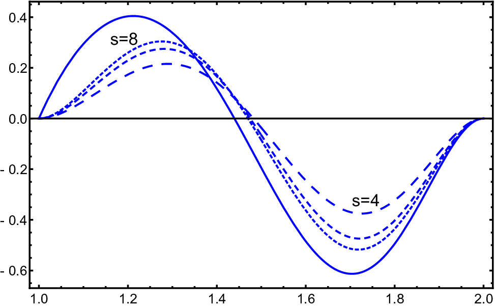
The anomalous dimensions of the singlet currents as a function of dimension $d=2\mu$ for few lower spins are shown in Fig. 3. The LO anomalous dimensions are positive in the whole interval $2<d<4$ while the NLO correction change the sign near $d=3$ . It explains a relative smallness of NLO corrections in $d=3$ .

4 $d=3$ reduction and higher-spin masses

In three dimensions the results can be considerably simplified. First of all,

\displaystyle\eta_{1}

\displaystyle=\frac{8}{3\pi^{2}}\,,

\displaystyle\eta

\displaystyle=\frac{\eta_{1}}{N}\left(1-\frac{8}{3N}\eta_{1}+\ldots\right)\,.

(36)

After some simplifications we obtain for the non-singlet anomalous dimensions in three dimensions

	$\displaystyle\gamma_{\text{ns},1}(s)$	$\displaystyle=-\frac{3}{\left(4s^{2}-1\right)}\,,$
	$\displaystyle\gamma_{\text{ns},2}(s)$	$\displaystyle=\frac{3}{4\left(4s^{2}-1\right)}\Biggr\{-\frac{128s^{2}}{9}-6\pi(-1)^{s}s+\frac{11}{2s-1}-\frac{6}{(2s-1)^{2}}-\frac{3}{2s+1}+\frac{6}{(2s+1)^{2}}+\frac{158}{9}$
		$\displaystyle\qquad\qquad\qquad\qquad-32\log(2)+6sS_{1}\left(\frac{s}{2}-\frac{1}{4}\right)-6sS_{1}\left(\frac{s}{2}-\frac{3}{4}\right)-16S_{1}\left(s-\frac{1}{2}\right)\Biggr\}.$

For the anomalous dimensions of the singlet currents we have

	$\displaystyle\gamma_{1}(s)$	$\displaystyle=\frac{2(s-2)}{2s-1}\,,$
	$\displaystyle\gamma_{2}(s)$	$\displaystyle=\frac{3}{4s^{2}-1}\bigg(-\frac{32s^{2}}{9}-\frac{\left(13s^{2}+14s+6\right)\log(2)}{s}-\frac{3}{2}\pi s+\frac{3}{2}s\left(S_{1}\left(\frac{s}{2}+\frac{3}{4}\right)-S_{1}\left(\frac{s}{2}+\frac{1}{4}\right)\right)$
		$\displaystyle\quad+\frac{3(-1-s+s^{2})}{s}\left(S_{1}\left(\frac{s}{2}\right)-S_{1}\left(\frac{s+1}{2}\right)-S_{1}(s+1)\right)-\frac{(s+2)(7s+6)}{2s}S_{1}\left(s-\frac{1}{2}\right)$
		$\displaystyle\quad+\frac{\left(13s^{2}+3s+3\right)}{s}S_{1}(s)+13s-\frac{9}{s+1}+\frac{1}{2s-1}-\frac{6}{(2s-1)^{2}}-\frac{3}{2s+1}+\frac{9}{2s+3}-\frac{9}{s}+\frac{152}{9}\bigg).$

It may be interesting to compare the results of the large- $N$ expansion with the perturbative results in $4-2\epsilon$ dimensions for $\epsilon=\tfrac{1}{2}$ , which is displayed on Fig. 4 for the $s=4$ current. We see that as $N$ increases the two approximation converge to each other.

Now we can write down the effective masses of higher-spin fields in $AdS_{4}$ :

\displaystyle\begin{aligned} \delta m_{s}^{2}=&\frac{2}{N}(s-2)\eta_{1}+\frac{\eta_{1}^{2}}{N^{2}}\frac{3}{2s+1}\bigg\{-\frac{\left(13s^{2}+14s+6\right)\log(2)}{s}+\frac{\left(13s^{2}+3s+3\right)}{s}S_{1}(s)\\ &-\frac{(s+2)(7s+6)}{2s}S_{1}\left(s-\frac{1}{2}\right)-\frac{32s^{2}}{9}+\frac{41s}{3}-\frac{9}{s+1}-\frac{3}{2s+1}+\frac{9}{2s+3}-\frac{9}{s}\\ &+\frac{137}{9}-\frac{3}{2}\pi s+\frac{3\left(s^{2}-s-1\right)}{s}\left(S_{1}\left(\frac{s}{2}\right)-S_{1}\left(\frac{s+1}{2}\right)-S_{1}(s+1)\right)\\ &+\frac{3}{2}s\left(S_{1}\left(\frac{s}{2}+\frac{3}{4}\right)-S_{1}\left(\frac{s}{2}+\frac{1}{4}\right)\right)\bigg\}.\end{aligned}

(37)

The order- $1/N$ correction is linear, while the effective mass up to the order- $1/N^{2}$ can be written as

\displaystyle\delta m_{s}^{2}

\displaystyle=2\eta(s-2)\big(1+\eta\varkappa(s)+\ldots\big).

(38)

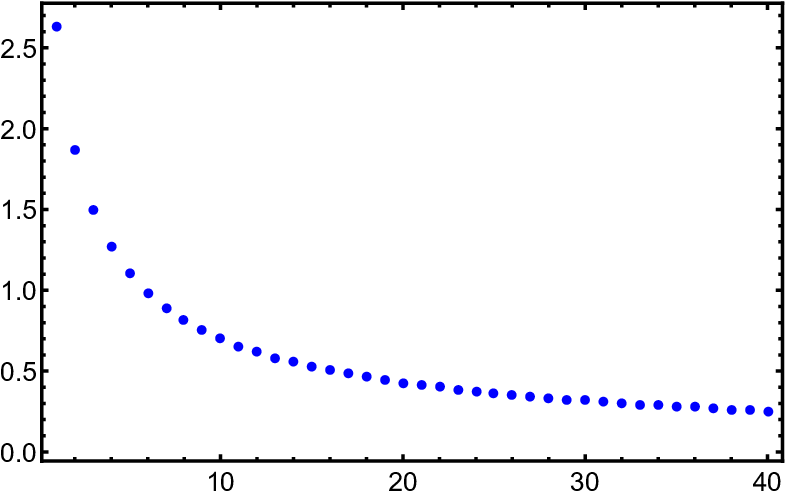
At large spin $\varkappa(s)=\tfrac{39}{8}\frac{\log s}{s}+...$ and we also plot $\varkappa(s)$ in Fig. 5.

5 Summary

We have calculated the $1/N^{2}$ corrections to the anomalous dimensions of the singlet higher-spin currents in the $O(N)$ vector model. Also, using the results of Ref. [43] we recovered the four-loop anomalous dimensions in the $O(N)$ model and checked that the $1/N$ and $\epsilon$ expansions for the anomalous dimensions are in complete agreement with each other.

The $1/N^{2}$ expression for the anomalous dimensions (29) is rather involved but simplifies considerably in three dimensions. We have also related them to the two-loop radiative corrections to the masses of higher-spin fields.

It has been known that the LO critical dimensions of the singlet higher-spin currents coincide in the $O(N)$ and Gross-Neveu models with some identification of the expansion parameters. Our result shows that it is no longer true at the NLO order even in $d=3$ . This also implies that the NLO anomalous dimensions of the higher-spin currents in Chern-Simons matter theories have a more complicated form than the one observed at the LO.

Acknowledgments

We are grateful to Johan Henriksson for spotting two typos in the formulas. This work was supported by Deutsche Forschungsgemeinschaft (DFG) with the grants MO 1801/1-2 (A.M.) and SFB/TRR 55 (M.S.) and in part by the Russian Science Foundation grant 14-42-00047 in association with Lebedev Physical Institute and by the DFG Transregional Collaborative Research Centre TRR 33 and the DFG cluster of excellence “Origin and Structure of the Universe” (E.Sk.).

Appendices

Appendix A Numerical Values

We collect below numerical values of the order- $1/N^{2}$ anomalous dimensions of the singlet currents. It is worth stressing that $\eta_{1}=\frac{8}{3\pi^{2}}$ is the same for the Gross-Neveu and for the critical vector models. It is convenient to give anomalous dimensions as multiples of $(\eta_{1})^{2}$ , see Eq. (22). Conservation of the $O(N)$ - current implies $\gamma_{\text{ns}}(1)=0$ and we obtain for a few lowest spins

\displaystyle\begin{aligned} \gamma_{\text{ns},2}(2)&=-\frac{696}{125}\approx-5.568\,,&\gamma_{\text{ns},2}(3)&=-\frac{263104}{128625}\approx-2.04551\,,\\ \gamma_{\text{ns},2}(4)&=-\frac{548936}{138915}\approx-3.9516\,,&\gamma_{\text{ns},2}(5)&=-\frac{8406592}{3773385}\approx-2.22786\,.\end{aligned}

(A.39)

Conservation of the stress-tensor implies $\gamma(2)=0$ and we have

\displaystyle\begin{aligned} \gamma_{2}(4)&=-\frac{1544}{3087}\approx-0.500162\,,&\gamma_{2}(6)&=-\frac{233008}{259545}\approx-0.897756\,,\\ \gamma_{2}(8)&=-\frac{22279496}{19144125}\approx-1.16378\,,&\gamma_{2}(10)&=-\frac{248880040436}{183833374725}\approx-1.35383\,.\end{aligned}

(A.40)

Let us note that the numerical values for the singlet currents are by an order of magnitude smaller than those in the Gross-Neveu model. Let us also write down the singlet anomalous dimensions in a way that makes it clear that the second order corrections are relatively small

\displaystyle\begin{aligned} \gamma_{2}(4)&=\frac{4}{7}\frac{\eta_{1}}{N}\left(1-0.2364\frac{1}{N}+\ldots\right),&\gamma_{2}(6)&=\frac{8}{11}\frac{\eta_{1}}{N}\left(1-0.3335\frac{1}{N}+\ldots\right),\\ \gamma_{2}(8)&=\frac{4}{5}\frac{\eta_{1}}{N}\left(1-0.3930\frac{1}{N}+\ldots\right),&\gamma_{2}(10)&=\frac{16}{19}\frac{\eta_{1}}{N}\left(1-0.4343\frac{1}{N}+\ldots\right).\end{aligned}

(A.41)

Appendix B Diagrams

In this appendix we collect the results for the diagrams shown in Fig. 2. The expressions below give the divergent part of diagrams with subtracted counterterms. The symmetry factors are already included in these expressions. We obtained for the diagrams $D_{k}$ , $k=1,\ldots,9$

$\displaystyle D_{1}$	$\displaystyle=\frac{\eta_{1}^{2}}{4}\gamma_{\text{ns},1}(s)\Delta\gamma_{1}(s)\,\Biggl(-\frac{1}{6\Delta^{2}}+\frac{1}{3\Delta}\biggl[-1+\frac{1}{\mu+s-1}+\frac{1}{\mu+s-2}$
	$\displaystyle\quad\hskip 113.81102pt+\psi(2\mu-3+s)+\psi(3-\mu)-\psi(\mu-2)-\psi(2)\biggr]\Biggr)\,,$
$\displaystyle D_{2}$	$\displaystyle=\frac{\eta_{1}^{2}}{12}\gamma_{\text{ns},1}(s)\Delta\gamma_{1}(s)\,\Biggl(-\frac{1}{\Delta^{2}}+\frac{1}{\Delta}\biggl[-1+\frac{1}{\mu+s-1}+\frac{1}{\mu+s-2}-\frac{1}{\mu-2}+\psi(2)-\psi(s+1)\biggr]\Biggr)\,,$
$\displaystyle D_{3}$	$\displaystyle=\frac{\eta_{1}^{2}}{32}\Delta\gamma^{2}_{1}(s)\,\Biggl(-\frac{1}{\Delta^{2}}+\frac{2}{\Delta}\biggl[-1+\frac{1}{\mu+s-1}+\frac{1}{\mu+s-2}$
	$\displaystyle\quad\hskip 113.81102pt+\psi(2\mu+s-3)-\psi(s+1)-\psi(\mu-1)+\psi(3-\mu)\biggr]\Biggr)\,,$
$\displaystyle D_{4}$	$\displaystyle=-\frac{1}{\Delta}\,\frac{\eta_{1}^{2}}{16}\,\Delta\gamma^{2}_{1}(s)\,\frac{(s+\mu-1)(s+\mu-2)}{(2-\mu)s(s+2\mu-3)}\,\Phi(j_{s})\,,$
$\displaystyle D_{5}$	$\displaystyle=-\frac{1}{6\Delta}\eta^{2}_{1}\,\Delta\gamma_{1}(s)\,\frac{\mu(\mu-1)(3-\mu)}{\mu-2}\biggl(\psi(\mu+s-1)-\psi(\mu-2)\biggr)\,,$
$\displaystyle D_{6}$	$\displaystyle=-\frac{1}{6\Delta}\eta_{1}^{2}\Delta\gamma_{1}(s)\,\frac{\mu(\mu-1)}{2-\mu}\Biggl(\frac{1}{2-\mu}+\frac{(s+1)(s+2\mu-4)}{s(s+2\mu-3)}\times\Phi(j_{s})\Biggr),$
$\displaystyle D_{7}$	$\displaystyle=D_{8}=-\frac{\eta_{1}^{2}}{4\Delta}\gamma_{\text{ns},1}(s)\Delta\gamma_{1}(s)\frac{(2\mu-3)(s+\mu-1)(s+\mu-2)}{(2-\mu)s(2+2\mu-3)}\,\Phi(j_{s})\,.$	(B.42)

For the last diagram we get

$\displaystyle D_{9}$	$\displaystyle=-\frac{\eta_{1}^{2}}{5\Delta}\Delta\gamma_{1}(s)\frac{\mu(\mu-1)(2\mu-3)}{(2-\mu)^{2}}\Biggl\{-\frac{2\mu-3}{s(s+2\mu-3)}\left(\Psi(j_{s})+\frac{1}{s+2\mu-3}+\frac{1}{2-\mu}-R(\mu)\right)$
	$\displaystyle\quad+\frac{\Gamma(2\mu-2)\Gamma(s)}{\Gamma(s+2\mu-2)}\biggl(S(j_{s})-\psi(s+1)+\psi(1)-\frac{1}{2\mu-3}+\frac{1}{s+2\mu-3}+\frac{1}{2-\mu}-R(\mu)\biggr)$
	$\displaystyle\quad+\frac{\Gamma(2\mu-2)}{\Gamma(\mu-2)\Gamma(s+\mu-1)}\sum_{m=0}^{s-1}C^{s-1}_{m}\frac{\Gamma(s-m)\Gamma(\mu-1+m)\Gamma(s+\mu-2-m)}{(m+1)^{2}\Gamma(s+2\mu-3-m)}\Biggl\}\,.$	(B.43)

Appendix C Vertex and self-energy corrections

In this Appendix we discuss the calculation of the self-energy and vertex corrections diagrams. In total there are eight different diagrams which arise from the SE and vertex corrections to the LO pure singlet diagram. The calculation of SE diagrams is rather straightforward but cumbersome while the vertex corrections could be rather involved. The reason for this is that the diagrams with vertex corrections contain, evidently, divergent subgraph and, therefore, one cannot remove the regulator $\Delta$ from the $\sigma$ lines and use the uniqueness property of the $\sigma\varphi^{2}$ vertex. However it is helpful to take into account that the model under consideration is a conformal one. The form of two- and three- point correlators in CFT is fixed up to normalization factors by the scaling dimensions of the fields. Namely, the dressed (full) propagators and 1PI irreducible three point function $\Gamma_{\sigma\varphi\varphi}$ have the form

\displaystyle D_{\varphi}(x)={\widehat{A}}/{x^{2\Delta_{\varphi}}}\,,

\displaystyle D_{\sigma}(x)={\widehat{B}}/{x^{2\Delta_{\sigma}}}\,,

(C.44)

and

\displaystyle\gamma_{R}(z,x,y)\equiv\Gamma_{\sigma\varphi\varphi}(z,x,y)=\widehat{Z}(z-x)^{-2\alpha}(z-y)^{-2\alpha}(x-y)^{-2\beta}\,.

(C.45)

Here

	$\displaystyle\Delta_{\varphi}$	$\displaystyle=\mu-1+\gamma_{\varphi}\,,$	$\displaystyle\Delta_{\sigma}$	$\displaystyle=2+\gamma_{\sigma}\,,$
	$\displaystyle\alpha$	$\displaystyle=\mu-1-\gamma_{\sigma}/2\,,$	$\displaystyle\beta$	$\displaystyle=2-\gamma_{\varphi}+\gamma_{\sigma}/2\,.$		(C.46)

The explicit expressions for the factors $\widehat{A},~\widehat{B},~\widehat{Z}$ at the order- $1/N$ can be found in Ref. [24]. One can use this information in order to avoid a tedious calculation of the individual diagrams. Namely, it was shown in [24] that the contribution to the anomalous dimension at the $1/N^{2}$ order due to the SE and vertex corrections to the $1/N$ diagram can be extracted from the same diagram with the dressed propagators and vertices.

Let us consider a logarithmically divergent diagram. For such a diagram the number of $\varphi$ lines is equal to the number of basic vertices and twice a number of the $\sigma$ lines,

\displaystyle N_{\varphi}=N_{V}=2N_{\sigma}\,.

(C.47)

Replacing propagators and vertices by full propagators and vertices one gets a superficially divergent diagram. It has to be regularized by introducing the regulator $\Delta$ in any line. The resulting diagram has a simple pole in $\Delta$

\displaystyle G=\frac{1}{\Delta}R+F\,.

(C.48)

The contribution to the anomalous dimension which comes from SE and vertex corrections diagram is equal to

\displaystyle\delta\gamma^{SE+V}=-{2r^{(1)}}/{N^{2}}\,,

(C.49)

where $r^{(1)}$ comes from the expansion of the residue $R$ in $1/N$ , $R=r^{(0)}/N+r^{(1)}/N^{2}+O(1/N^{3})$ .

The triple vertices in the modified diagram has the uniqueness property that usually simplifies calculation greatly. Moreover, it is not necessary to replace all vertices and propagators at once. The contributions from lines and vertices are additive [24]. One can replace a subset of lines and vertices, $S_{1}\subset S$ , satisfying the condition (C.47), calculate the corresponding diagram $G^{(1)}$ and find the coefficient $r^{(1)}_{1}$ . Then the same can be done for the next subset, $S_{2}$ , and so on. If sets $S_{k}$ are not intersecting, $\bigcap_{k}S_{k}=\emptyset$ and $\bigcup_{k}S_{k}=S$ , then $\delta\gamma=-\frac{2}{N^{2}}\sum_{k}r_{k}^{(1)}$ . If the sets $S/\bigcup_{k}S_{k}=S_{+}$ and $\bigcap_{k}S_{k}=S_{-}$ are not empty then we have to add the contributions from the elements in $S_{+}$ and subtract those in $S_{-}$ . We illustrate this rule on the example of the pure singlet diagram, Fig. 1. The corresponding decomposition is shown in Fig. 6.

In the leftmost diagram we replaced two left vertices, the left $\sigma$ line and two horizontal $\varphi$ lines. In the middle diagram – two right vertices, the right $\sigma$ line and the two horizontal $\varphi$ lines. So the contribution of the horizontal lines is counted twice. Thus we have to add the contribution from the lines attached to the operator vertex and subtract contribution from the horizontal lines. It is done by adding the rightmost diagram. All the diagrams are superficially divergent and have to be regularized by shifting index of one of the $\sigma-$ lines by $\Delta$ . All these diagrams (first two are obviously equal each other) can be easily calculated with the help of a chain integration rule and the star-triangle relation.

After simple calculation we find for the residue $r^{(1)}$ of a simple pole of the diagrams $D_{10}$ , $D_{11}$ and $D_{12}$ :

$\displaystyle r^{(1)}_{D_{10}}$	$\displaystyle=r^{(1)}_{D_{11}}=-\frac{1}{2}\eta_{1}\Delta\gamma_{1}(s)\Biggl\{\chi_{1}\left(\psi(\mu+s-1)-\psi(\mu-2)-\frac{\mu}{\mu-1}\right)$
	$\displaystyle\quad+\frac{1}{2}\gamma_{\sigma,1}\left(\psi(s+1)+\psi(s+2\mu-3)-2\psi(1)+\psi(3-\mu)-\psi(\mu-1)+6\frac{3-\mu}{\mu-2}\right)$
	$\displaystyle\quad+\eta_{1}\left[\frac{2\mu^{2}-3\mu+2}{\mu-2}\cdot R(\mu)+2(\mu-1)\left(4-\frac{7}{(\mu-2)^{2}}\right)\right]\Biggr\},$	(C.50)

where $\chi=-\eta-\gamma_{\sigma}=\chi_{1}/N+O(1/N^{2})$ and

	$\displaystyle r^{(1)}_{D_{12}}$	$\displaystyle=-\frac{1}{4}\eta_{1}^{2}\Delta\gamma_{1}(s)\Biggl\{2\Big(\psi(s+\mu-2)-\psi(\mu-1)+1\Big)$
		$\displaystyle\quad+\psi(\mu-1)-\psi(3-\mu)-\psi(s+2\mu-3)+\psi(s+1)\Biggr\}.$		(C.51)

References

(1) J. Zinn-Justin, Quantum field theory and critical phenomena, vol. 77. 1989.
(2) E. Brézin, J. C. Le Guillou, J. Zinn-Justin and B. G. Nickel, Higher order contributions to critical exponents, Phys. Lett. A44 (1973) 327.
(3) D. I. Kazakov, O. V. Tarasov and A. A. Vladimirov, Calculation of Critical Exponents by Quantum Field Theory Methods, Sov. Phys. JETP 50 (1979) 521.
(4) F. M. Dittes, Yu. A. Kubyshin and O. V. Tarasov, Four Loop Approximation in the phi**4 Model, Theor. Math. Phys. 37 (1979) 879.
(5) K. G. Chetyrkin, A. L. Kataev and F. V. Tkachov, Five Loop Calculations in the $g\phi^{4}$ Model and the Critical Index $\eta$ , Phys. Lett. B99 (1981) 147.
(6) S. G. Gorishnii, S. A. Larin, F. V. Tkachov and K. G. Chetyrkin, Five Loop Renormalization Group Calculations in the $g\phi^{4}$ in Four-dimensions Theory, Phys. Lett. B132 (1983) 351.
(7) H. Kleinert, J. Neu, V. Schulte-Frohlinde, K. G. Chetyrkin and S. A. Larin, Five loop renormalization group functions of O(n) symmetric phi**4 theory and epsilon expansions of critical exponents up to epsilon**5, Phys. Lett. B272 (1991) 39–44, [hep-th/9503230].
(8) M. V. Kompaniets and E. Panzer, Minimally subtracted six loop renormalization of $O(n)$ -symmetric $\phi^{4}$ theory and critical exponents, 1705.06483.
(9) A. N. Vasiliev, Yu. M. Pismak and Yu. R. Khonkonen, 1/n expansion: calculation of the exponent eta in the order 1/n**3 by the conformal bootstrap method, Theor. Math. Phys. 50 (1982) 127–134.
(10) A. N. Vasiliev, S. E. Derkachov, N. A. Kivel and A. S. Stepanenko, The 1/n expansion in the Gross-Neveu model: Conformal bootstrap calculation of the index eta in order 1/n**3, Theor. Math. Phys. 94 (1993) 127–136.
(11) J. A. Gracey, Computation of critical exponent eta at O(1/N**3) in the four Fermi model in arbitrary dimensions, Int. J. Mod. Phys. A9 (1994) 727–744, [hep-th/9306107].
(12) A. N. Vasilev, The field theoretic renormalization group in critical behavior theory and stochastic dynamics. 2004.
(13) I. R. Klebanov and A. M. Polyakov, AdS dual of the critical $O(N)$ vector model, Phys. Lett. B550 (2002) 213–219, [hep-th/0210114].
(14) E. Sezgin and P. Sundell, Massless higher spins and holography, Nucl.Phys. B644 (2002) 303–370, [hep-th/0205131].
(15) E. Sezgin and P. Sundell, Holography in 4D (super) higher spin theories and a test via cubic scalar couplings, JHEP 0507 (2005) 044, [hep-th/0305040].
(16) R. G. Leigh and A. C. Petkou, Holography of the N=1 higher spin theory on AdS(4), JHEP 0306 (2003) 011, [hep-th/0304217].
(17) S. Giombi and X. Yin, Higher Spin Gauge Theory and Holography: The Three-Point Functions, JHEP 09 (2010) 115, [0912.3462].
(18) S. Giombi and I. R. Klebanov, One Loop Tests of Higher Spin AdS/CFT, JHEP 12 (2013) 068, [1308.2337].
(19) S. Giombi, I. R. Klebanov and A. A. Tseytlin, Partition Functions and Casimir Energies in Higher Spin AdS_d+1/CFT_d, Phys. Rev. D90 (2014) 024048, [1402.5396].
(20) L. Girardello, M. Porrati and A. Zaffaroni, 3-D interacting CFTs and generalized Higgs phenomenon in higher spin theories on AdS, Phys. Lett. B561 (2003) 289–293, [hep-th/0212181].
(21) R. Manvelyan, K. Mkrtchyan and W. Ruhl, Ultraviolet behaviour of higher spin gauge field propagators and one loop mass renormalization, Nucl. Phys. B803 (2008) 405–427, [0804.1211].
(22) E. D. Skvortsov, On (Un)Broken Higher-Spin Symmetry in Vector Models, in Proceedings, International Workshop on Higher Spin Gauge Theories: Singapore, Singapore, November 4-6, 2015, pp. 103–137, 2017, hep-th/1512.05994.
(23) K. Lang and W. Ruhl, The Critical $O(N)$ sigma model at dimension $2<d<4$ and order 1/n**2: Operator product expansions and renormalization, Nucl. Phys. B377 (1992) 371–401.
(24) S. E. Derkachov and A. N. Manashov, The Simple scheme for the calculation of the anomalous dimensions of composite operators in the 1/N expansion, Nucl. Phys. B522 (1998) 301–320, [hep-th/9710015].
(25) S. Giombi, S. Minwalla, S. Prakash, S. P. Trivedi, S. R. Wadia and X. Yin, Chern-Simons Theory with Vector Fermion Matter, Eur. Phys. J. C72 (2012) 2112, [1110.4386].
(26) O. Aharony, G. Gur-Ari and R. Yacoby, d=3 Bosonic Vector Models Coupled to Chern-Simons Gauge Theories, JHEP 03 (2012) 037, [1110.4382].
(27) J. Maldacena and A. Zhiboedov, Constraining conformal field theories with a slightly broken higher spin symmetry, 1204.3882.
(28) O. Aharony, G. Gur-Ari and R. Yacoby, Correlation Functions of Large N Chern-Simons-Matter Theories and Bosonization in Three Dimensions, JHEP 12 (2012) 028, [1207.4593].
(29) T. Muta and D. S. Popovic, Anomalous Dimensions of Composite Operators in the Gross-Neveu Model in Two + Epsilon Dimensions, Prog. Theor. Phys. 57 (1977) 1705.
(30) S. Giombi, V. Gurucharan, V. Kirilin, S. Prakash and E. Skvortsov, On the Higher-Spin Spectrum in Large N Chern-Simons Vector Models, JHEP 01 (2017) 058, [1610.08472].
(31) A. N. Manashov and E. D. Skvortsov, Higher-spin currents in the Gross-Neveu model at 1/n², JHEP 01 (2017) 132, [1610.06938].
(32) K. G. Wilson and M. E. Fisher, Critical exponents in 3.99 dimensions, Phys. Rev. Lett. 28 (1972) 240–243.
(33) K. G. Wilson and J. B. Kogut, The Renormalization group and the epsilon expansion, Phys. Rept. 12 (1974) 75–200.
(34) A. N. Vasiliev and M. Yu. Nalimov, Analog of Dimensional Regularization for Calculation of the Renormalization Group Functions in the 1/n Expansion for Arbitrary Dimension of Space, Theor. Math. Phys. 55 (1983) 423–431.
(35) A. N. Vasiliev and A. S. Stepanenko, A Method of calculating the critical dimensions of composite operators in the massless nonlinear sigma model, Theor. Math. Phys. 94 (1993) 471–481.
(36) S. E. Derkachov and A. N. Manashov, Critical dimensions of composite operators in the nonlinear sigma model, Theor. Math. Phys. 116 (1998) 1034–1049.
(37) A. N. Vasiliev, M. Pismak, Yu and Yu. R. Khonkonen, Simple Method of Calculating the Critical Indices in the 1/ $N$ Expansion, Theor. Math. Phys. 46 (1981) 104–113.
(38) A. N. Vasiliev, Yu. M. Pismak and Yu. R. Khonkonen, 1/ $N$ Expansion: Calculation of the Exponents $\eta$ and Nu in the Order 1/ $N^{2}$ for Arbitrary Number of Dimensions, Theor. Math. Phys. 47 (1981) 465–475.
(39) L. F. Alday, A. Bissi and T. Lukowski, Large spin systematics in CFT, JHEP 11 (2015) 101, [1502.07707].
(40) L. F. Alday and A. Zhiboedov, An Algebraic Approach to the Analytic Bootstrap, JHEP 04 (2017) 157, [1510.08091].
(41) Yu. L. Dokshitzer, G. Marchesini and G. P. Salam, Revisiting parton evolution and the large-x limit, Phys. Lett. B634 (2006) 504–507, [hep-ph/0511302].
(42) B. Basso and G. P. Korchemsky, Anomalous dimensions of high-spin operators beyond the leading order, Nucl. Phys. B775 (2007) 1–30, [hep-th/0612247].
(43) S. E. Derkachov, J. A. Gracey and A. N. Manashov, Four loop anomalous dimensions of gradient operators in phi**4 theory, Eur. Phys. J. C2 (1998) 569–579, [hep-ph/9705268].

DESY 17 – 095 LMU-ASC 36/17 Higher spin currents in the critical O⁡(N)O(N) vector model at 1/N21/N^{2}