Good Clusterings Have Large Volume

In Section $2$, we introduce some notation and review related work. We then use the known vertex characterization of [7] as a starting point for the new contributions in this paper. We briefly outline these contributions in the following paragraphs. Section $3$ is a complete and self-contained presentation of our results. Section $4$ contains the necessary proofs. We conclude our discussion with some final remarks in Section $5$. Parts of this work are based on the first author’s Ph.D. dissertation ([11]) and the second author’s M.Sc. thesis ([23]).

Let throughout this paper $n,d,k\in\mathbb{N}:=\{1,2,\dots\}$ be fixed. Let $X:=\{x_{1},\dots,x_{n}\}\subseteq\mathbb{R}^{d}$ be a set of $n$ distinct non-zero data points and for $m\in\mathbb{N}$ define $[m]:=\{1,\dots,m\}$. We call a partition $C:=(C_{1},\dots,C_{k})$ of $X$ a clustering and call $\left|C\right|:=(\left|C_{1}\right|,\dots,\left|C_{k}\right|)$ its shape. For $i\in[k]$, we call $C_{i}$ the $i$-th cluster of $C$ and $\left|C_{i}\right|$ its size. Let $s^{-}:=(s^{-}_{1},\dots,s^{-}_{k})$, $s^{+}:=(s_{1}^{+},\dots,s_{k}^{+})\in\mathbb{N}^{k}$ such that $0\leq s^{-}_{i}\leq s^{+}_{i}\leq n$ for all $i\in[k]$ be the lower and upper bounds on the cluster sizes.

A clustering $C$ is said to be feasible if it satisfies $s^{-}\leq\left|C\right|\leq s^{+}$ componentwisely. We will only consider feasible clusterings in this paper. $C$ is called separable if all pairs of clusters are linearly separable, i.e. for all $i,j\in[k]$, $i\not=j$ there is $a_{ij}\in\mathbb{R}^{d}$ and $\gamma_{ij}\in\mathbb{R}$ such that $a_{ij}^{T}x\leq\gamma_{ij}\leq a_{ij}^{T}y$ for all $x\in C_{i}$, $y\in C_{j}$. The hyperplane separating the clusters is denoted by $H_{(a_{ij},\gamma_{ij})}:=\{x\in\mathbb{R}^{d}\,|\,a_{ij}^{T}x=\gamma_{ij}\}$. Analogously, we define $H^{\leq}_{(a_{ij},\gamma_{ij})}$ and $H^{\geq}_{(a_{ij},\gamma_{ij})}$ to be the respective half-spaces. A constrained least-squares assignment (LSA) for a given set of sites $a_{1},\dots,a_{k}\in\mathbb{R}^{d}$ is a clustering $C=(C_{1},\dots,C_{k})$ minimizing

over all clusterings with the same shape as $C$. If $C$ minimizes (1) over all feasible clusterings, we say $C$ is a (general) LSA. We call $a=(a_{1}^{T},\dots,a_{k}^{T})^{T}\in\mathbb{R}^{d\cdot k}$ the site vector.

Recall that power diagrams are a generalization of the well-known Voronoi diagrams (see [3]). There are several equivalent definitions of power diagrams. We briefly recall the definition that is best for our purposes (see [12]). Let $a:=(a_{1}^{T},\dots,a_{k}^{T})^{T}\in\mathbb{R}^{d\cdot k}$ be a site vector with distinct sites $a_{1},\dots,a_{k}\in\mathbb{R}^{d}$ and let $\alpha_{1},\dots,\alpha_{k}\in\mathbb{R}$. For $i\in[k]$, we call

the $i$-th cell of the power diagram $(P_{1},\dots,P_{k})$.

[4] showed the following connection between constrained LSAs and power diagrams: If $C$ is a constrained LSA to the site vector $a$, then there is a power diagram with site vector $a$ satisfying $C_{i}\subseteq\operatorname{int}(P_{i})$ for all $i\in[k]$. On the other hand, if a power diagram $(P_{1},\dots,P_{k})$ with site vector $a$ satisfies $C_{i}\subseteq P_{i}$ for all $i\in[k]$, then $C$ is a constrained LSA to the site vector $a$. If $C_{i}\subseteq P_{i}$ for all $i\in[k]$, we say the power diagram induces the clustering and call it a separating power diagram.

In order to compare two clusterings $C:=(C_{1},\dots,C_{k})$, $C^{\prime}:=(C^{\prime}_{1},\dots,C^{\prime}_{k})$, we define the clustering difference graph (CDG) to be the labeled directed multigraph $CDG(C,C^{\prime}):=(V,E)$ with node set $V:=[k]$ and edge set $E$ constructed as follows: For each $x_{j}\in C_{i}\cap C^{\prime}_{l}$ with distinct $i,l\in[k]$, there is an edge $(i,l)\in E$ with label $x_{j}$. W.l.o.g. we delete isolated nodes in the CDG, since these would correspond to clusters that are identical in $C$ and $C^{\prime}$. We can derive $C^{\prime}$ from $C$ by applying operations corresponding to the edges of $CDG(C,C^{\prime})$.

Let $(i_{1},i_{2})-(i_{2},i_{3})-\cdots-(i_{t},i_{t+1})$ be an edge path in $CDG(C,C^{\prime})$ with labels $x_{j_{1}},\dots,x_{j_{t}}$. Applying the movement

to $C$ means deriving the clustering $\bar{C}=(\bar{C}_{1},\dots,\bar{C}_{k})$ by setting $\bar{C}_{i_{l}}:=(C_{i_{l}}\setminus\{x_{j_{l}}\})\cup\{x_{j_{l-1}}\}$ for all $l\in\{2,\dots,t\}$, $\bar{C}_{i_{1}}:=C_{i_{1}}\setminus\{x_{j_{1}}\}$, $\bar{C}_{i_{t+1}}:=C_{i_{t+1}}\cup\{x_{j_{t}}\}$ and $\bar{C}_{r}:=C_{r}$ for all $r\in[k]\setminus\{i_{1},\dots,i_{t+1}\}$.

If $i_{t+1}=i_{1}$, i.e. in case of a cycle, we speak of a cyclical movement. We then obtain $\bar{C}_{i_{1}}=\bar{C}_{i_{t+1}}:=(C_{i_{1}}\setminus\{x_{j_{1}}\})\cup\{x_{j_{t}}\}$ and all cluster sizes remain the same. The inverse (cyclical) movement $M^{-1}$ is defined via the corresponding path (cycle) $(i_{t+1},i_{t})-(i_{t},i_{t-1})-\cdots-(i_{2},i_{1})$ in $CDG(C^{\prime},C)$. Clearly, one can obtain any clustering from any other clustering by (greedily) decomposing their clustering difference graph into paths and cycles and applying the corresponding (cyclical) movements to $C$. If $\left|C\right|=\left|C^{\prime}\right|$, then $CDG(C,C^{\prime})$ decomposes into cycles, i.e. cyclical movements suffice to transform $C$ into $C^{\prime}$, c.f. [11].

Figures 2 and 3 depict a clustering of twelve data points in $\mathbb{R}^{2}$ with $C_{1}$ black, $C_{2}$ blue, $C_{3}$ red, as well as two clusterings which can be derived from it by applying a movement (Figure 2) and a cyclical movement (Figure 3), respectively.

The polytope we are studying was introduced in [7] and [24]:

For a clustering $C=(C_{1},\dots,C_{k})$ and $i\in[k]$, let $\sigma_{i}:=\sum\limits_{x\in C_{i}}x\in\mathbb{R}^{d}$. The clustering vector of $C$ is $w(C):=(\sigma_{1}^{T},\dots,\sigma_{k}^{T})^{T}\in\mathbb{R}^{d\cdot k}$. Then $\mathcal{P}^{\pm}(X,k,s^{-},s^{+}):=\operatorname{conv}(\{w(C)\ |\ C$ is feasible$\})$ is called the bounded-shape partition polytope. If $s=s^{-}=s^{+}$, then we call $\mathcal{P}^{=}_{s}=\mathcal{P}^{\pm}(X,k,s,s)$ the single-shape partition polytope. Another interesting special case is the all-shape partition polytope $\mathcal{P}$ investigated by [17] which is obtained by choosing $s^{-}=(0,\dots,0)$ and $s^{+}=(n,\dots,n)$. When the bounds are clear from the context, we use the simpler notation $\mathcal{P}^{\pm}=\mathcal{P}^{\pm}(X,k,s^{-},s^{+})$ and $\mathcal{P}^{=}=\mathcal{P}^{=}_{s}$.

Note that $\mathcal{P}^{\pm}$ is a projection of the generalized assignment polytope investigated in [20]. We want to stress that, since these polytopes are defined as a convex hull, we do not have explicit information on (facet-defining) valid inequalities. This will play an important role in our discussion, as we have to study the edge structure of the polytopes (which may have exponential size) in order to construct the normal cones of its vertices. We use the notation $N_{P}(v):=\{a\in\mathbb{R}^{d}\ |\ a^{T}v\geq a^{T}x\ \forall\,x\in P\}$ for the normal cone of $v$ in a polytope $P$.

We observe the following connection between single-shape and bounded-shape partition polytopes.

Note that Lemma 1 implies that every vertex $w(C)$ of $\mathcal{P}^{\pm}$ is also a vertex of $\mathcal{P}^{=}_{\left|C\right|}$ and that $N_{\mathcal{P}^{\pm}}(w(C))\subseteq N_{\mathcal{P}^{=}}(w(C))$ for every clustering vector $w(C)$. [7] gave a first characterization of the vertices of $\mathcal{P}^{\pm}$.

A proof is given in [7] and, with more technical detail, in [24]. We call a clustering corresponding to a vertex of $\mathcal{P}^{\pm}$ a vertex clustering. Condition $3$ states linear separability of the clusters with separation directions $a_{ij}:=a_{j}-a_{i}\in\mathbb{R}^{d}$ and right-hand sides $\gamma_{ij}:=\alpha_{i}-\alpha_{j}$ for all $i,j\in[k]$. This implies the existence of a separating power diagram. This property can alternatively be derived from the observation that computation of an optimal constrained LSA corresponds precisly to linear optimization over the corresponding single-shape partition polytope $\mathcal{P}^{=}$ (see [11]).

If the scalars $\alpha_{1},\dots,\alpha_{k}$ additionally satisfy conditions $1$ and $2$, then the resulting separation fulfills some additional properties. For example, if two clusters satisfy $s^{-}<\left|C_{i}\right|,\left|C_{j}\right|<s^{+}$, then $C_{i}$ and $C_{j}$ are “$0$-separable” (see [5]), in particular they can be separated by a hyperplane containing the origin. Any vector $a\in\operatorname{int}(N_{\mathcal{P}^{\pm}}(w(C)))$ can be chosen to construct suitable $\alpha_{1},\dots,\alpha_{k}$ such that the properties of Proposition 2 are satisfied, c.f. [7].

This gives the following corollary (see [11, 23]).

The statement also holds for the single-shape partition polytope $\mathcal{P}^{=}$ by replacing “$\pm$” by “$=$”. Further, the normal cone of a vertex clustering of the single-shape partition polytope encodes exactly all site vectors that allow a separating power diagram (see [11]). Clearly, if $a$ is in the normal cone, then so is $\lambda a$ for every $\lambda>0$. Thus $a$ and $\lambda a$ yield the same constrained LSA. This was first proven by [4], in a different notation.

Before we turn to our main results, we would like to mention two tools that will make our arguments easier. First, recall our assumption that the zero vector is not contained in $X$. This is no restriction, since the overall structure of a data set is not changed when translating the whole set by the same vector. Second, we can interpret any movement (recall Section 2.2) as a translation of the corresponding clustering vector. Let $C,C^{\prime}$ such that $CDG(C,C^{\prime})$ is a single path or cycle corresponding to a (cyclical) movement $M$. Then the difference of the clustering vectors $w(M):=w(C^{\prime})-w(C)$ is called the vector of the movement $M$. Note that the vector of the inverse movement is given by $w(M^{-1})=-w(M)$.

Note that $d:\mathbb{S}^{d\cdot k}\times\mathbb{S}^{d\cdot k}\mapsto\mathbb{R}$ is a metric, takes values between $0$ and $\pi$, and that an infimum always exists, because $L(\gamma)\geq 0$ for all $\gamma:[0;1]\mapsto\mathbb{R}^{d\cdot k}$.

If a vertex clustering $C$ of $\mathcal{P}^{\pm}$ or $\mathcal{P}^{=}$ has a large normal cone, then a randomly chosen site vector is likely to lie in its cone. By the previous observations, the chosen site vector defines a separating power diagram inducing $C$. We are interested in measuring the volume of the normal cones of the bounded-shape and single-shape partition polytopes in order to characterize “good” clusterings.

We follow the notation of [10] who used the volume of normal cones for the studies of combinatorial diameters. For a cone $K\subseteq\mathbb{R}^{d\cdot k}$, we call $B(K):=K\cap\mathbb{S}^{d\cdot k}$ the base of $K$. The volume of $K$ is then defined as the $(d\cdot k-1)$-dimensional volume of $B(K)$ and is denoted by $\operatorname{vol}(K)$. A set $A\subseteq\mathbb{S}^{d\cdot k}$ is called spherically convex, if for all $x,y\in A$ the geodesic $\gamma:[0;1]\mapsto\mathbb{S}^{d\cdot k}$ connecting $x$ and $y$ with $\gamma(0)=x$ and $\gamma(1)=y$ is contained in $A$. Recall that a geodesic is a curve on the sphere with shortest length. Note that the base of a cone is spherically convex itself. These notions allow us to formally introduce two variants of a new term which we call the volume of a clustering.

The volume of a clustering puts the volume of the respective normal cones in relation to the volume of the whole space, so by definition $\mu_{\pm},\mu_{=}\in[0;1]$. The only difference is that the BHR volume compares the clustering to all feasible clusterings and the LSA volume compares it to all clusterings of the same shape. In the following, we use the simple wording “volume of a clustering” to refer to both variants when they behave analogously.

Note that vol$(\mathbb{R}^{d\cdot k})$ equals the area of the surface of $\mathbb{S}^{d\cdot k}$. In practice, permutations of the clusters/sites yield the same clustering and the respective normal cones have equal volume. For our purposes, it is more useful to consider each permutation as an individual clustering. However, if all cluster bounds are symmetric, then the volume defined above only takes values between 0 and $\frac{1}{k!}$, because it only takes one possible permutation into account. By Lemma 1, $\mu_{\pm}(C)\leq\mu_{=}(C)$ for all clusterings $C$.

The volume of a clustering quantifies the “fraction” of all site vectors of separating power diagrams that induce the given clustering. This is quite a different concept than the two widely used quality measures for clusterings: the least-squares functional, which measures the quadratic Euclidean distance of the data points to their respective site, and the so-called margin, which measures the smallest Euclidean distance of data points to the nearest separating hyperplane (see [12]). Let us exhibit the difference between the LSA volume and the classical measures. (The BHR volume behaves analogously.)

Consider Figure 4, which depicts two similar data sets, where three “point clouds” of the same structure are at different distance to each other. The least-squares values of both clusterings are equal, whereas the right-hand clustering has a larger volume. This can be seen by noting that all power diagrams that induce the left-hand clustering also induce the right-hand one. Conversely, there are many power diagrams that induce the right-hand clustering, but not the left-hand one. This means that the set of site vectors that give the left-hand clustering is a strict subset of the set of site vectors that give the right-hand one. Informally, unlike a least-squares functional, the volume is able to take the distance between different clusters into account.

Now, consider Figure 5. The only difference between the data sets lies in the vertical scaling of the points in the top clusters and the horizontal scaling of the points in the bottom cluster. Both clusterings have equal margin, but the one on the right has a lower volume. It is easy to see that the separating hyperplanes on the right can be perturbed less due to the long, drawn-out clusters. This implies that the site vectors that define a separating power diagram inducing the right-hand clustering is a strict subset of the site vectors for the left-hand clustering. While the margin informally measures the ability to shift the separating hyperplanes closer to the clusters (without changing their directions), the volume measures the ability to perturb the normals of the separating hyperplanes.

Note that it does not matter whether we consider $\mathbb{R}^{d\cdot k}$ or the affine hull of the polytope in Definition 6, because all normal cones have a lineality space $\operatorname{lin}(\mathcal{P}^{\star}-v)^{\perp}$ with $v\in\mathcal{P}^{\star}$ for $\star\in\{\pm,=\}$, respectively. Since we consider the volume of a cone relative to the whole space, we can restrict to the affine hull of the polytopes (see [23] for further details).

In fact, one can show that $\mathcal{P}^{\pm}$ and $\mathcal{P}^{=}$ are contained in a $(d\cdot(k-1))$-dimensional affine subspace. Let $a=(\bar{a}^{T},\dots,\bar{a}^{T})^{T}\in\mathbb{R}^{d\cdot k}$ with $\bar{a}\in\mathbb{R}^{d}$ and consider an arbitrary clustering vector $w(C)$. Then

so $\mathcal{P}^{\star}\subseteq\{x\in\mathbb{R}^{d\cdot k}\ |\ (\bar{a}^{T},\dots,\bar{a}^{T})x=\sum\limits_{j=1}^{n}\bar{a}^{T}x_{j}\}$ for $\star\in\{\pm,=\}$. Thus the dimension is at most $d\cdot k-d=d\cdot(k-1)$.

We conclude the section by showing that the volume of a clustering is well-defined, and by providing an explicit algebraic description.

Note that the coefficient in (2) is the inverse of the area of the surface of $\mathbb{S}^{d\cdot k}$. We postpone the proof of this theorem to Section 4.1.

The closest result in the literature is by [17], who characterized the neighborhood of a vertex $w(C)$ of the all-shape partition polytope $\mathcal{P}$. They showed that edges incident to $w(C)$ correspond to movements of the form $C_{i}\stackrel{{\scriptstyle x}}{{\longrightarrow}}C_{j}$ or $C_{i}\stackrel{{\scriptstyle x}}{{\longrightarrow}}C_{j}\stackrel{{\scriptstyle\nu x}}{{\longrightarrow}}C_{i}$ with $\nu<0$ and $i,j\in[k]$, $i\not=j$. Moreover, they proved that, if $\operatorname{lin}(\{x\})\cap X=\{x\}$ for all $x\in X$ then all edges of $\mathcal{P}$ correspond to movements that move a single element from one cluster to another. The following theorem extends their result to general lower and upper bounds $s^{-}$ and $s^{+}$.

The different cases of Theorem 8 are depicted in Figure 6. Note that the case of two movements can only occur if all sites lie on a line. For the single-shape partition polytope, we obtain the following corollary.

We dedicate Section 4.2 to the proof of this theorem and corollary. Figure 7 shows two vertex clusterings of $\mathcal{P}^{=}$ which are connected by an edge. The site vector of the plotted power diagram lies on the boundary of the normal cones of both vertices. As one can see, the data points on the boundary of the cells, which exist due to Corollary 3, move to the other cell.

Figure 8 illustrates two clusterings of 27 data points in $\mathbb{R}^{2}$. These clusterings were computed by running the $k$-means algorithm 50 times with three random sites in the beginning. In every iteration the $k$-means algorithm computes a LSA to the current sites and updates each site as the arithmetic mean of the points in the cluster. This is repeated until the clustering does not change anymore. Note that the $k$-means algorithm is deterministic, but its result depends on the choice of the initial sites. Whereas the clustering on the left-hand side (except for permutation of the colors) was the output in 25 of the 50 runs, the one on the right-hand side was returned only once. Intuitively, one sees that the left-hand clustering captures the structure of the data better than the one on the right-hand side.

This fits with our quantitative measure: Both volumes of the clustering on the left-hand side are higher ($\mu_{\pm}\approx 0.0076$, $\mu_{=}\approx 0.041$) than the ones of the clustering on the right-hand side ($\mu_{\pm}<0.0001$, $\mu_{=}<0.01$). The volumes of the respective normal cones were computed with MATLAB using the function Volume Computation of Convex Bodies of [14] with an error tolerance of 0.001. The different volumes can also be verified by computing the edges of a respective normal cone and projecting the edges (which are (normalized) site vectors themselves) to their $d$-dimensional components for each of the $k$ sites. Each site of a site vector in the normal cone is located in the convex hull of the corresponding sites of the edges of the normal cone.

Figures 9 and 10 illustrate the three areas of the $2$-dimensional sites for the respective clusterings w.r.t. $\mathcal{P}$ and $\mathcal{P}^{=}$. Because of the invariance of power diagrams under scaling of sites (Proposition 4), we have to choose a fixed scaling of the $6$-dimensional site vectors to obtain a meaningful visualization. Here the site vectors are scaled to Euclidean norm 4.

One sees that the areas on the left-hand side are larger than the ones on the right-hand side, especially for the all-shape partition polytope (Figure 9). Note that these areas do not mean that one can choose three sites arbitrarily within the three areas and obtain an optimal site vector for the respective clustering. Instead, for any arbitrary site within one of these areas, there are sites in the respective other areas such that the corresponding site vector is inside the normal cone of the clustering. Further, these areas contain sites of a representative for all equivalence classes of site vectors in the normal cone. For the single-shape partition polytope, these areas depict representatives of all site vectors for which the respective clusterings are optimal constrained LSAs, see Figure 10.

The BHR and LSA stability, $\tau^{p}_{\pm}$ and $\tau^{p}_{=}$, measure how much we can perturb the site vector $a$ within the respective normal cone w.r.t. the $p$-norm without changing the induced clustering. Of special interest are $p=2,\infty$. Whereas the Euclidean norm weighs the perturbation of all sites equally, the infinity norm considers the highest possible perturbation of one individual site. We highlight the differences after stating our main theorem.

Note that the above definition can be extended to all site vectors by inserting the corresponding representative of the equivalence class into $\tau^{p}_{\star}$, $\star\in\{\pm,=\}$. Geometrically, a “most stable” site vector w.r.t $p$ can be described by dropping a $p$-norm unit ball into the normal cone with $0\in\mathbb{R}^{d\cdot k}$ as gravity center and computing where it gets stuck due to being blocked by the facets of the cone. The center of this unit ball then is a vector which lies “most centrally” within the normal cone. Figure 11 illustrates two examples of this approach.

Minimizing the squared Euclidean norm corresponds to dropping the $p$-norm unit ball into the cone with the origin as gravity center that attracts the ball. The constraints ensure that the ball remains inside the cone. We postpone a proof of the theorem to Section 4.3.

The stability of an optimal solution $z^{(p)}$ of (3) is $\tau^{p}_{\star}(z^{(p)})=\frac{1}{\left\|z^{(p)}\right\|_{2}}$. Problem (3) is a quadratic optimization problem with linear constraints and the auxiliary problems (4) are linear optimization problems over a convex set. The edges $v_{j}$ encode single (cyclical) movements for all $j\in[t]$ (Theorem 8 and Corollary 9). Note that there might be exponentially many edges and, thus, we might have to solve exponentially many auxiliary problems.

Problem (3) models the facets of the normal cone blocking the unit ball. We justify our approach that the ball is blocked by facets, rather than lower-dimensional faces of the cone, with a short example in Section 4.3.

Fix $p\in[1;\infty)$ and let $z^{(p)}:=(z_{1}^{T},\dots,z_{k}^{T})^{T}\in\mathbb{R}^{d\cdot k}$ be an optimal solution of (3). Then we can perturb one site, say $z_{1}\in\mathbb{R}^{d}$, within a $p$-norm ball with radius 1 without changing the clustering. For $0<\delta<k^{-\frac{1}{p}}$ and $\tilde{z}:=(\tilde{z}_{1}^{T},\dots,\tilde{z}_{k}^{T})^{T}\in\mathbb{R}^{d\cdot k}$ with $\tilde{z}_{i}\in\mathbb{B}^{p}_{\delta}(z_{i})\subseteq\mathbb{R}^{d}$ for all $i\in[k]$, we obtain

Thus, $\tilde{z}\in\operatorname{int}(\mathbb{B}^{p}_{1}(z^{(p)}))\subseteq\operatorname{int}(N_{\mathcal{P}^{\star}}(w(C)))$, i.e. we can perturb each site within a $p$-norm ball with e.g. radius $\delta:=(k+1)^{-\frac{1}{p}}<k^{-\frac{1}{p}}$ without changing the clustering.

If $p=\infty$, we can even choose $0<\delta<1$, because then

Next, we show how to obtain a feasible approximate solution of (3). It is well-known that for all $p,q\in[1;\infty]$ there is a positive constant $c_{p,q}>0$ only depending on $p,q$ and the dimension of the space such that $\left\|x\right\|_{p}\leq c_{p,q}\left\|x\right\|_{q}$ for all $x\in\mathbb{R}^{d\cdot k}$.

Note that an upper bound on the objective value of the approximate solution $z^{\prime}$ implies a lower bound on its stability $\tau^{p}_{\star}(z^{\prime})$ and that $d(z^{\prime},z^{(p)})=0$, i.e. $z^{\prime}$ and $z^{(p)}$ define the same separating power diagram. If we choose $p=2$, then the auxiliary problems (4) of Theorem 11 have optimal objective values $\gamma_{j}=-\left\|v_{j}\right\|_{2}$ for all $j\in[t]$. Problem (3) then reduces to

After computing an optimal solution $z^{(2)}$ of (5), we get a site vector $z^{\prime}=c_{2,p}z^{(2)}$ for any arbitrary $p\in[1;\infty]$ whose norm can be bounded from above by the norm of the most stable (w.r.t. $p$) site vector $z^{(p)}$ and a constant factor only depending on $p$ (Theorem 12). Hence, we obtain a provable approximation.

We use Figures 12 – 17 to illustrate computational results for the the two clusterings of Figure 8. We compute the optimal sites (crosses in respective colors), following the programs in Theorem 11, w.r.t. $p=2,\infty$ for the all-shape and single-shape partition polytopes. The $6$-dimensional optimal solutions of (3) were again scaled to Euclidean norm 4. Figures 12 and 13 depict the area of possible perturbation without changing the clustering when only perturbing the first (black) site and keeping the other two sites fixed.

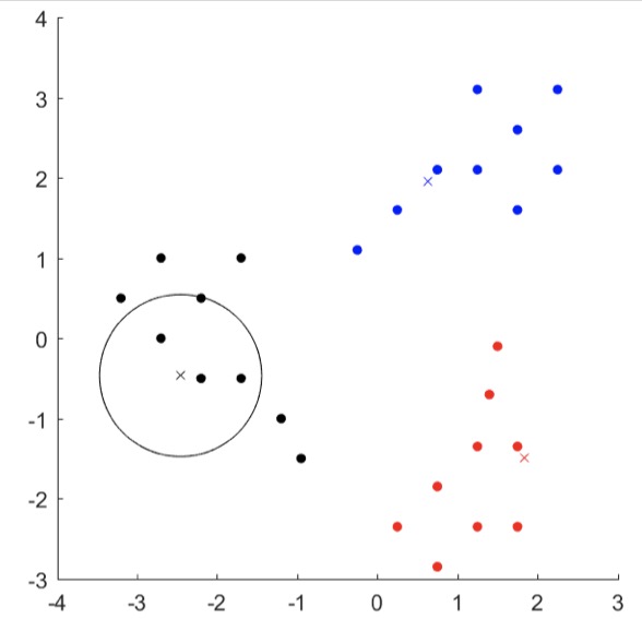
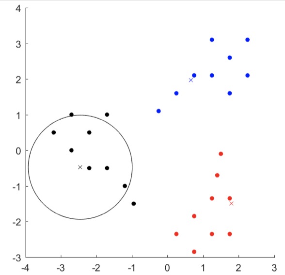
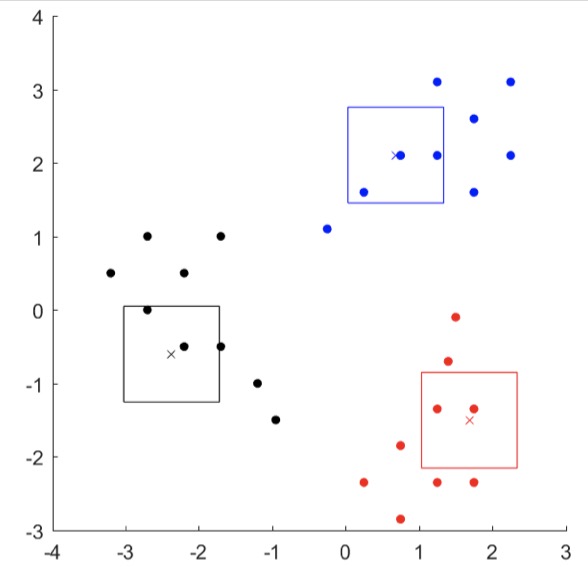
In Figures 14 – 17, all sites can be perturbed simultaneously within the drawn $p$-norm balls without changing the clustering. The different sizes of the $p$-norm balls are due to scaling of the optimal solutions of (3). Note that scaling the sites does not change the clustering, but of course, the scaling does affect the radius of the $p$-norm ball. In fact, the radius directly corresponds to the stability of the depicted optimal sites. The BHR stability of the left-hand clustering is $\tau^{2}_{\pm}(z^{(2)})\approx 0.253$ and $\tau^{\infty}_{\pm}(z^{(\infty)})\approx 0.139$, whereas for the right-hand clustering we get $\tau^{2}_{\pm}(z^{(2)})\approx 0.018$ and $\tau^{\infty}_{\pm}(z^{(\infty)})\approx 0.009$. Note that on the right-hand side of Figures 14 and 15, the balls around each cross that indicate the area of possible perturbation are so small that they become hard to see.

Figures 16 and 17 depict the areas of perturbation for the single-shape partition polytope. The difference between left-hand and right-hand clustering of the LSA stability is not as large as in the previous examples, since the cluster sizes are fixed. We obtain $\tau^{2}_{=}(z^{(2)})\approx 0.365$, $\tau^{\infty}_{=}(z^{(\infty)})\approx 0.163$ (left) and $\tau^{2}_{=}(z^{(2)})\approx 0.199$, $\tau^{\infty}_{=}(z^{(\infty)})\approx 0.100$ (right). Nevertheless, one sees that the sites on the left-hand side can be perturbed more than the ones on the right-hand side.

References

- [1] D. Aloise, A. Deshpande, P. Hansen, and P. Popat. NP-hardness of Euclidean sum-of-squares clustering. Machine Learning, 75:245–249, 2009.
- [2] E. Anderes, S. Borgwardt, and J. Miller. Discrete Wasserstein Barycenters: Optimal Transport for Discrete Data. Mathematical Methods of Operations Research, 84(2):389–409, 2016.
- [3] F. Aurenhammer. Power Diagrams: Properties, Algorithms and Applications. SIAM Journal on Computing, 16(1):78–96, 1987.
- [4] F. Aurenhammer, F. Hoffmann, and B. Aronov. Minkowski-Type Theorems and Least-Squares Clustering. Algorithmica, 20(1):61–76, 1998.
- [5] Sharon Aviran, Nissan Lev-Tov, Shmuel Onn, and Uriel G. Rothblum. Vertex Characterization of Partition Polytopes of Bipartitions and of Planar Point Sets. Discrete Applied Mathematics, 124(1):1 – 15, 2002.
- [6] M. Balinski and A. Russakoff. On the Assignment Polytope. SIAM Review, 16(4), 1974.
- [7] E. R. Barnes, A. J. Hoffman, and U. G. Rothblum. Optimal Partitions Having Disjoint Convex and Conic Hulls. Mathematical Programming, 54(1):69–86, 1992.
- [8] K. P. Bennett and O. L. Mangasarian. Multicategory discrimination via linear programming. Optimization Methods and Software, 3:27–39, 1992.
- [9] P. Berkhin. Survey of clustering data mining techniques. Technical report, Accrue Software, 2002.
- [10] N. Bonifas, M. Di Summa, F. Eisenbrand, N. Hähnle, and M. Niemeier. On Sub-determinants and the Diameter of Polyhedra. Discrete & Computational Geometry, 52(1):102–115, 2014.
- [11] S. Borgwardt. A Combinatorial Optimization Approach to Constrained Clustering. Dissertation, Technische Universität München, München, 2010.
- [12] S. Borgwardt. On Soft Power Diagrams. Journal of Mathematical Modelling and Algorithms in Operations Research, 14(2):173–196, 2015.
- [13] A. Brieden and P. Gritzmann. On Optimal Weighted Balanced Clusterings: Gravity Bodies and Power Diagrams. SIAM Journal on Discrete Mathematics, 26(2):415–434, 2012.
- [14] B. Cousins. Volume Computation of Convex Bodies, June 2015. MATLAB Function available at http://www.mathworks.com/matlabcentral/fileexchange/43596-volume-computation-of-convex-bodies, accessed July 2017.
- [15] J. A. De Loera and E. D. Kim. Combinatorics and Geometry of Transportation Polytopes: An Update. Discrete Geometry and Algebraic Combinatorics, 625:37–76, 2014.
- [16] J.-P. Doignon and M. Regenwetter. An Approval-voting Polytope for Linear Orders. Journal of Mathematical Psychology, 41(2):171–188, July 1997.
- [17] K. Fukuda, S. Onn, and V. Rosta. An Adaptive Algorithm for Vector Partitioning. Journal of Global Optimization, 25(3):305–319, 2003.
- [18] B. Gao, F. K. Hwang, W.-C. W. Li, and U. G. Rothblum. Partition Polytopes Over 1-dimensional Points. Mathematical Programming, 85(2):335–362, 1999.
- [19] J. Gill and S. Linusson. The -assignment Polytope. In Discrete Optimization, volume 6(2), pages 148–161. Elsevier Science, 2009.
- [20] E. S. Gottlieb and M. R. Rao. The Generalized Assignment Problem: Valid Inequalities and Facets. Mathematical Programming, 46(1):31–52, 1990.
- [21] M. Grötschel and Y. Wakabayashi. Facets of the Clique Partitioning Polytope. Mathematical Programming, 47(1):367–387, 1990.
- [22] R. Guralnick and D. Perkinson. Permutation Polytopes and Indecomposable Elements in Permutation Groups. Journal of Combinatorial Theory, Ser. A, 113:1243–1256, 2006.
- [23] F. Happach. Stable Clusterings and the Cones of Outer Normals. Master’s thesis, Technische Universität München, München, 2016.
- [24] F. K. Hwang, S. Onn, and U. G. Rothblum. Representations and Characterizations of Vertices of Bounded-shape Partition Polytopes. Linear Algebra and its Applications, 278(1):263 – 284, 1998.
- [25] A. K. Jain, M. N. Murty, and P. J. Flynn. Data clustering - a review. In ACM Computing Surveys, volume 31-3, pages 264–323, 1999.
- [26] A. Kalman. Newton Polytopes of Cluster Variables. Dissertation, University of California, Berkeley, Berkeley, 2014.
- [27] S. P. Lloyd. Least squares quantization in pcm. IEEE Transactions on Information Theory, 28(2):129–137, 1982.
- [28] J. B. MacQueen. Some methods of classification and analysis of multivariate observations. In Proceedings of the Fifth Berkeley Symposium on Mathematical Statistics and Probability, pages 281–297, 1967.
- [29] M. Mahajan, P. Nimbhorkar, and K. Varadarajan. The planar k-means problem is NP-hard. Theoretical Computer Science, 442:13–21, 2012.
- [30] G. L. Nemhauser and L. A. Wolsey. Integer and Combinatorial Optimization. Wiley, New York, NY, 1999.
- [31] S. Onn. Geometry, Complexity, and Combinatorics of Permutation Polytopes. Journal on Combinatorial Theory, Ser. A, 64(1):31–49, 1993.
- [32] A. Schrijver. Theory of Linear and Integer Programming. John Wiley & Sons, Inc., New York, NY, USA, 1986.
- [33] R. Suck. Geometric and Combinatorial Properties of the Polytope of Binary Choice Probabilities. Mathematical Social Sciences, 23(1):81 – 102, 1992.
- [34] R. Suck. Polytopes in Measurement and Data Analysis. Review of Lectures on Polytopes, by Günther M. Ziegler. Journal of Mathematical Psychology, 41(3):299–303, 1997.
- [35] A. Vattani. k-Means requires exponentially many iterations even in the plane. Discrete Computational Geometry, 45:596–616, 2011.
- [36] U. von Luxburg. Clustering Stability: An Overview. Foundations and Trends in Machine Learning, 2(3):235–274, 2010.
- [37] R. Xu and D. Wunsch. Survey of clustering algorithms. In IEEE Transactions on Neural Networks, volume 16:3, pages 645–678, 2005.
- [38] G. M. Ziegler. Lectures on Polytopes, volume 152 of Graduate Texts in Mathematics. Springer Verlag, 1995.