Hamilton-Jacobi equations for optimal control on networks with entry or exit costs

Manh Khang DAO ^†^†thanks: IRMAR, Université de Rennes 1, 35000 Rennes, France. manh-khang.dao@univ-rennes1.fr

August 24, 2026

Abstract

We consider an optimal control on networks in the spirit of the works of Achdou et al. (2013) and Imbert et al. (2013). The main new feature is that there are entry (or exit) costs at the edges of the network leading to a possible discontinuous value function. We characterize the value function as the unique viscosity solution of a new Hamilton-Jacobi system. The uniqueness is a consequence of a comparison principle for which we give two different proofs, one with arguments from the theory of optimal control inspired by Achdou et al. (2014) and one based on partial differential equations techniques inspired by a recent work of Lions and Souganidis (2016).

Key words: Optimal control, networks, Hamilton-Jacobi equation, viscosity solutions, uniqueness, switching cost
AMS subject classification: 34H05, 35F21, 49L25, 49J15, 49L20, 93C30

1 Introduction

A network (or a graph) is a set of items, referred to as vertices or nodes, which are connected by edges (see Figure 1 for example). Recently, several research projects have been devoted to dynamical systems and differential equations on networks, in general or more particularly in connection with problems of data transmission or traffic management (see for example Garavello and Piccoli [14] and Engel et al [12]).

An optimal control problem is an optimization problem where an agent tries to minimize a cost which depends on the solution of a controlled ordinary differential equation (ODE). The ODE is controlled in the sense that it depends on a function called the control. The goal is to find the best control in order to minimize the given cost. In many situations, the optimal value of the problem as a function of the initial state (and possibly of the initial time when the horizon of the problem is finite) is a viscosity solution of a Hamilton-Jacobi-Bellman partial differential equation (HJB equation). Under appropriate conditions, the HJB equation has a unique viscosity solution characterizing by this way the value function. Moreover, the optimal control may be recovered from the solution of the HJB equation, at least if the latter is smooth enough.

The first articles about optimal control problems in which the set of admissible states is a network (therefore the state variable is a continuous one) appeared in 2012: in [2], Achdou et al. derived the HJB equation associated to an infinite horizon optimal control on a network and proposed a suitable notion of viscosity solution. Obviously, the main difficulties arise at the vertices where the network does not have a regular differential structure. As a result, the new admissible test-functions whose restriction to each edge is $C^{1}$ are applied. Independently and at the same time, Imbert et al. [17] proposed an equivalent notion of viscosity solution for studying a Hamilton-Jacobi approach to junction problems and traffic flows. Both [2] and [17] contain first results on comparison principles which were improved later. It is also worth mentioning the work by Schieborn and Camilli [22], in which the authors focus on eikonal equations on networks and on a less general notion of viscosity solution. In the particular case of eikonal equations, Camilli and Marchi established in [10] the equivalence between the definitions given in [2, 17, 22].

Since 2012, several proofs of comparison principles for HJB equations on networks, giving uniqueness of the solution, have been proposed.

1.

In [3], Achdou et al. give a proof of a comparison principle for a stationary HJB equation arising from an optimal control with infinite horizon, (therefore the Hamiltonian is convex) by mixing arguments from the theory of optimal control and PDE techniques. Such a proof was much inspired by works of Barles et al. [7, 6], on regional optimal control problems in ${\mathbb{R}}^{d}$ , (with discontinuous dynamics and costs).
2.

A different and more general proof, using only arguments from the theory of PDEs was obtained by Imbert and Monneau in [16]. The proof works for quasi-convex Hamiltonians, and for stationary and time-dependent HJB equations. It relies on the construction of suitable vertex test functions.
3.

A very simple and elegant proof, working for non convex Hamiltonians, has been very recently given by Lions and Souganidis [19, 20].

The goal of this paper is to consider an optimal control problem on a network in which there are entry (or exit) costs at each edge of the network and to study the related HJB equations. The effect of the entry/exit costs is to make the value function of the problem discontinuous. Discontinuous solutions of Hamilton-Jacobi equation have been studied by various authors, see for example Barles [4], Frankowska and Mazzola [13], and in particular Graber et al. [15] for different HJB equations on networks with discontinuous solutions.

To simplify the problem, we will first study the case of junction, i.e., a network of the form $\mathcal{G}=\cup_{i=1}^{N}\Gamma_{i}$ with $N$ edges $\Gamma_{i}$ ( $\Gamma_{i}$ is the closed half line ${\mathbb{R}}^{+}e_{i}$ ) and only one vertex $O$ , where $\{O\}=\cap_{i=1}^{N}\Gamma_{i}$ . Later, we will generalize our analysis to networks with an arbitrary number of vertices. In the case of the junction described above, our assumptions about the dynamics and the running costs are similar to those made in [3], except that additional costs $c_{i}$ for entering the edge $\Gamma_{i}$ at $O$ or $d_{i}$ for exiting $\Gamma_{i}$ at $O$ are added in the cost functional. Accordingly, the value function is continuous on $\mathcal{G}$ , but is in general discontinuous at the vertex $O$ . Hence, instead of considering the value function $\mathsf{v}$ , we split it into the collection $(v_{i})_{1\leq i\leq N}$ , where $v_{i}$ is continuous function defined on the edge $\Gamma_{i}$ . More precisely,

v_{i}\left(x\right)=\begin{cases}\mathsf{v}\left(x\right)&\text{if }x\in\Gamma_{i}\backslash\left\{O\right\},\\ \lim_{\delta\rightarrow 0^{+}}\mathsf{v}\left(\delta e_{i}\right)&\text{if }x=O.\end{cases}

Our approach is therefore reminiscent of optimal switching problems (impulsional control): in the present case the switches can only occur at the vertex $O$ . Note that our assumptions will ensure that $\mathsf{v}|_{\Gamma_{i}\setminus\{O\}}$ is Lipschitz continuous near $O$ and that $\lim_{\delta\rightarrow 0^{+}}\mathsf{v}\left(\delta e_{i}\right)$ does exist. In the case of entry costs for example, our first main result will be to find the relation between $\mathsf{v}\left(O\right)$ , $v_{i}\left(O\right)$ and $v_{j}\left(O\right)+c_{j}$ for $i,j=\overline{1,N}$ .

This will show that the functions $(v_{i})_{1\leq i\leq N}$ are (suitably defined) viscosity solutions of the following system

\begin{array}[]{cc}\lambda u_{i}\left(x\right)+H_{i}\left(x,\dfrac{du_{i}}{dx_{i}}\left(x\right)\right)=0&\mbox{if $x\in\Gamma_{i}\backslash\left\{O\right\}$,}\\ {\displaystyle\lambda u_{i}\left(O\right)+\max\left\{-\lambda\min_{j\neq i}\left\{u_{j}\left(O\right)+c_{j}\right\},H_{i}^{+}\left(O,\dfrac{du_{i}}{dx_{i}}\left(O\right)\right),H_{O}^{T}\right\}=0}&\mbox{if $x=O$}.\end{array}

(1.1)

Here $H_{i}$ is the Hamiltonian corresponding to edge $\Gamma_{i}$ . At vertex $O$ , the definition of the Hamiltonian has to be particular, in order to consider all the possibilities when $x$ is close to $O$ . More specifically, if $x$ is close to $O$ and belongs to $\Gamma_{i}$ then:

•

The term $\min_{j\neq i}\left\{u_{j}\left(O\right)+c_{j}\right\}$ accounts for situations in which the trajectory enters $\Gamma_{i_{0}}$ where $u_{i_{0}}\left(O\right)+c_{i_{0}}=\min_{j\neq i}\left\{u_{j}\left(O\right)+c_{j}\right\}$ .
•

The term $H_{i}^{+}\left(O,\dfrac{du_{i}}{dx_{i}}\left(O\right)\right)$ accounts for situations in which the trajectory does not leave $\Gamma_{i}$ .
•

The term $H_{O}^{T}$ accounts for situations in which the trajectory stays at $O$ .

The most important part of the paper will be devoted to two different proofs of a comparison principle leading to the well-poseness of (1.1): the first one uses arguments from optimal control theory coming from Barles et al. [6, 7] and Achdou et al. [3]; the second one is inspired by Lions and Souganidis [19] and uses arguments from the theory of PDEs.

The paper is organized as follows: Section 2 deals with the optimal control problems with entry and exit costs: we give a simple example in which the value function is discontinuous at the vertex $O$ , and also prove results on the structure of the value function near $O$ . In Section 3, the new system of (1.1) is defined and a suitable notion of viscosity solutions is proposed. In Section 4, we prove our value functions are viscosity solutions of the above mentioned system. In Section 5, some properties of viscosity sub and super-solution are given and used to obtain the comparison principle. Finally, optimal control problems with entry costs which may be zero and related HJB equations are considered in Section 6.

Refer to caption — Figure 1: The network $\mathcal{G}$ ( $N=5$ )

2 Optimal control problem on junction with entry/exit costs

2.1 The geometry

We consider the model case of the junction in $\mathbb{R}^{d}$ with $N$ semi-infinite straight edges, $N>1$ . The edges are denoted by $\left(\Gamma_{i}\right)_{i=\overline{1,N}}$ where $\Gamma_{i}$ is the closed half-line $\mathbb{R}^{+}e_{i}$ . The vectors $e_{i}$ are two by two distinct unit vectors in $\mathbb{R}^{d}$ . The half-lines $\Gamma_{i}$ are glued at the vertex $O$ to form the junction $\mathcal{G}$

\mathcal{G}=\bigcup_{i=1}^{N}\Gamma_{i}.

The geodetic distance $d\left(x,y\right)$ between two points $x,y$ of $\mathcal{G}$ is

d\left(x,y\right)=\begin{cases}\left|x-y\right|&\mbox{if }x,y\mbox{ belong to the same egde }\Gamma_{i},\\ \left|x\right|+\left|y\right|&\mbox{if }x,y\mbox{ belong to different edges }\Gamma_{i}\mbox{ and }\Gamma_{j}.\end{cases}

2.2 The optimal control problem

We consider infinite horizon optimal control problems which have different dynamic and running costs for each and every edge. For $i=\overline{1,N}$ ,

•

the set of control on $\Gamma_{i}$ is denoted by $A_{i}$
•

the system is driven by a dynamics $f_{i}$
•

there is a running cost $\ell_{i}$ .

Our main assumptions, referred to as $\left[H\right]$ hereafter, are as follows:

$\left[H0\right]$ (Control sets) Let $A$ be a metric space (one can take $A=\mathbb{R}^{d}$ . For $i=\overline{1,N}$ , $A_{i}$ is a nonempty compact subset of $A$ and the sets $A_{i}$ are disjoint.

$\left[H1\right]$ (Dynamics) For $i=\overline{1,N}$ , the function $f_{i}:\Gamma_{i}\times A_{i}\rightarrow\mathbb{R}$ is continuous and bounded by $M$ . Moreover, there exists $L>0$ such that

\left|f_{i}\left(x,a\right)-f_{i}\left(y,a\right)\right|\leq L\left|x-y\right|\quad\mbox{ for all }x,y\in\Gamma_{i},a\in A_{i}.

Hereafter, we will use the notation $F_{i}\left(x\right)$ for the set $\left\{f_{i}\left(x,a\right)e_{i}:a\in A_{i}\right\}$ .

$\left[H2\right]$ (Running costs) For $i=\overline{1,N}$ , the function $\ell_{i}:\Gamma_{i}\times A_{i}\rightarrow\mathbb{R}$ is a continuous function bounded by $M>0$ . There exists a modulus of continuity $\omega$ such that

\left|\ell_{i}\left(x,a\right)-\ell_{i}\left(y,a\right)\right|\leq\omega\left(\left|x-y\right|\right)\quad\mbox{ for all }x,y\in\Gamma_{i},a\in A_{i}.

$\left[H3\right]$ (Convexity of dynamic and costs) For $x\in\Gamma_{i}$ , the following set

\mbox{FL}_{i}\left(x\right)=\left\{\left(f_{i}\left(x,a\right)e_{i},\ell_{i}\left(x,a\right)\right):a\in A_{i}\right\}

is non-empty, closed and convex.

$\left[H4\right]$ (Strong controllability) There exists a real number $\delta>0$ such that

\left[-\delta e_{i},\delta e_{i}\right]\subset F_{i}\left(O\right)=\left\{f_{i}\left(O,a\right)e_{i}:a\in A_{i}\right\}.

Remark 2.1.

The assumption that the sets $A_{i}$ are disjoint is not restrictive. Indeed, if $A_{i}$ are not disjoint, then we define $\tilde{A}_{i}=A_{i}\times\left\{i\right\}$ and $\tilde{f}_{i}\left(x,\tilde{a}\right)=f_{i}\left(x,a\right),\tilde{\ell}_{i}\left(x,\tilde{a}\right)=\ell_{i}\left(x,a\right)$ with $\tilde{a}=\left(a,i\right)$ with $a\in A_{i}$ . The assumption $\left[H3\right]$ is made to avoid the use of relaxed control. With assumption $\left[H4\right]$ , one gets that the Hamiltonian which will appear later is coercive for $x$ close to the $O$ . Moreover, $\left[H4\right]$ is an important assumption to prove Lemma 2.7 and Lemma 5.3.

Let

\mathcal{M}=\left\{\left(x,a\right):x\in\mathcal{G},a\in A_{i}\mbox{ if }x\in\Gamma_{i}\backslash\left\{O\right\},\mbox{ and }a\in\cup_{i=1}^{N}A_{i}\mbox{ if }x=O\right\}.

Then $\mathcal{M}$ is closed. We also define the function on $\mathcal{M}$ by

\mbox{for all}\left(x,a\right)\in\mathcal{M},\quad f\left(x,a\right)=\begin{cases}f_{i}\left(x,a\right)e_{i}&\quad\mbox{if }x\in\Gamma_{i}\backslash\left\{O\right\}\mbox{ and }a\in A_{i},\\ f_{i}\left(O,a\right)e_{i}&\quad\mbox{if }x=O\mbox{ and }a\in A_{i}.\end{cases}

The function $f$ is continuous on $\mathcal{M}$ since the sets $A_{i}$ are disjoint.

Definition 2.2 (The speed set and the admissible control set).

The set $\tilde{F}\left(x\right)$ which contains all the “possible speeds” at $x$ is defined by

\tilde{F}\left(x\right)=\begin{cases}F_{i}\left(x\right)&\quad\mbox{if }x\in\Gamma_{i}\backslash\left(O\right),\\ \bigcup_{i=1}^{N}F_{i}\left(O\right)&\quad\mbox{if $x=O$}.\end{cases}

For $x\in\mathcal{G}$ , the set of admissible trajectories starting from $x$ is

Y_{x}=\left\{y_{x}\in Lip\left(\mathbb{R}^{+};\mathcal{G}\right):\begin{cases}\dot{y}_{x}\left(t\right)&\in\tilde{F}\left(y_{x}\left(t\right)\right)\quad\mbox{for a.e. }t>0\\ y_{x}\left(0\right)&=x\end{cases}\right\}.

According to [3, Theorem 1.2], a solution $y_{x}$ can be associated with several control laws. We introduce the set of admissible controlled trajectories starting from $x$

\mathcal{T}_{x}=\left\{\left(y_{x},\alpha\right)\in L_{loc}^{\infty}\left(\mathbb{R}^{+};\mathcal{M}\right):y_{x}\in Lip\left(\mathbb{R}^{+};\mathcal{G}\right)\mbox{ and }y_{x}\left(t\right)=x+\int_{0}^{t}f\left(y_{x}\left(s\right),\alpha\left(s\right)\right)ds\right\}.

Notice that, if $\left(y_{x},\alpha\right)\in\mathcal{T}_{x}$ then $y_{x}\in Y_{x}$ . Hereafter, we will denote $y_{x}$ by $y_{x,\alpha}$ if $\left(y_{x},\alpha\right)\in\mathcal{T}_{x}$ . For any $y_{x,\alpha}$ , we can define the closed set $T_{O}=\left\{t\in\mathbb{R}^{+}:y_{x,\alpha}\left(t\right)=O\right\}$ and the open set $T_{i}$ in $\mathbb{R}^{+}=\left[0,+\infty\right)$ by $T_{i}=\left\{t\in\mathbb{R}^{+}:y_{x,\alpha}\left(t\right)\in\Gamma_{i}\backslash\left\{O\right\}\right\}$ . The set $T_{i}$ is a countable union of disjoint open intervals

T_{i}=\bigcup_{k\in K_{i}\subset\mathbb{N}}T_{ik}=\begin{cases}\left[0,\eta_{i0}\right)\cup\bigcup_{k\in K_{i}\subset\mathbb{N^{\star}}}\left(t_{ik},\eta_{ik}\right)&\quad\mbox{if }x\in\Gamma_{i}\backslash\left\{O\right\},\\ \bigcup_{k\in K_{i}\subset\mathbb{N^{\star}}}\left(t_{ik},\eta_{ik}\right)&\quad\mbox{if }x\notin\Gamma_{i}\backslash\left\{O\right\},\end{cases}

where $K_{i}=\overline{1,n}$ if the trajectory $y_{x,\alpha}$ enters $\Gamma_{i}$ $n$ times and $K_{i}=\mathbb{N}$ if the trajectory $y_{x,\alpha}$ enters $\Gamma_{i}$ infinite times.

Remark 2.3.

From the above definition, one can see that $t_{ik}$ is an entry time in $\Gamma_{i}\backslash\left\{O\right\}$ and $\eta_{ik}$ is an exit time from $\Gamma_{i}\backslash\left\{O\right\}$ . Hence

y_{x,\alpha}\left(t_{ik}\right)=y_{x,\alpha}\left(\eta_{ik}\right)=O.

Let $C=\left\{c_{1},c_{2},\ldots,c_{N}\right\}$ be a set of entry costs and $D=\left\{d_{1},d_{2},\ldots,d{}_{N}\right\}$ be a set of exit costs. We underline that, except in Section 6, entry and exist costs are positive.

In the sequel, we define two different cost functionals (the first one corresponds to the case when there is a cost for entering the edges and the second one corresponds to the case when there is a cost for exiting the edges):

Definition 2.4 (The cost functionals and value functions with entry/exit costs).

The costs associated to trajectory $\left(y_{x,\alpha},\alpha\right)\in\mathcal{T}_{x}$ are defined by

J\left(x;\left(y_{x,\alpha},\alpha\right)\right)=\int_{0}^{+\infty}\ell\left(y_{x,\alpha}\left(t\right),\alpha\left(t\right)\right)e^{-\lambda t}dt+\sum_{i=1}^{N}\sum_{k\in K_{i}}c_{i}e^{-\lambda t_{ik}}\quad\mbox{(cost functional with entry cost)},

and

\widehat{J}\left(x;\left(y_{x,\alpha},\alpha\right)\right)=\int_{0}^{+\infty}\ell\left(y_{x,\alpha}\left(t\right),\alpha\left(t\right)\right)e^{-\lambda t}dt+\sum_{i=1}^{N}\sum_{k\in K_{i}}d_{i}e^{-\lambda\eta_{ik}}\quad\mbox{(cost functional with exit cost)},

where the running cost $\ell:\mathcal{M}\rightarrow\mathbb{R}$ is

\ell\left(x,a\right)=\begin{cases}\ell_{i}\left(x,a\right)&\quad\mbox{if $x\in\Gamma_{i}\backslash\left\{O\right\}$}\mbox{ and }a\in A_{i},\\ \ell_{i}\left(O,a\right)&\quad\mbox{if }x=0\mbox{ and }a\in A_{i}.\end{cases}

Hereafter, to simplify the notation, we will use $J\left(x,\alpha\right)$ and $\widehat{J}\left(x,\alpha\right)$ instead of $J\left(x;\left(y_{x,\alpha},\alpha\right)\right)$ and $\widehat{J}\left(x;\left(y_{x,\alpha},\alpha\right)\right)$ , respectively.

The value functions of the infinite horizon optimal control problem are defined by:

\mathsf{v}\left(x\right)=\inf_{\left(y_{x,\alpha},\alpha\right)\in\mathcal{T}_{x}}J\left(x;\left(y_{x,\alpha},\alpha\right)\right)\quad\mbox{(value function with entry cost)},

and

\widehat{\mathsf{v}}\left(x\right)=\inf_{\left(y_{x,\alpha},\alpha\right)\in\mathcal{T}_{x}}\widehat{J}\left(x;\left(y_{x,\alpha},\alpha\right)\right)\quad\mbox{(value function with exit cost)}.

Remark 2.5.

By the definition of the value function, we are mainly interested in a control law $\alpha$ such that $J\left(x,\alpha\right)<+\infty$ . In such a case, if $\left|K_{i}\right|=+\infty$ , then we can order $\left\{t_{ik},\eta_{ik}:\;k\in\mathbb{N}\right\}$ such that

t_{i1}<\eta_{i1}<t_{i2}<\eta_{i2}<\ldots<t_{ik}<\eta_{ik}<\ldots,

and

\lim_{k\rightarrow\infty}t_{ik}=\lim_{k\rightarrow\infty}\eta_{ik}=+\infty.

Indeed, assuming if $\lim_{k\rightarrow\infty}t_{ik}=\overline{t}<+\infty$ , then

\displaystyle J\left(x,\alpha\right)

\displaystyle\geq

\displaystyle-\dfrac{M}{\lambda}+\sum_{k=1}^{+\infty}e^{-\lambda t_{ik}}c_{i}=-\dfrac{M}{\lambda}+c_{i}\sum_{k=1}^{+\infty}e^{-\lambda t_{ik}}=+\infty,

in contradiction with $J\left(x,\alpha\right)<+\infty$ . This means that the state cannot switch edges infinitely many times in finite time, otherwise the cost functional is obviously infinite.

The following example shows that the value function with entry costs is possibly discontinuous (The same holds for the value function with exit costs).

Example 2.6.

Consider the network $\mathcal{G}=\Gamma_{1}\cup\Gamma_{2}$ where $\Gamma_{1}=\mathbb{R}^{+}e_{1}=\left(-\infty,0\right]$ and $\Gamma_{2}=\mathbb{R}^{+}e_{2}=\left[0,+\infty\right)$ . The control sets are $A_{i}=\left[-1,1\right]\times\left\{i\right\}$ with $i\in\left\{1,2\right\}$ . Set

\left(f\left(x,a\right),\ell\left(x,a\right)\right)=\begin{cases}\left(f_{i}\left(x,\left(a_{i},i\right)\right)e_{i},\ell_{i}\left(x,\left(a_{i},i\right)\right)\right)&\text{if }x\in\Gamma_{i}\backslash\left\{O\right\}\text{ and }a=\left(a_{i},i\right)\in A_{i},\\ \left(f_{i}\left(O,\left(a_{i},i\right)\right)e_{i},\ell_{i}\left(O,\left(a_{i},i\right)\right)\right)&\text{if }x=O\text{ and }a=\left(a_{i},i\right)\in A_{i},\end{cases}

where $f_{i}\left(x,\left(a_{i},i\right)\right)=a_{i}$ and $\ell_{1}\equiv 1,\ell_{2}\left(x,\left(a_{2},2\right)\right)=1-a_{2}$ . For $x\in\Gamma_{2}\backslash\left\{O\right\}$ , then $\mathsf{v}\left(x\right)=v_{2}\left(x\right)=0$ with optimal strategy consists in choosing $\alpha\left(t\right)\equiv\left(1,2\right)$ . For $x\in\Gamma_{1}$ , we can check that $\mathsf{v}\left(x\right)=\min\left\{\dfrac{1}{\lambda},\dfrac{1-e^{-\lambda\left|x\right|}}{\lambda}+c_{2}e^{-\lambda\left|x\right|}\right\}$ . More precisely, for all $x\in\Gamma_{1}$ , we have

\mathsf{v}\left(x\right)=\begin{cases}\dfrac{1}{\lambda}&\text{if }c_{2}\geq\dfrac{1}{\lambda},\text{ with the optimal control $\alpha\left(t\right)\equiv\left(-1,1\right)$},\\ \dfrac{1-e^{-\lambda\left|x\right|}}{\lambda}+c_{2}e^{-\lambda\left|x\right|}&\text{if }c_{2}<\dfrac{1}{\lambda},\text{ with the optimal control $\alpha\left(t\right)=\begin{cases}\left(1,1\right)&\text{if }t\leq\left|x\right|,\\ \left(1,2\right)&\text{if }t\geq\left|x\right|.\end{cases}$}\end{cases}

Summarizing, we have the two following cases

If $c_{2}\geq\dfrac{1}{\lambda}$ , then

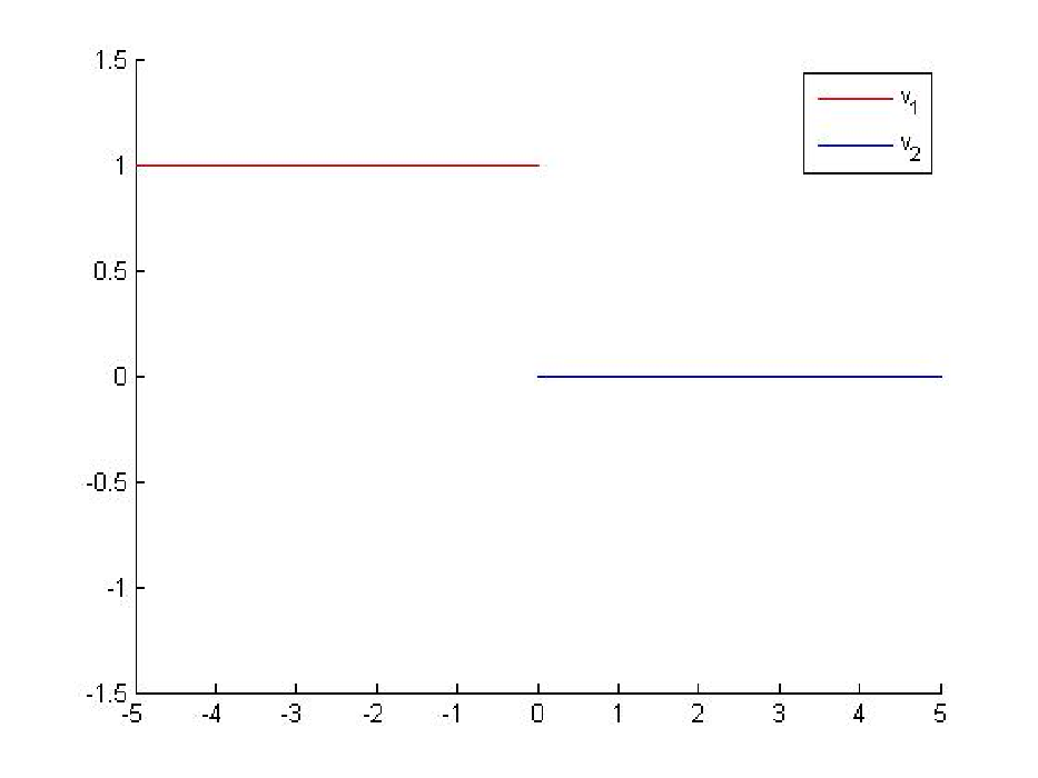
\mathsf{v}\left(x\right)=\begin{cases}0&\quad\mbox{if }x\in\Gamma_{2}\backslash\left\{O\right\},\\ \dfrac{1}{\lambda}&\quad\mbox{if }x\in\Gamma_{1}.\end{cases}

The graph of the value function with entry costs $c_{2}\geq\dfrac{1}{\lambda}=1$ is plotted in Figure 2a.

If $c_{2}<\dfrac{1}{\lambda}$ , then

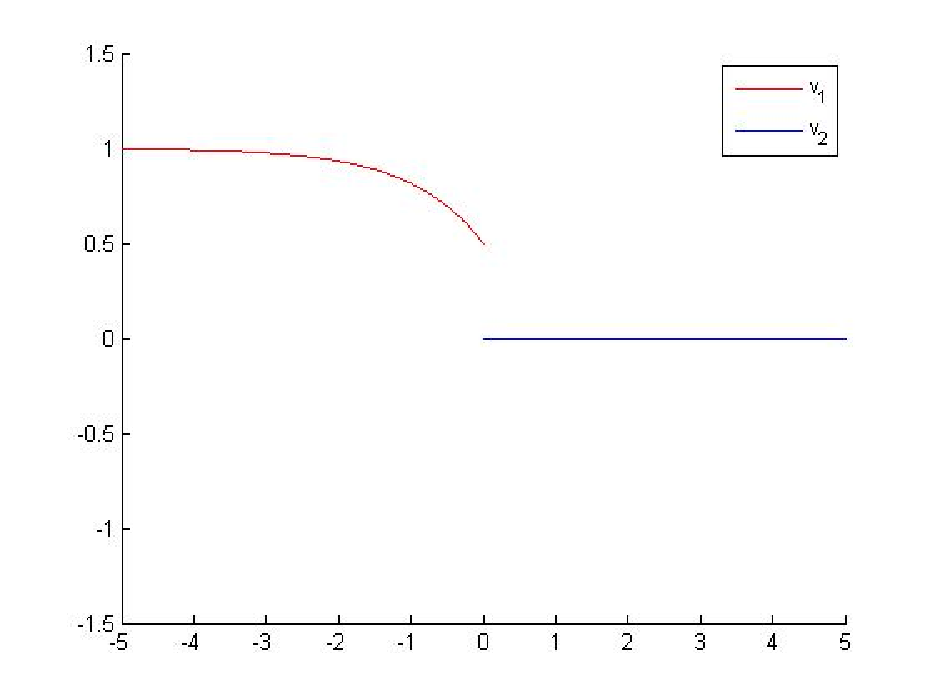
\mathsf{v}\left(x\right)=\begin{cases}0&\quad\mbox{if }x\in\Gamma_{2}\backslash\left\{O\right\},\\ \dfrac{1-e^{-\lambda\left|x\right|}}{\lambda}+c_{2}e^{-\lambda\left|x\right|}&\quad\mbox{if }x\in\Gamma_{1}.\end{cases}

The graph of the value function with entry costs $c_{2}=\dfrac{1}{2}<1=\dfrac{1}{\lambda}$ is plotted in Figure 2b.

Lemma 2.7.

Under assumptions $\left[H1\right]$ and $\left[H4\right]$ , there exist two positive numbers $r_{0}$ and $C$ such that for all $x_{1},x_{2}\in B\left(O,r_{0}\right)\cap\mathcal{G}$ , there exists $\left(y_{x_{1},\alpha_{x_{1},x_{2}}},\alpha_{x_{1},x_{2}}\right)\in\mathcal{T}_{x_{1}}$ and $\tau_{x_{1},x_{2}}\leq Cd\left(x_{1},x_{2}\right)$ such that $y_{x_{1}}\left(\tau_{x_{1},x_{2}}\right)=x_{2}$ .

Proof of Lemma 2.7.

This proof is classical. It is sufficient to consider the case when $x_{1}$ and $x_{2}$ belong to same edge $\Gamma_{i}$ , since in the other cases, we will use $O$ as a connecting point between $x_{1}$ and $x_{2}$ . According to Assumption $\left[H4\right]$ , there exists $a\in A_{i}$ such that $f_{i}\left(O,a\right)=\delta$ . Additionally, by the Lipschitz continuity of $f_{i}$ ,

\left|f_{i}\left(O,a\right)-f_{i}\left(x,a\right)\right|\leq L\left|x\right|,

hence, if we choose $r_{0}:=\dfrac{\delta}{2L}>0$ , then $f_{i}\left(x,a\right)\geq\dfrac{\delta}{2}$ for all $x\in B\left(O,r_{0}\right)\cap\Gamma_{i}$ . Let $x_{1},x_{2}$ be in $B\left(O,r_{0}\right)\cap\Gamma_{i}$ with $\left|x_{1}\right|<\left|x_{2}\right|$ : there exist a control law $\alpha$ and $\tau_{x_{1},x_{2}}>0$ such that $\alpha\left(t\right)=a$ if $0\leq t\leq\tau_{x_{1},x_{2}}$ and $y_{x_{1},\alpha}\left(\tau_{x_{1},x_{2}}\right)=x_{2}$ . Moreover, since the velocity $f_{i}\left(y_{x_{1},\alpha}\left(t\right),\alpha\left(t\right)\right)$ is always greater than $\dfrac{\delta}{2}$ when $t\leq\tau_{x_{1},x_{2}}$ , then $\tau_{x_{1},x_{2}}\leq\dfrac{2}{\delta}d\left(x_{1},x_{2}\right).$ If $\left|x_{1}\right|>\left|x_{2}\right|$ , the proof is achieved by replacing $a\in A_{i}$ by $\overline{a}\in A_{i}$ such that $f_{i}\left(O,\overline{a}\right)=-\delta$ and applying the same argument as above. ∎

2.3 Some properties of value function at the vertex

Lemma 2.8.

Under assumption $\left[H\right]$ , $\mathsf{v}|_{\Gamma_{i}\backslash\left\{O\right\}}$ and $\widehat{\mathsf{v}}|_{\Gamma_{i}\backslash\left\{O\right\}}$ are continuous for any $i=\overline{1,N}$ . Moreover, there exists $\varepsilon>0$ such that $\mathsf{v}|_{\Gamma_{i}\backslash\left\{O\right\}}$ and $\widehat{\mathsf{v}}|_{\Gamma_{i}\backslash\left\{O\right\}}$ are Lipschitz continuous in $\left(\Gamma_{i}\backslash\left\{O\right\}\right)\cap B\left(O,\varepsilon\right)$ . Hence, it is possible to extend $\mathsf{v}|_{\Gamma_{i}\backslash\left\{O\right\}}$ and $\widehat{\mathsf{v}}|_{\Gamma_{i}\backslash\left\{O\right\}}$ at $O$ into Lipschitz continuous functions in $\Gamma_{i}\cap B\left(O,\varepsilon\right)$ . Hereafter, $v_{i}$ and $\widehat{v}_{i}$ denote these extensions.

Proof of Lemma 2.8.

The proof of continuity inside the edge is classical by using $\left[H4\right]$ , see [1] for more details. The proof of Lipschitz continuity is a consequence of Lemma 2.7. Indeed, for $x,y$ belong to $\Gamma_{i}\cap B\left(0,\varepsilon\right)$ , by Lemma 2.7 and the definition of value function, we have

\mathsf{v}\left(x\right)-\mathsf{v}\left(z\right)=v_{i}\left(x\right)-v_{i}\left(z\right)\leq\int_{0}^{\tau_{x,z}}\ell_{i}\left(y_{x,\alpha_{x,z}}\left(t\right),\alpha_{x,z}\left(t\right)\right)e^{-\lambda t}dt+v_{i}\left(z\right)\left(e^{-\lambda\tau_{x,z}}-1\right).

Since $\ell_{i}$ is bounded by $M$ (by $\left[H2\right]$ ), $v_{i}$ is bounded in $\Gamma_{i}\cap B\left(O,\varepsilon\right)$ and $e^{-\lambda\tau_{x,z}}-1$ is bounded by $\tau_{x,y}$ , there exists a constant $\overline{C}$ such that

v_{i}\left(x\right)-v_{i}\left(z\right)\leq\overline{C}\tau_{x,z}\leq\overline{C}C\left|x-z\right|.

The last inequality follows from the Lemma 2.7. The inequality $v_{i}\left(z\right)-v_{i}\left(x\right)\leq\overline{C}C\left|x-z\right|$ is obtained in a similar way. The proof is done. ∎

Let us define the tangential Hamiltonian $H_{O}^{T}$ at vertex $O$ by

H_{O}^{T}={\displaystyle\max_{i=\overline{1,N}}\max_{a_{i}\in A_{i}^{O}}\left\{-\ell_{j}\left(O,a_{j}\right)\right\}}={\displaystyle-\min_{i=\overline{1,N}}\min_{a_{i}\in A_{i}^{O}}\left\{\ell_{j}\left(O,a_{j}\right)\right\}},

(2.1)

where $A_{i}^{O}=\left\{a_{i}\in A_{i}:f_{i}\left(O,a_{i}\right)=0\right\}.$ The relationship between the values $\mathsf{v}(O)$ , $v_{i}\left(O\right)$ and $H_{O}^{T}$ will be given in the next theorem. Hereafter, the proofs of the results will be supplied only for the value function with entry costs $\mathsf{v}$ , the proofs concerning the value function with exit costs $\widehat{\mathsf{v}}$ are totally similar.

Theorem 2.9.

Under assumption $\left[H\right]$ , the value functions $\mathsf{v}$ and $\widehat{\mathsf{v}}$ satisfy

\mathsf{v}\left(O\right)=\min\left\{\min_{i=\overline{1,N}}\left\{v_{i}\left(O\right)+c_{i}\right\},-\dfrac{H_{O}^{T}}{\lambda}\right\},

and

\widehat{\mathsf{v}}\left(O\right)=\min\left\{\min_{i=\overline{1,N}}\left\{\widehat{v}_{i}\left(O\right)\right\},-\dfrac{H_{O}^{T}}{\lambda}\right\}.

Remark 2.10.

Theorem 2.9 gives us the characterization of the value function at vertex $O$ .

The proof of Theorem 2.9, makes use of Lemma 2.11 and Lemma 2.12 below.

Lemma 2.11 (Value functions $\mathsf{v}$ and $\widehat{\mathsf{v}}$ at $O$ ).

Under assumption $\left[H\right]$ , then

\max_{i=\overline{1,N}}\left\{v_{i}\left(O\right)\right\}\leq\mathsf{v}\left(O\right)\leq\min_{i=\overline{1,N}}\left\{v_{i}\left(O\right)+c_{i}\right\},

and

\max_{i=\overline{1,N}}\left\{\widehat{v}_{i}\left(O\right)-d_{i}\right\}\leq\widehat{\mathsf{v}}\left(O\right)\leq\min_{i=\overline{1,N}}\left\{\widehat{v}_{i}\left(O\right)\right\}.

Proof of Lemma 2.11.

We divide the proof into two parts.

Prove that $\max_{i=\overline{1,N}}\left\{v_{i}\left(O\right)\right\}\leq\mathsf{v}\left(O\right)$ . First, we fix $i\in\left\{1,\ldots,N\right\}$ and any control law $\overline{\alpha}$ such that $\left(y_{O,\bar{\alpha}},\bar{\alpha}\right)\in\mathcal{T}_{O}$ . Let $x\in\Gamma_{i}\backslash\left\{O\right\}$ such that $\left|x\right|$ is small. From Lemma 2.7, there exists a control law $\alpha_{x,O}$ connecting $x$ and $O$ and we consider

\alpha\left(s\right)=\begin{cases}\alpha_{x,O}\left(s\right)&\quad\mbox{if }s\leq\tau_{x,O},\\ \bar{\alpha}\left(s-\tau_{x,O}\right)&\quad\mbox{if }s>\tau_{x,O}.\end{cases}

It means that the trajectory goes from $x$ to $O$ with the control law $\alpha_{x,O}$ and then proceeds with the control law $\bar{\alpha}$ . Therefore

\displaystyle\mathsf{v}\left(x\right)

\displaystyle=v_{i}\left(x\right)\leq J\left(x,\alpha\right)=\int_{0}^{\tau_{x,O}}\ell_{i}\left(y_{x,\alpha}\left(s\right)\right)e^{-\lambda s}ds+e^{-\lambda\tau_{x,O}}J\left(O,\bar{\alpha}\right).

Since $\overline{\alpha}$ is chosen arbitrarily and $\ell_{i}$ is bounded by $M$ , we get

v_{i}\left(x\right)\leq M\tau_{x,O}+e^{-\lambda\tau_{x,O}}\mathsf{v}\left(O\right).

Let $x$ tend to $O$ then $\tau_{x,O}$ tend to $0$ from Lemma 2.7. Therefore, $v_{i}\left(O\right)\leq\mathsf{v}\left(O\right)$ . Since the above inequality holds for $i=\overline{1,N}$ , we obtain that

\max_{i=\overline{1,N}}\left\{v_{i}\left(O\right)\right\}\leq\mathsf{v}\left(O\right).

Prove that $\mathsf{v}\left(O\right)\leq\min_{i=\overline{1,N}}\left\{v_{i}\left(O\right)+c_{i}\right\}$ . For $i=\overline{1,N}$ ; we claim that $\mathsf{v}\left(O\right)\leq v_{i}\left(O\right)+c_{i}$ . Consider $x\in\Gamma_{i}\backslash\left\{O\right\}$ with $\left|x\right|$ small enough and any control law $\bar{\alpha}_{x}$ such that $\left(y_{x,\bar{\alpha}_{x}},\bar{\alpha}_{x}\right)\in\mathcal{T}_{x}$ . From Lemma 2.7, there exists a control law $\alpha_{O,x}$ connecting $O$ and $x$ and we consider

\alpha\left(s\right)=\begin{cases}\alpha_{O,x}\left(s\right)&\quad\mbox{if }s\leq\tau_{O,x},\\ \bar{\alpha}_{x}\left(s-\tau_{O,x}\right)&\quad\mbox{if }s>\tau_{O,x}.\end{cases}

It means that the trajectory goes from $O$ to $x$ using the control law $\alpha_{O,x}$ then proceeds with the control law $\bar{\alpha}_{x}$ . Therefore

\mathsf{v}\left(O\right)\leq J\left(O,\alpha\right)=c_{i}+\int_{0}^{\tau_{O,x}}\ell_{i}\left(y_{O,\alpha}\left(s\right)\right)e^{-\lambda s}ds+e^{-\lambda\tau_{O,x}}J\left(x,\bar{\alpha}_{x}\right).

Since $\overline{\alpha}_{x}$ is chosen arbitrarily and $\ell_{i}$ is bounded by $M$ , we get

\mathsf{v}\left(O\right)\leq c_{i}+M\tau_{O,x}+e^{-\lambda\tau_{O,x}}v_{i}\left(x\right)

Let $x$ tend to $O$ then $\tau_{O,x}$ tends to $0$ from Lemma 2.7, then $\mathsf{v}\left(O\right)\leq c_{i}+v_{i}\left(O\right).$ Since the above inequality holds for $i=\overline{1,N}$ , we obtain that

\mathsf{v}\left(O\right)\leq\min_{i=\overline{1,N}}\left\{v_{i}\left(O\right)+c_{i}\right\}.

∎

Lemma 2.12.

The value functions $\mathsf{v}$ and $\widehat{\mathsf{v}}$ satisfy

\mathsf{v}\left(O\right),\widehat{\mathsf{v}}\left(O\right)\leq-\dfrac{H_{O}^{T}}{\lambda}

(2.2)

where $H_{O}^{T}$ is defined in (2.1).

Proof of Lemma 2.12.

From (2.1), there exists $j\in\left\{1,\ldots,N\right\}$ and $a_{j}\in A_{j}^{O}$ such that

H_{O}^{T}=-\min_{i=\overline{1,N}}\min_{a_{i}\in A_{i}^{O}}\left\{\ell_{i}\left(O,a_{i}\right)\right\}=-\ell_{j}\left(O,a_{j}\right)

Let the control law $\alpha$ be defined by $\alpha\left(s\right)\equiv a_{j}$ for all $s$ , then

\mathsf{v}\left(O\right)\leq J\left(O,\alpha\right)=\int_{0}^{+\infty}\ell_{j}\left(O,a_{j}\right)e^{-\lambda s}ds=\dfrac{\ell_{j}\left(O,a_{j}\right)}{\lambda}=-\dfrac{H_{O}^{T}}{\lambda}.

∎

We are ready to prove Theorem 2.9.

Proof of Theorem 2.9.

According to Lemma 2.11 and Lemma 2.12,

\mathsf{v}\left(O\right)\leq\min\left\{\min_{i=\overline{1,N}}\left\{v_{i}\left(O\right)+c_{i}\right\},-\dfrac{H_{O}^{T}}{\lambda}\right\}.

Assuming that

\mathsf{v}\left(O\right)<\min_{i=\overline{1,N}}\left\{v_{i}\left(O\right)+c_{i}\right\},

(2.3)

it is sufficient to prove that $\mathsf{v}\left(O\right)=-\dfrac{H_{O}^{T}}{\lambda}$ . By (2.3), there exists a sequence $\left\{\varepsilon_{n}\right\}_{n\in\mathbb{N}}$ such that $\varepsilon_{n}\rightarrow 0$ and

\mathsf{v}\left(O\right)+\varepsilon_{n}<\min_{i=\overline{1,N}}\left\{v_{i}\left(O\right)+c_{i}\right\}\quad\mbox{for all }n\in\mathbb{N}.

On the other hand, there exists an $\varepsilon_{n}$ -optimal control $\alpha_{n}$ , $\mathsf{v}\left(O\right)+\varepsilon_{n}>J\left(O,\alpha_{n}\right)$ . Let us define the first time that the trajectory $y_{O,\alpha_{n}}$ leaves $O$

t_{n}:=\inf_{i=\overline{1,N}}T_{i}^{n},

where $T_{i}^{n}$ is the set of times $t$ for which $y_{O,\alpha_{n}}(t)$ belongs to $\Gamma_{i}\backslash\left\{O\right\}$ . Notice that $t_{n}$ is possibly $+\infty$ , in which case $y_{O,\alpha_{n}}\left(s\right)=O$ for all $s\in\left[0,+\infty\right)$ . Extracting a subsequence if necessary, we may assume that $t_{n}$ tends to $\overline{t}\in\left[0,+\infty\right]$ when $\varepsilon_{n}$ tends to $0$ .

If there exists a subsequence of $\left\{t_{n}\right\}_{n\in\mathbb{N}}$ (which is still noted $\left\{t_{n}\right\}_{n\in\mathbb{N}}$ ) such that $t_{n}=+\infty$ for all $n\in\mathbb{N}$ , then for a.e. $s\in\left[0,+\infty\right)$

\begin{cases}f\left(y_{O,\alpha_{n}}\left(s\right),\alpha_{n}\left(s\right)\right)&=f\left(O,\alpha_{n}\left(s\right)\right)=0,\\ \ell\left(y_{O,\alpha_{n}}\left(s\right),\alpha_{n}\left(s\right)\right)&=\ell\left(O,\alpha_{n}\left(s\right)\right).\end{cases}

In this case, $\alpha_{n}\left(s\right)\in\cup_{i=1}^{N}A_{i}^{O}$ for a.e. $s\in\left[0,+\infty\right)$ . Therefore, for a.e. $s\in\left[0,+\infty\right)$

\ell\left(y_{O,\alpha_{n}}\left(s\right),\alpha_{n}\left(s\right)\right)=\ell\left(O,\alpha_{n}\left(s\right)\right)\geq-H_{O}^{T},

and

\mathsf{v}\left(O\right)+\varepsilon_{n}>J\left(O,\alpha_{n}\right)=\int_{0}^{+\infty}\ell\left(O,\alpha_{n}\left(s\right)\right)e^{-\lambda s}ds\geq\int_{0}^{+\infty}\left(-H_{O}^{T}\right)e^{-\lambda s}ds=-\dfrac{H_{O}^{T}}{\lambda}.

By letting $n$ tend to $\infty$ , we get $\mathsf{v}\left(O\right)\geq-\dfrac{H_{O}^{T}}{\lambda}$ . On the other hand, since $\mathsf{v}\left(O\right)\leq-\dfrac{H_{O}^{T}}{\lambda}$ by Lemma 2.12, this implies that $\mathsf{v}\left(O\right)=-\dfrac{H_{O}^{T}}{\lambda}$ .

Let us now assume that $0\leq t_{n}<+\infty$ for all $n$ large enough. Then, for a fixed $n$ and for any positive $\delta\leq\delta_{n}$ where $\delta_{n}$ small enough, $y_{O,\alpha_{n}}\left(s\right)$ still belongs to some $\Gamma_{i\left(n\right)}\backslash\left\{O\right\}$ for all $s\in\left(t_{n},t_{n}+\delta\right]$ . We have

$\displaystyle\mathsf{v}\left(O\right)+\varepsilon_{n}$	$\displaystyle>$	$\displaystyle J\left(O,\alpha_{n}\right)$
	$\displaystyle=$	$\displaystyle\int_{0}^{t_{n}}\ell\left(y_{O,\alpha_{n}}\left(s\right),\alpha_{n}\left(s\right)\right)e^{-\lambda s}ds+c_{i\left(n\right)}e^{-\lambda t_{n}}+\int_{t_{n}}^{t_{n}+\delta}\ell_{i\left(n\right)}\left(y_{O,\alpha_{n}}\left(s\right),\alpha_{n}\left(s\right)\right)e^{-\lambda s}ds$
		$\displaystyle+e^{-\lambda\left(t_{n}+\delta\right)}J\left(y_{O,\alpha_{n}}\left(t_{n}+\delta\right),\alpha_{n}\left(\cdot+t_{n}+\delta\right)\right)$
	$\displaystyle\geq$	$\displaystyle\int_{0}^{t_{n}}\ell\left(y_{O,\alpha_{n}}\left(s\right),\alpha_{n}\left(s\right)\right)e^{-\lambda s}ds+c_{i\left(n\right)}e^{-\lambda t_{n}}+\int_{t_{n}}^{t_{n}+\delta}\ell_{i\left(n\right)}\left(y_{O,\alpha_{n}}\left(s\right),\alpha_{n}\left(s\right)\right)e^{-\lambda s}ds$
		$\displaystyle+e^{-\lambda\left(t_{n}+\delta\right)}v\left(y_{O,\alpha_{n}}\left(t_{n}+\delta\right)\right)$
	$\displaystyle=$	$\displaystyle\int_{0}^{t_{n}}\ell\left(y_{O,\alpha_{n}}\left(s\right),\alpha_{n}\left(s\right)\right)e^{-\lambda s}ds+c_{i\left(n\right)}e^{-\lambda t_{n}}+\int_{t_{n}}^{t_{n}+\delta}\ell_{i\left(n\right)}\left(y_{O,\alpha_{n}}\left(s\right),\alpha_{n}\left(s\right)\right)e^{-\lambda s}ds$
		$\displaystyle+e^{-\lambda\left(t_{n}+\delta\right)}v_{i\left(n\right)}\left(y_{O,\alpha_{n}}\left(t_{n}+\delta\right)\right).$

By letting $\delta$ tend to $0$ ,

\mathsf{v}\left(O\right)+\varepsilon_{n}\geq\int_{0}^{t_{n}}\ell\left(y_{O,\alpha_{n}}\left(s\right),\alpha_{n}\left(s\right)\right)e^{-\lambda s}ds+c_{i\left(n\right)}e^{-\lambda t_{n}}+e^{-\lambda t_{n}}v_{i\left(n\right)}\left(O\right).

Note that $y_{O,\alpha_{n}}\left(s\right)=O$ for all $s\in\left[0,t_{n}\right]$ , i.e., $f\left(O,\alpha_{n}\left(s\right)\right)=0$ a.e. $s\in\left[0,t_{n}\right)$ . Hence

$\displaystyle\mathsf{v}\left(O\right)+\varepsilon_{n}$	$\displaystyle\geq$	$\displaystyle\int_{0}^{t_{n}}\ell\left(O,\alpha_{n}\left(s\right)\right)e^{-\lambda s}ds+c_{i\left(n\right)}e^{-\lambda t_{n}}+e^{-\lambda t_{n}}v_{i\left(n\right)}\left(O\right)$
	$\displaystyle\geq$	$\displaystyle\int_{0}^{t_{n}}\left(-H_{O}^{T}\right)e^{-\lambda s}ds+c_{i\left(n\right)}e^{-\lambda t_{n}}+e^{-\lambda t_{n}}v_{i\left(n\right)}\left(O\right)$
	$\displaystyle=$	$\displaystyle\dfrac{1-e^{-\lambda t_{n}}}{\lambda}\left(-H_{O}^{T}\right)+c_{i\left(n\right)}e^{-\lambda t_{n}}+e^{-\lambda t_{n}}v_{i\left(n\right)}\left(O\right).$

Choose a subsequence $\left\{\varepsilon_{n_{k}}\right\}_{k\in\mathbb{N}}$ of $\left\{\varepsilon_{n}\right\}_{n\in\mathbb{N}}$ such that for some $i_{0}\in\left\{1,\ldots,N\right\}$ , $c_{i\left(n_{k}\right)}=c_{i_{0}}$ for all $k$ . By letting $k$ tend to $\infty$ , recall that $\lim_{k\rightarrow\infty}t_{n_{k}}=\overline{t}$ , we have three possible cases

1.

If $\overline{t}=+\infty$ , then $\mathsf{v}\left(O\right)\geq-\dfrac{H_{O}^{T}}{\lambda}.$ By Lemma 2.12, we obtain $\mathsf{v}\left(O\right)=-\dfrac{H_{O}^{T}}{\lambda}$ .
2.

If $\overline{t}=0$ , then $\mathsf{v}\left(O\right)\geq c_{i_{0}}+v_{i_{0}}\left(O\right)$ . By (2.3), we obtain a contradiction.

If $\overline{t}\in\left(0,+\infty\right)$ , then $\mathsf{v}\left(O\right)\geq\dfrac{1-e^{-\lambda\overline{t}}}{\lambda}\left(-H_{O}^{T}\right)+\left[c_{i_{0}}+v_{i_{0}}\left(O\right)\right]e^{-\lambda\overline{t}}.$ By (2.3), $c_{i_{0}}+v_{i_{0}}\left(O\right)>\mathsf{v}\left(O\right)$ , so

\mathsf{v}\left(O\right)>\dfrac{1-e^{-\lambda\overline{t}}}{\lambda}\left(-H_{O}^{T}\right)+\mathsf{v}\left(O\right)e^{-\lambda\overline{t}}.

This yields $\mathsf{v}\left(O\right)>-\dfrac{H_{O}^{T}}{\lambda}$ , and finally obtain a contradiction by Lemma 2.12.

∎

3 The Hamilton-Jacobi systems. Viscosity solutions

3.1 Test-functions

Definition 3.1.

A function $\varphi:\Gamma_{1}\times\ldots\times\Gamma_{N}\rightarrow\mathbb{R}^{N}$ is an admissible test-function if there exists $(\varphi_{i})_{i=\overline{1,N}}$ , $\varphi_{i}\in C^{1}\left(\Gamma_{i}\right)$ , such that $\varphi\left(x_{1},\ldots,x_{N}\right)=\left(\varphi_{1}\left(x_{1}\right),\ldots,\varphi_{N}\left(x_{N}\right)\right)$ . The set of admissible test-function is denoted by $\mathcal{R}\left(\mathcal{G}\right)$ .

3.2 Definition of viscosity solution

Definition 3.2 (Hamiltonian).

We define the Hamiltonian $H_{i}:\Gamma_{i}\times\mathbb{R}\rightarrow\mathbb{R}$ by

H_{i}\left(x,p\right)=\max_{a\in A_{i}}\left\{-pf_{i}\left(x,a\right)-\ell_{i}\left(x,a\right)\right\}

and the Hamiltonian $H_{i}^{+}(O,\cdot):\mathbb{R}\rightarrow\mathbb{R}$ by

H_{i}^{+}\left(O,p\right)=\max_{a\in A_{i}^{+}}\left\{-pf_{i}\left(O,a\right)-\ell_{i}\left(O,a\right)\right\},

where $A_{i}^{+}=\left\{a_{i}\in A_{i}:f_{i}\left(O,a_{i}\right)\geq 0\right\}$ . Recall that the tangential Hamiltonian at $O$ , $H_{O}^{T}$ , has been defined in (2.1).

We now introduce the Hamilton-Jacobi system for the case with entry costs

\begin{array}[]{cc}\lambda u_{i}\left(x\right)+H_{i}\left(x,\dfrac{du_{i}}{dx_{i}}\left(x\right)\right)=0&\mbox{if $x\in\Gamma_{i}\backslash\left\{O\right\}$,}\\ {\displaystyle\lambda u_{i}\left(O\right)+\max\left\{-\lambda\min_{j\neq i}\left\{u_{j}\left(O\right)+c_{j}\right\},H_{i}^{+}\left(O,\dfrac{du_{i}}{dx_{i}}\left(O\right)\right),H_{O}^{T}\right\}=0}&\mbox{if $x=O$,}\end{array}

(3.1)

for all $i=\overline{1,N}$ and the Hamilton-Jacobi system with exit costs

\begin{array}[]{cc}\lambda\widehat{u}_{i}\left(x\right)+H_{i}\left(x,\dfrac{d\widehat{u}_{i}}{dx_{i}}\left(x\right)\right)=0&\mbox{if $x\in\Gamma_{i}\backslash\left\{O\right\}$,}\\ {\displaystyle\lambda\widehat{u}_{i}\left(O\right)+\max\left\{-\lambda\min_{j\neq i}\left\{\widehat{u}_{j}\left(O\right)+d_{i}\right\},H_{i}^{+}\left(O,\dfrac{d\widehat{u}_{i}}{dx_{i}}\left(O\right)\right),H_{O}^{T}-\lambda d_{i}\right\}=0}&\mbox{if $x=O$, }\end{array}

(3.2)

for all $i=\overline{1,N}$ and their viscosity solutions.

Definition 3.3 (Viscosity solution with entry costs).

$\bullet$ A function $u:=\left(u_{1},\ldots,u_{N}\right)$ where $u_{i}\in USC\left(\Gamma_{i};\mathbb{R}\right)$ for all $i=\overline{1,N}$ , is called a viscosity sub-solution of (3.1) if for any $\left(\varphi_{1},\ldots,\varphi_{N}\right)\in\mathcal{R}\left(\mathcal{G}\right)$ , any $i=\overline{1,N}$ and any $x_{i}\in\Gamma_{i}$ such that $u_{i}-\varphi_{i}$ has a local maximum point on $\Gamma_{i}$ at $x_{i}$ , then

\begin{array}[]{cc}\lambda u_{i}\left(x_{i}\right)+H_{i}\left(x,\dfrac{d\varphi_{i}}{dx_{i}}\left(x_{i}\right)\right)\leq 0&\mbox{if $x_{i}\in\Gamma_{i}\backslash\left\{O\right\}$,}\\ {\displaystyle\lambda u_{i}\left(O\right)+\max\left\{-\lambda\min_{j\neq i}\left\{u_{j}\left(O\right)+c_{j}\right\},H_{i}^{+}\left(O,\dfrac{d\varphi_{i}}{dx_{i}}\left(O\right)\right),H_{O}^{T}\right\}}\leq 0&\mbox{if $x_{i}=O$.}\end{array}

$\bullet$ A function $u:=\left(u_{1},\ldots,u_{N}\right)$ where $u_{i}\in LSC\left(\Gamma_{i};\mathbb{R}\right)$ for all $i=\overline{1,N}$ , is called a viscosity super-solution of (3.1) if for any $\left(\varphi_{1},\ldots,\varphi_{N}\right)\in\mathcal{R}\left(\mathcal{G}\right)$ , any $i=\overline{1,N}$ and any $x_{i}\in\Gamma_{i}$ such that $u_{i}-\varphi_{i}$ has a local minimum point on $\Gamma_{i}$ at $x_{i}$ , then

\begin{array}[]{cc}\lambda u_{i}\left(x_{i}\right)+H_{i}\left(x_{i},\dfrac{d\varphi_{i}}{dx_{i}}\left(x_{i}\right)\right)\geq 0&\mbox{if $x_{i}\in\Gamma_{i}\backslash\left\{O\right\}$,}\\ {\displaystyle\lambda u_{i}\left(O\right)+\max\left\{-\lambda\min_{j\neq i}\left\{u_{j}\left(O\right)+c_{j}\right\},H_{i}^{+}\left(O,\dfrac{d\varphi_{i}}{dx_{i}}\left(O\right)\right),H_{O}^{T}\right\}\geq 0}&\mbox{if $x_{i}=O$.}\end{array}

$\bullet$ A functions $u:=\left(u_{1},\ldots,u_{N}\right)$ where $u_{i}\in C\left(\Gamma_{i};\mathbb{R}\right)$ for all $i=\overline{1,N}$ , is called a viscosity solution of (3.1) if it is both a viscosity sub-solution and a viscosity super-solution of (3.1).

Definition 3.4 (Viscosity solution with exit costs).

$\bullet$ A function $\widehat{u}:=\left(\widehat{u}_{1},\ldots,\widehat{u}_{N}\right)$ where $\widehat{u}_{i}\in USC\left(\Gamma_{i};\mathbb{R}\right)$ for all $i=\overline{1,N}$ , is called a viscosity sub-solution of (3.2) if for any $\left(\psi_{1},\ldots,\psi_{N}\right)\in\mathcal{R}\left(\mathcal{G}\right)$ , any $i=\overline{1,N}$ and any $y_{i}\in\Gamma_{i}$ such that $\widehat{u}_{i}-\psi_{i}$ has a local maximum point on $\Gamma_{i}$ at $y_{i}$ , then

\begin{array}[]{cc}\lambda\widehat{u}_{i}\left(y_{i}\right)+H_{i}\left(y_{i},\dfrac{d\psi_{i}}{dx_{i}}\left(y_{i}\right)\right)\leq 0&\mbox{if $y_{i}\in\Gamma_{i}\backslash\left\{O\right\}$,}\\ {\displaystyle\lambda\widehat{u}_{i}\left(O\right)+\max\left\{-\lambda\min_{j\neq i}\left\{\widehat{u}_{j}\left(O\right)\right\}-\lambda d_{i},H_{i}^{+}\left(O,\dfrac{d\psi_{i}}{dx_{i}}\left(O\right)\right),H_{O}^{T}-\lambda d_{i}\right\}}\leq 0&\mbox{if $y_{i}=O$.}\end{array}

$\bullet$ A function $\widehat{u}:=\left(\widehat{u}_{1},\ldots,\widehat{u}_{N}\right)$ where $\widehat{u}_{i}\in LSC\left(\Gamma_{i};\mathbb{R}\right)$ for all $i=\overline{1,N}$ , is called a viscosity super-solution of (3.2) if for any $\left(\psi_{1},\ldots,\psi_{N}\right)\in\mathcal{R}\left(\mathcal{G}\right)$ , any $i=\overline{1,N}$ and any $y_{i}\in\Gamma_{i}$ such that $u_{i}-\psi_{i}$ has a local minimum point on $\Gamma_{i}$ at $y_{i}$ , then

\begin{array}[]{cc}\lambda\widehat{u}_{i}\left(y_{i}\right)+H_{i}\left(y_{i},\dfrac{d\psi_{i}}{dx_{i}}\left(y_{i}\right)\right)\geq 0&\mbox{if $y_{i}\in\Gamma_{i}\backslash\left\{O\right\}$,}\\ {\displaystyle\lambda\widehat{u}_{i}\left(O\right)+\max\left\{-\lambda\min_{j\neq i}\left\{\widehat{u}_{j}\left(O\right)\right\}-\lambda d_{i},H_{i}^{+}\left(O,\dfrac{d\psi_{i}}{dx_{i}}\left(O\right)\right),H_{O}^{T}-\lambda d_{i}\right\}}\geq 0&\mbox{if $y_{i}=O$.}\end{array}

$\bullet$ A functions $\widehat{u}:=\left(\widehat{u}_{1},\ldots,\widehat{u}_{N}\right)$ where $\widehat{u}_{i}\in C\left(\Gamma_{i};\mathbb{R}\right)$ for all $i=\overline{1,N}$ , is called a viscosity solution of (3.2) if it is both a viscosity sub-solution and a viscosity super-solution of (3.2).

Remark 3.5.

This notion of viscosity solution is consitent with the one of [3]. It can be seen in Section 6 when all the switching costs are zero, our definition and the one of [3] coincide.

4 Connections between the value functions and the Hamilton-Jacobi systems.

Let $\mathsf{v}$ be the value function of the optimal control problem with entry costs and $\widehat{\mathsf{v}}$ be a value function of the optimal control problem with exit costs. Recall that $v_{i},\widehat{v}_{i}:\Gamma_{i}\rightarrow\mathbb{R}$ are defined in Lemma 2.8 by

{\displaystyle\begin{cases}v_{i}\left(x\right)=\mathsf{v}\left(x\right)\quad\mbox{if }x\in\Gamma_{i}\backslash\left\{O\right\},\\ v_{i}\left(O\right)=\lim_{\Gamma_{i}\backslash\left\{O\right\}\ni x\rightarrow O}\mathsf{v}\left(x\right),\end{cases}}\quad\hbox{and}\quad{\displaystyle\begin{cases}\widehat{v}_{i}\left(x\right)=\widehat{\mathsf{v}}\left(x\right)\quad\mbox{if }x\in\Gamma_{i}\backslash\left\{O\right\},\\ \widehat{v}_{i}\left(O\right)=\lim_{\Gamma_{i}\backslash\left\{O\right\}\ni x\rightarrow O}\widehat{\mathsf{v}}\left(x\right).\end{cases}}

We wish to prove that ${v}:=\left(v_{1},v_{2},\ldots,v_{N}\right)$ and $\widehat{{v}}:=\left(\widehat{v}_{1},\ldots,\widehat{v}_{N}\right)$ are respectively viscosity solutions of (3.1) and (3.2). In fact, since $\mathcal{G}\backslash\left\{O\right\}$ is a finite union of open intervals in which the classical theory can be applied, we obtain that $v_{i}$ and $\widehat{v}_{i}$ are viscosity solutions of

\lambda u\left(x\right)+H_{i}\left(x,Du\left(x\right)\right)=0\quad\mbox{in }\Gamma_{i}\backslash\left\{O\right\}.

Therefore, we can restrict ourselves to prove the following theorem.

Theorem 4.1.

For $i=\overline{1,N}$ , the function $v_{i}$ satisfies

\lambda v_{i}\left(O\right)+\max\left\{-\lambda\min_{j\neq i}\left\{v_{j}\left(O\right)+c_{j}\right\},H_{i}^{+}\left(O,\dfrac{dv_{i}}{dx_{i}}\left(O\right)\right),H_{O}^{T}\right\}=0

in the viscosity sense. The function $\widehat{v}_{i}$ satisfies

\lambda\widehat{v}_{i}\left(O\right)+\max\left\{-\lambda\min_{j\neq i}\left\{\widehat{v}_{j}\left(O\right)+d_{i}\right\},H_{i}^{+}\left(O,\dfrac{d\widehat{v}_{i}}{dx_{i}}\left(O\right)\right),H_{O}^{T}-\lambda d_{i}\right\}=0

in the viscosity sense.

The proof of Theorem 4.1 follows from Lemmas 4.2 and 4.5 below. We focus on $v_{i}$ since the proof for $\widehat{v}_{i}$ is similar.

Lemma 4.2.

For $i=\overline{1,N}$ , the function $v_{i}$ is a viscosity sub-solution of (3.1) at ${O}$ .

Proof of Lemma 4.2.

From Theorem 2.9,

\lambda v_{i}\left(O\right)+\max\left\{-\lambda\min_{j\neq i}\left\{v_{j}\left(O\right)+c_{j}\right\},H_{O}^{T}\right\}\leq 0.

It is thus sufficient to prove that

\lambda v_{i}\left(O\right)+H_{i}^{+}\left(O,\dfrac{dv_{i}}{dx_{i}}\left(O\right)\right)\leq 0

in the viscosity sense. Let $a_{i}\in A_{i}$ be such that $f_{i}\left(O,a_{i}\right)>0$ . Setting $\alpha\left(t\right)\equiv a_{i}$ then $\left(y_{x,\alpha},\alpha\right)\in\mathcal{T}_{x}$ for all $x\in\Gamma_{i}$ . Moreover, for all $x\in\Gamma_{i}\backslash\left\{O\right\}$ , $y_{x,\alpha}\left(t\right)\in\Gamma_{i}\backslash\left\{O\right\}$ (the trajectory cannot approach $O$ since the speed pushes it away from $O$ for $y_{x,\alpha}\in\Gamma_{i}\cap B\left(O,r\right)$ ). Note that it is not sufficient to choose $a_{i}\in A_{i}$ such that $f\left(O,a_{i}\right)=0$ since it can lead to $f\left(x,a_{i}\right)<0$ for all $x\in\Gamma_{i}\backslash\left\{O\right\}$ . Next, for $\tau>0$ fixed and any $x\in\Gamma_{i}$ , if we choose

\alpha_{x}\left(t\right)=\begin{cases}\alpha\left(t\right)=a_{i}&0\leq t\leq\tau,\\ \hat{a}\left(t-\tau\right)&t\geq\tau,\end{cases}

(4.1)

then $y_{x.\alpha_{x}}\left(t\right)\in\Gamma_{i}\backslash\left\{O\right\}$ for all $t\in\left[0,\tau\right]$ . It yields

v_{i}\left(x\right)\leq J\left(x,\alpha_{x}\right)=\int_{0}^{\tau}\ell_{i}\left(y_{x,\alpha}\left(s\right),a_{i}\right)e^{-\lambda s}ds+e^{-\lambda\tau}J\left(y_{x,\alpha}\left(\tau\right),\widehat{\alpha}\right).

Since this holds for any $\widehat{\alpha}$ ( $\alpha_{x}$ is arbitrary for $t>\tau$ ), we deduce that

v_{i}\left(x\right)\leq\int_{0}^{\tau}\ell_{i}\left(y_{x,\alpha_{x}}\left(s\right),a_{i}\right)e^{-\lambda s}ds+e^{-\lambda\tau}v_{i}\left(y_{x,\alpha_{x}}\left(\tau\right)\right).

(4.2)

Since $f_{i}\left(\cdot,a\right)$ is Lipschitz continuous by $\left[H1\right]$ , we also have for all $t\in\left[0,\tau\right]$ ,

	$\displaystyle\left\|y_{x,\alpha_{x}}\left(t\right)-y_{O,\alpha_{O}}\left(t\right)\right\|$	$\displaystyle=$	$\displaystyle\left\|x+\int_{0}^{t}f_{i}\left(y_{x,\alpha}\left(s\right),a_{i}\right)e_{i}ds-\int_{0}^{t}f_{i}\left(y_{O,\alpha}\left(s\right),a_{i}\right)e_{i}ds\right\|$
		$\displaystyle\leq$	$\displaystyle\left\|x\right\|+L\int_{0}^{t}\left\|y_{x,\alpha}\left(s\right)-y_{O,\alpha}\left(s\right)\right\|ds,$

where $\alpha_{0}$ satisfies (4.1) with $x=O$ . According to Grönwall’s inequality,

\left|y_{x,\alpha_{x}}\left(t\right)-y_{O,\alpha_{O}}\left(t\right)\right|\leq\left|x\right|e^{Lt},

for $t\in\left[0,\tau\right]$ , yielding that $y_{x,\alpha_{x}}\left(t\right)$ tends to $y_{O,\alpha_{O}}\left(t\right)$ when $x$ tends to $O$ . Hence, from (4.2), by letting $x\rightarrow O$ , we obtain

v_{i}\left(O\right)\leq\int_{0}^{\tau}\ell_{i}\left(y_{O,\alpha_{O}}\left(s\right),a_{i}\right)e^{-\lambda s}ds+e^{-\lambda\tau}v_{i}\left(y_{O,\alpha_{O}}\left(\tau\right)\right).

Let $\varphi$ be a function in $C^{1}\left(\Gamma_{i}\right)$ such that $0=v_{i}\left(O\right)-\varphi\left(O\right)=\max_{\Gamma_{i}}\left(v_{i}-\varphi\right)$ . This yields

\dfrac{\varphi\left(O\right)-\varphi\left(y_{O,\alpha_{O}}\left(\tau\right)\right)}{\tau}\leq\dfrac{1}{\tau}\int_{0}^{\tau}\ell_{i}\left(y_{O,\alpha_{O}}\left(s\right),a_{i}\right)e^{-\lambda s}ds+\dfrac{\left(e^{-\lambda\tau}-1\right)v_{i}\left(y_{O,\alpha_{O}}\left(\tau\right)\right)}{\tau}.

By letting $\tau$ tend to $0$ , we obtain that

-f_{i}\left(O,a_{i}\right)\dfrac{d\varphi}{dx_{i}}\left(O\right)\leq\ell_{i}\left(O,a_{i}\right)-\lambda v_{i}\left(O\right).

Hence,

\lambda v_{i}\left(O\right)+\sup_{a\in A_{i}:f_{i}\left(O,a\right)>0}\left\{-f_{i}\left(O,a\right)\dfrac{dv_{i}}{dx_{i}}\left(O\right)-\ell_{i}\left(O,a\right)\right\}\leq 0

in the viscosity sense. Finally, from Corollary A.2 in Appendix, we have

\sup_{a\in A_{i}:f_{i}\left(O,a\right)>0}\left\{-f_{i}\left(O,a\right)\dfrac{d\varphi_{i}}{dx_{i}}\left(O\right)-\ell_{i}\left(O,a\right)\right\}=\max_{a\in A_{i}:f_{i}\left(O,a\right)\geq 0}\left\{-f_{i}\left(O,a\right)\dfrac{d\varphi_{i}}{dx_{i}}\left(O\right)-\ell_{i}\left(O,a\right)\right\}.

The proof is complete. ∎

Lemma 4.3.

v_{i}\left(O\right)<{\displaystyle\min\left\{\min_{j\neq i}\left\{v_{j}\left(O\right)+c_{j}\right\},-\dfrac{H_{O}^{T}}{\lambda}\right\}},

(4.3)

then there exist $\bar{\tau}>0,r>0$ and $\varepsilon_{0}>0$ such that for any $x\in\left(\Gamma_{i}\backslash\left\{O\right\}\right)\cap B\left(O,r\right)$ , any $\varepsilon<\varepsilon_{0}$ and any $\varepsilon-$ optimal control law $\alpha_{\varepsilon,x}$ for $x$ ,

y_{x,\alpha_{\varepsilon,x}}\left(s\right)\in\Gamma_{i}\backslash\left\{O\right\},\quad\mbox{for all }s\in\left[0,\bar{\tau}\right].

Remark 4.4.

Roughly speaking, this lemma takes care of the case $\lambda v_{i}+H_{i}^{+}\left(x,\dfrac{dv_{i}}{dx_{i}}\left(O\right)\right)\leq 0$ , i.e., the situation when the trajectory does not leave $\Gamma_{i}$ , see introduction.

Proof of Lemma 4.3.

Suppose by contradiction that there exist sequences $\left\{\varepsilon_{n}\right\},\left\{\tau_{n}\right\}\subset\mathbb{R}^{+}$ and $\left\{x_{n}\right\}\subset\Gamma_{i}\backslash\left\{O\right\}$ such that $\varepsilon_{n}\searrow 0$ , $x_{n}\rightarrow O,\tau_{n}\searrow 0$ and a control law $\alpha_{n}$ such that $\alpha_{n}$ is $\varepsilon_{n}$ -optimal control law and $y_{x_{n},\alpha_{n}}\left(\tau_{n}\right)=O$ . This implies that

v_{i}\left(x_{n}\right)+\varepsilon_{n}>J\left(x_{n},\alpha_{n}\right)=\int_{0}^{\tau_{n}}\ell\left(y_{x_{n},\alpha_{n}}\left(s\right),\alpha_{n}\left(s\right)\right)e^{-\lambda s}ds+e^{-\lambda\tau_{n}}J\left(O,\alpha_{n}\left(\cdot+\tau_{n}\right)\right).

(4.4)

Since $\ell$ is bounded by $M$ by $\left[H1\right]$ , then $v_{i}\left(x_{n}\right)+\varepsilon_{n}\geq-\tau_{n}M+e^{-\lambda\tau_{n}}\mathsf{v}\left(O\right).$ By letting $n$ tend to $\infty$ , we obtain

v_{i}\left(O\right)\geq\mathsf{v}\left(O\right).

(4.5)

From (4.3), it follows that

\min\left\{\min_{j\neq i}\left\{v_{j}\left(O\right)+c_{j}\right\},-\dfrac{H_{O}^{T}}{\lambda}\right\}>\mathsf{v}\left(O\right).

However, $\mathsf{v}\left(O\right)=\min\left\{{\displaystyle\min_{j}\left\{v_{j}\left(O\right)+c_{j}\right\},-\dfrac{H_{O}^{T}}{\lambda}}\right\}$ by Theorem 2.9. Therefore, $\mathsf{v}\left(O\right)=v_{i}\left(O\right)+c_{i}>v_{i}\left(O\right)$ , which is a contradiction with (4.5). ∎

Lemma 4.5.

The function $v_{i}$ is a viscosity super-solution of (3.1) at $O$ .

Proof of Lemma 4.5.

We adapt the proof of Oudet [21] and start by assuming that

v_{i}\left(O\right)<{\displaystyle\min\left\{\min_{j\neq i}\left\{v_{j}\left(O\right)+c_{j}\right\},-\dfrac{H_{O}^{T}}{\lambda}\right\}}.

We need to prove that

\lambda v_{i}\left(O\right)+H_{i}^{+}\left(O,\dfrac{dv_{i}}{dx_{i}}\left(O\right)\right)\geq 0

in the viscosity sense. Let $\varphi\in C^{1}\left(\Gamma_{i}\right)$ be such that

0=v_{i}\left(O\right)-\varphi\left(O\right)\leq v_{i}\left(x\right)-\varphi\left(x\right)\quad\mbox{for all }x\in\Gamma_{i},

(4.6)

and $\left\{x_{\varepsilon}\right\}\subset\Gamma_{i}\backslash\left\{O\right\}$ be any sequence such that $x_{\varepsilon}$ tends to $O$ when $\varepsilon$ tends to $0$ . From the dynamic programming principle and Lemma 4.3, there exists $\bar{\tau}$ such that for any $\varepsilon>0$ , there exists $\left(y_{\varepsilon},\alpha_{\varepsilon}\right):=\left(y_{x_{\varepsilon},\alpha_{\varepsilon}},\alpha_{\varepsilon}\right)\in\mathcal{T}_{x_{\varepsilon}}$ such that $y_{\varepsilon}\left(\tau\right)\in\Gamma_{i}\backslash\left\{O\right\}$ for any $\tau\in\left[0,\bar{\tau}\right]$ and

v_{i}\left(x_{\varepsilon}\right)+\varepsilon\geq\int_{0}^{\tau}\ell_{i}\left(y_{\varepsilon}\left(s\right),\alpha_{\varepsilon}\left(s\right)\right)e^{-\lambda s}ds+e^{-\lambda\tau}v_{i}\left(y_{\varepsilon}\left(\tau\right)\right).

Then, according to (4.6)

	$\displaystyle v_{i}\left(x_{\varepsilon}\right)-v_{i}\left(O\right)+\varepsilon$	$\displaystyle\geq$	$\displaystyle\int_{0}^{\tau}\ell_{i}\left(y_{\varepsilon}\left(s\right),\alpha_{\varepsilon}\left(s\right)\right)e^{-\lambda s}ds+e^{-\lambda\tau}\left[\varphi\left(y_{\varepsilon}\left(\tau\right)\right)-\varphi\left(O\right)\right]$		(4.7)
			$\displaystyle-v_{i}\left(O\right)\left(1-e^{-\lambda\tau}\right).$		(4.7)

Next,

\begin{cases}\displaystyle\int_{0}^{\tau}\ell_{i}\left(y_{\varepsilon}\left(s\right),\alpha_{\varepsilon}\left(s\right)\right)e^{-\lambda s}ds=\int_{0}^{\tau}\ell_{i}\left(y_{\varepsilon}\left(s\right),\alpha_{\varepsilon}\left(s\right)\right)ds+o\left(\tau\right),\\ \displaystyle\left[\varphi\left(y_{\varepsilon}\left(\tau\right)\right)-\varphi\left(O\right)\right]e^{-\lambda\tau}=\varphi\left(y_{\varepsilon}\left(\tau\right)\right)-\varphi\left(O\right)+\tau o_{\varepsilon}\left(1\right)+o\left(\tau\right),\end{cases}

and

\begin{cases}\displaystyle v_{i}\left(x_{\varepsilon}\right)-v_{i}\left(O\right)&=o_{\varepsilon}\left(1\right),\\ \displaystyle v_{i}\left(O\right)\left(1-e^{-\lambda\tau}\right)&=o\left(\tau\right)+\tau\lambda v_{i}\left(O\right),\end{cases}

where the notation $o_{\varepsilon}\left(1\right)$ is used for a quantity which is independent on $\tau$ and tends to $0$ as $\varepsilon$ tends to $0$ . For $k\in\mathbb{N}^{\star}$ the notation $o(\tau^{k})$ is used for a quantity that is independent on $\varepsilon$ and such that $\dfrac{o(\tau^{k})}{\tau^{k}}\rightarrow 0$ as $\tau\rightarrow 0$ . Finally, $\mathcal{O}(\tau^{k})$ stands for a quantity independent on $\varepsilon$ such that $\dfrac{\mathcal{O}(\tau^{k})}{\tau^{k}}$ remains bounded as $\tau\rightarrow 0$ . From (4.7), we obtain that

\tau\lambda v_{i}\left(O\right)\geq\int_{0}^{\tau}\ell_{i}\left(y_{\varepsilon}\left(s\right),\alpha_{\varepsilon}\left(s\right)\right)ds+\varphi\left(y_{\varepsilon}\left(\tau\right)\right)-\varphi\left(O\right)+\tau o_{\varepsilon}\left(1\right)+o\left(\tau\right)+o_{\varepsilon}\left(1\right).

(4.8)

Since $y_{\varepsilon}\left(\tau\right)\in\Gamma_{i}$ for all $\varepsilon$ , one has

\varphi\left(y_{\varepsilon}\left(\tau\right)\right)-\varphi\left(x_{\varepsilon}\right)=\int_{0}^{\tau}\dfrac{d\varphi}{dx_{i}}\left(y_{\varepsilon}\left(s\right)\right)\dot{y}_{\varepsilon}\left(s\right)ds=\int_{0}^{\tau}\dfrac{d\varphi}{dx_{i}}\left(y_{\varepsilon}\left(s\right)\right)f_{i}\left(y_{\varepsilon}\left(s\right),\alpha_{\varepsilon}\left(s\right)\right)ds.

Hence, from (4.8)

\begin{array}[]{ccc}\tau\lambda v_{i}\left(O\right)-{\displaystyle\int_{0}^{\tau}}\left[\ell_{i}\left(y_{\varepsilon}\left(s\right),\alpha_{\varepsilon}\left(s\right)\right)+\dfrac{d\varphi}{dx_{i}}\left(y_{\varepsilon}\left(s\right)\right)f_{i}\left(y_{\varepsilon}\left(s\right),\alpha_{\varepsilon}\left(s\right)\right)\right]ds&\geq&\tau o_{\varepsilon}\left(1\right)+o\left(\tau\right)+o_{\varepsilon}\left(1\right).\end{array}

(4.9)

Moreover, $\varphi\left(x_{\varepsilon}\right)-\varphi\left(O\right)=o_{\varepsilon}\left(1\right)$ and that $\dfrac{d\varphi}{dx_{i}}\left(y_{\varepsilon}\left(s\right)\right)=\dfrac{d\varphi}{dx_{i}}\left(O\right)+o_{\varepsilon}\left(1\right)+\mathcal{O}\left(s\right)$ . Thus

\begin{array}[]{ccc}\lambda v_{i}\left(O\right)-\dfrac{1}{\tau}{\displaystyle\int_{0}^{\tau}}\left[\ell_{i}\left(y_{\varepsilon}\left(s\right),\alpha_{\varepsilon}\left(s\right)\right)+\dfrac{d\varphi}{dx_{i}}\left(O\right)f_{i}\left(y_{\varepsilon}\left(s\right),\alpha_{\varepsilon}\left(s\right)\right)\right]ds&\geq&o_{\varepsilon}\left(1\right)+\dfrac{o\left(\tau\right)}{\tau}+\dfrac{o_{\varepsilon}\left(1\right)}{\tau}.\end{array}

(4.10)

Let $\varepsilon_{n}\rightarrow 0$ as $n\rightarrow\infty$ and $\tau_{m}\rightarrow 0$ as $m\rightarrow\infty$ such that

{\displaystyle\left(a_{mn},b_{mn}\right):=\left(\dfrac{1}{\tau_{m}}\int_{0}^{\tau_{m}}f_{i}\left(y_{\varepsilon_{n}}\left(s\right),\alpha_{\varepsilon_{n}}\left(s\right)\right)e_{i}ds,\dfrac{1}{\tau_{m}}\int_{0}^{\tau_{m}}\ell_{i}\left(y_{\varepsilon_{n}}\left(s\right),\alpha_{\varepsilon_{n}}\left(s\right)\right)ds\right)}\longrightarrow\left(a,b\right)\in\mathbb{R}e_{i}\times\mathbb{R}

as $n,m\rightarrow\infty$ . By $\left[H1\right]$ and $\left[H2\right]$

\begin{cases}f_{i}\left(y_{\varepsilon_{n}}\left(s\right),\alpha_{\varepsilon_{n}}\left(s\right)\right)e_{i}&=f_{i}\left(O,\alpha_{\varepsilon_{n}}\left(s\right)\right)+L\left|y_{\varepsilon_{n}}\left(s\right)\right|=f_{i}\left(O,\alpha_{\varepsilon_{n}}\left(s\right)\right)e_{i}+o_{n}\left(1\right)+o_{m}\left(1\right),\\ \ell_{i}\left(y_{\varepsilon_{n}}\left(s\right),\alpha_{\varepsilon_{n}}\left(s\right)\right)e_{i}&=\ell_{i}\left(O,\alpha_{\varepsilon_{n}}\left(s\right)\right)+\omega\left(\left|y_{\varepsilon_{n}}\left(s\right)\right|\right)=\ell_{i}\left(O,\alpha_{\varepsilon_{n}}\left(s\right)\right)e_{i}+o_{n}\left(1\right)+o_{m}\left(1\right).\end{cases}

It follows that

	$\displaystyle\left(a_{mn},b_{mn}\right)$	$\displaystyle={\displaystyle\left(\dfrac{1}{\tau_{m}}\int_{0}^{\tau_{m}}f_{i}\left(O,\alpha_{\varepsilon_{n}}\left(s\right)\right)e_{i}ds,\dfrac{1}{\tau_{m}}\int_{0}^{\tau_{m}}\ell_{i}\left(O,\alpha_{\varepsilon_{n}}\left(s\right)\right)ds\right)+o_{n}\left(1\right)+o_{m}\left(1\right)}$
		$\displaystyle\in\text{FL}_{i}\left(O\right)+o_{n}\left(1\right)+o_{m}\left(1\right),$

since $\text{FL}_{i}\left(O\right)$ is closed and convex. Sending $n,m\rightarrow\infty$ , we obtain $\left(a,b\right)\in\text{FL}_{i}\left(O\right)$ so there exists $\overline{a}\in A_{i}$ such that

\lim_{m,n\rightarrow\infty}\left(\dfrac{1}{\tau_{m}}\int_{0}^{\tau_{m}}f_{i}\left(y_{\varepsilon_{n}}\left(s\right),\alpha_{\varepsilon_{n}}\left(s\right)\right)e_{i}ds,\dfrac{1}{\tau_{m}}\int_{0}^{\tau_{m}}\ell_{i}\left(y_{\varepsilon_{n}}\left(s\right),\alpha_{\varepsilon_{n}}\left(s\right)\right)ds\right)=\left(f_{i}\left(O,\overline{a}\right)e_{i},\ell_{i}\left(O,\overline{a}\right)\right).

(4.11)

On the other hand, from Lemma 4.3, $y_{\varepsilon_{n}}\left(s\right)\in\Gamma_{i}\backslash\left\{O\right\}$ for all $s\in\left[0,\tau_{m}\right]$ . This yields

y_{\varepsilon_{n}}\left(\tau_{m}\right)=\left[\int_{0}^{\tau_{n}}f_{i}\left(y_{\varepsilon_{n}}\left(s\right),\alpha_{\varepsilon_{n}}\left(s\right)\right)ds\right]e_{i}+x_{\varepsilon_{n}}.

Since $\left|y_{\varepsilon_{n}}\left(\tau_{m}\right)\right|>0$ , then

\dfrac{1}{\tau_{m}}\int_{0}^{\tau_{m}}f_{i}\left(y_{\varepsilon_{n}}\left(s\right),\alpha_{\varepsilon_{n}}\left(s\right)\right)ds\geq-\dfrac{\left|x_{\varepsilon_{n}}\right|}{\tau_{m}}.

Let $\varepsilon_{n}$ tend to $0$ , then let $\tau_{m}$ tend to $0$ , one gets $f_{i}\left(O,\overline{a}\right)\geq 0$ , so $\overline{a}\in A_{i}^{+}$ . Hence, from (4.10) and (4.11), replacing $\varepsilon$ by $\varepsilon_{n}$ and $\tau$ by $\tau_{m}$ , let $\varepsilon_{n}$ tend to $0$ , then let $\tau_{m}$ tend to $0$ , we finally obtain

\lambda v_{i}\left(O\right)+\max_{a\in A_{i}^{+}}\left\{-f_{i}\left(O,a\right)\dfrac{d\varphi}{dx_{i}}\left(O\right)-\ell_{i}\left(O,a\right)\right\}\geq\lambda v_{i}\left(O\right)+\left[-f_{i}\left(O,\overline{a}\right)\dfrac{d\varphi}{dx_{i}}\left(O\right)-\ell_{i}\left(O,\overline{a}\right)\right]\geq 0.

∎

5 Comparison Principle and Uniqueness

Inspired by [6, 7], we begin by proving some properties of sub and super viscosity solutions of (3.1). The following three lemmas are reminiscent of Lemma 3.4, Theorem 3.1 and Lemma 3.5 in [3].

Lemma 5.1.

Let $w=\left(w_{1},\ldots,w_{N}\right)$ be a viscosity super-solution of (3.1). Let $x\in\Gamma_{i}\backslash\left\{O\right\}$ and assume that

\displaystyle w_{i}\left(O\right)

\displaystyle<

\displaystyle\min\left\{\min_{j\neq i}\left\{w_{j}\left(O\right)+c_{j}\right\},-\dfrac{H_{O}^{T}}{\lambda}\right\}.

(5.1)

Then for all $t>0$ ,

\displaystyle w_{i}\left(x\right)

\displaystyle\geq

\displaystyle\inf_{\alpha_{i}\left(\cdot\right),\theta_{i}}\left(\int_{0}^{t\wedge\theta_{i}}\ell_{i}\left(y_{x}^{i}\left(s\right),\alpha_{i}\left(s\right)\right)e^{-\lambda s}ds+w_{i}\left(y_{x}^{i}\left(t\wedge\theta_{i}\right)\right)e^{-\lambda\left(t\wedge\theta_{i}\right)}\right),

where $\alpha_{i}\in L^{\infty}\left(0,\infty;A_{i}\right)$ , $y_{x}^{i}$ is the solution of $y_{x}^{i}\left(t\right)=x+\left[\int_{0}^{t}f_{i}\left(y_{x}^{i}\left(s\right),\alpha_{i}\left(s\right)\right)ds\right]e_{i}$ and $\theta_{i}$ satisfies $y_{x}^{i}\left(\theta_{i}\right)=0$ and $\theta_{i}$ lies in $\left[\tau_{i},\overline{\tau_{i}}\right]$ , where $\tau_{i}$ is the exit time of $y_{x}^{i}$ from $\Gamma_{i}\backslash\left\{O\right\}$ and $\overline{\tau_{i}}$ is the exit time of $y_{x}^{i}$ from $\Gamma_{i}$ .

Proof of Lemma 5.1.

According to (5.1), the function $w_{i}$ is a viscosity super-solution of the following problem in $\Gamma_{i}$

\begin{cases}\lambda w_{i}\left(x\right)+H_{i}\left(x,\dfrac{dw_{i}}{dx_{i}}\left(x\right)\right)&=0\quad\mbox{if }x\in\Gamma_{i}\backslash\left\{O\right\},\\ \lambda w_{i}\left(O\right)+H_{i}^{+}\left(O,\dfrac{dw_{i}}{dx_{i}}\left(O\right)\right)&=0\quad\mbox{if }x=O.\end{cases}

(5.2)

Hence, we can apply the result in [3, Lemma 3.4]. We refer to [6] for a detailed proof. The main point of that proof uses the results of Blanc [8, 9] on minimal super-solutions of exit time control problems. ∎

Lemma 5.2 (Super-optimality).

Under assumption $\left[H\right]$ , let $w=\left(w_{1},\ldots,w_{N}\right)$ be a viscosity super-solution of (3.1) that satisfies (5.1); then there exists a sequence $\left\{\eta_{k}\right\}_{k\in\mathbb{N}}$ of strictly positive real numbers such that $\lim_{k\rightarrow\infty}\eta_{k}=\eta>0$ and a sequence $x_{k}\in\Gamma_{i}\backslash\left\{O\right\}$ such that $\lim_{k\rightarrow\infty}x_{k}=O,\lim_{k\rightarrow\infty}w_{i}\left(x_{k}\right)=w_{i}\left(O\right)$ and for each $k$ , there exists a control law $\alpha_{i}^{k}$ such that the corresponding trajectory $y_{x_{k}}\left(s\right)\in\Gamma_{i}$ for all $s\in\left[0,\eta_{k}\right]$ and

w_{i}\left(x_{k}\right)\geq\int_{0}^{\eta_{k}}\ell_{i}\left(y_{x_{k}}\left(s\right),\alpha_{i}^{k}\left(s\right)\right)e^{-\lambda s}ds+w_{i}\left(y_{x_{k}}\left(\eta_{k}\right)\right)e^{-\lambda\eta_{k}}.

Proof of Lemma 5.2.

According to (5.1) $\widehat{w}_{i}\left(O\right)<-\dfrac{H_{O}^{T}}{\lambda}$ . Hence, this proof is complete by applying the proof of in [3, Theorem 3.1]. ∎

Lemma 5.3.

Under assumption $\left[H\right]$ , let $u=\left(u_{1},\ldots,u_{N}\right)$ be a viscosity sub-solution of (3.1). Then $u_{i}$ is Lipschitz continuous in $B\left(O,r\right)\cap\Gamma_{i}$ . Therefore, there exists a test function $\varphi_{i}\in C^{1}\left({\Gamma_{i}}\right)$ which touches $u_{i}$ from above at $O$ .

Proof of Lemma 5.3.

Since $u$ is a viscosity sub-solution of (3.1), $u_{i}$ is a viscosity sub-solution of (5.2). Recal that $H_{i}\left(x,\cdot\right)$ is coercive for any $x\in\Gamma_{i}\cap B\left(O,r\right)$ , we can apply the proof in [3, Lemma 3.2], which is based on arguments due to Ishii and contained in [18]. ∎

Lemma 5.4 (Sub-optimality).

Under assumption $\left[H\right]$ , let $u=\left(u_{1},\ldots,u_{N}\right)$ be a viscosity sub-solution of (3.1). Consider $i=\overline{1,N},x\in\Gamma_{i}\backslash\left\{O\right\}$ and $\alpha_{i}\in L^{\infty}\left(0,\infty;A_{i}\right)$ . Let $T>0$ be such that $y_{x}\left(t\right)=x+\left[\int_{0}^{t}f_{i}\left(y_{x}\left(s\right),\alpha_{i}\left(s\right)\right)ds\right]e_{i}$ belongs to $\Gamma_{i}$ for any $t\in\left[0,T\right]$ , then

u_{i}\left(x\right)\leq\int_{0}^{T}\ell_{i}\left(y_{x}\left(s\right),\alpha_{i}\left(s\right)\right)e^{-\lambda s}ds+u_{i}\left(y_{x}\left(T\right)\right)e^{-\lambda T}.

Proof of Lemma 5.4.

Since $u$ is a viscosity sub-solution of (3.1), $u_{i}$ is a viscosity sub-solution of (5.2). and satisfies $u_{i}\left(O\right)\leq-\dfrac{H_{O}^{T}}{\lambda}$ . Hence, we can apply the proof in [3, Lemma 3.5 ]. ∎

Remark 5.5.

Under assumption $\left[H\right]$ , Lemmas 5.1, 5.2, 5.3 and 5.4 hold for vicosity sub- and super-solution $\hat{u}$ and $\hat{w}$ repestively, of the exit cost control problem if (5.1) replaced by

\widehat{w}_{i}\left(O\right)<\min\left\{\min_{j\neq i}\left\{\widehat{w}_{j}\left(O\right)\right\}+d_{i},-\dfrac{H_{O}^{T}}{\lambda}+d_{i}\right\}.

Theorem 5.6 (Comparison Principle).

Under assumption $\left[H\right]$ , let $u$ be a bounded viscosity sub-solution of (3.1) and $w$ be a bounded viscosity super-solution of (3.1); then $u\leq w$ in $\mathcal{G}$ , componentwise. This theorem also holds for viscosity sub- and super-solution $\widehat{u}$ and $\widehat{w}$ , respectively, of the exit cost control problem (3.2).

We give two proofs of Theorem 5.6. The first one is inspired by [3] and uses the previously stated lemmas. The second one uses the elegant arguments proposed in [19].

Proof of Theorem 5.6 inspired by [3] .

We focus on $u$ and $w$ , the arguments used for the comparison of $\widehat{u}$ and $\widehat{w}$ are totally similar. Suppose by contradiction that there exists $x\in\Gamma_{i}$ such that $u_{i}\left(x\right)-w_{i}\left(x\right)>0$ . By classical comparison arguments for the boundary value problem, see [5], $\sup_{\partial\Gamma_{i}}\left\{u_{i}-v_{i}\right\}^{+}\geq\sup_{\Gamma_{i}}\left\{u_{i}-v_{i}\right\}^{+}$ , so we have

u_{i}\left(O\right)-w_{i}\left(O\right)=\max_{x\in\Gamma_{i}}\left\{u_{i}\left(x\right)-w_{i}\left(x\right)\right\}>0.

By definition of viscosity sub-solution

\lambda u_{i}\left(O\right)+H_{O}^{T}\leq 0.

(5.3)

This implies $\lambda w_{i}\left(O\right)+H_{O}^{T}<0$ . We now consider the two following cases.

Case 1: If $w_{i}\left(O\right)<\min_{j\neq i}\left\{w_{j}\left(O\right)+c_{j}\right\}$ , from Lemma 5.2 (using the same notations),

w_{i}\left(x_{k}\right)\geq\int_{0}^{\eta_{k}}\ell_{i}\left(y_{x_{k}}\left(s\right),\alpha_{i}^{k}\left(s\right)\right)e^{-\lambda s}ds+w_{i}\left(y_{x_{k}}\left(\eta_{k}\right)\right)e^{-\lambda\eta_{k}}.

Moreover, according to Lemma 5.4, we also have

u_{i}\left(x_{k}\right)\leq\int_{0}^{\eta_{k}}\ell_{i}\left(y_{x_{k}}\left(s\right),\alpha_{i}^{k}\left(s\right)\right)e^{-\lambda s}ds+u_{i}\left(y_{x_{k}}\left(\eta_{k}\right)\right)e^{-\lambda\eta_{k}}.

This yields

u_{i}\left(x_{k}\right)-w_{i}\left(x_{k}\right)\leq\left[u_{i}\left(y_{x_{k}}\left(\eta_{k}\right)\right)-w_{i}\left(y_{x_{k}}\left(\eta_{k}\right)\right)\right]e^{-\lambda\eta_{k}}\leq\left[u_{i}\left(O\right)-w_{i}\left(O\right)\right]e^{-\lambda\eta_{k}}.

By letting $k$ tend to $\infty$ , one gets

u_{i}\left(O\right)-w_{i}\left(O\right)\leq\left[u_{i}\left(O\right)-w_{i}\left(O\right)\right]e^{-\lambda\eta}.

This implies that $u_{i}\left(O\right)-w_{i}\left(O\right)\leq 0$ and leads to a contradiction.

Case 2: If $w_{i}\left(O\right)\geq\min_{j\neq i}\left\{w_{j}\left(O\right)+c_{j}\right\}$ , then there exists $j_{0}\neq i$ such that

w_{j_{0}}\left(O\right)+c_{j_{0}}=\min_{j=\overline{1,N}}\left\{w_{j}\left(O\right)+c_{j}\right\}=\min_{j\neq i}\left\{w_{j}\left(O\right)+c_{j}\right\}\leq w_{i}\left(O\right),

because $c_{i}>0$ . Since $c_{j_{0}}$ is positive

w_{j_{0}}\left(O\right)<\min_{j\neq j_{0}}\left\{w_{j}\left(O\right)+c_{j}\right\}.

(5.4)

Next, by Lemma 5.3, there exists a test function $\varphi_{i}$ in $C^{1}\left({J}_{i}\right)$ that touches $u_{i}$ from above at $O$ , it yields

\lambda u_{i}\left(O\right)-\lambda\min_{j\neq i}\left\{u_{j}\left(O\right)+c_{j}\right\}\leq\lambda u_{i}\left(O\right)+\max\left\{-\lambda\min_{j\neq i}\left\{u_{j}\left(O\right)+c_{j}\right\},H_{i}^{+}\left(O,\dfrac{d\varphi_{i}}{dx_{i}}\left(O\right)\right),H_{0}^{T}\right\}\leq 0.

Therefore

w_{j_{0}}\left(O\right)+c_{j_{0}}\leq w_{i}\left(O\right)<u_{i}\left(O\right)\leq\min_{j\neq i}\left\{u_{j}\left(O\right)+c_{j}\right\}\leq u_{j_{0}}\left(O\right)+c_{j_{0}}.

Thus

w_{j_{0}}\left(O\right)<u_{j_{0}}\left(O\right).

(5.5)

Replacing index $i$ by $j_{0}$ in (5.3), we get

\lambda w_{j_{0}}\left(O\right)+H_{O}^{T}<0.

(5.6)

By (5.4) and (5.6), (5.1) holds true. Repeating the proof of Case 1 with $j_{0}$ , we reach a contradiction with (5.5). It ends the proof.

∎

The comparison principle can also be obtained alternatively, using the arguments which were very recently proposed by Lions and Souganidis in [19]. This new proof is self-combined and the arguments do not rely at all on optimal control theory, but are deeply connected to the ideas used by Soner [23, 24] and Capuzzo-Dolcetta and Lions [11] for proving comparison principles for state-constrained Hamilton-Jacobi equations

Proof of Theorem 5.6 inspired by [19].

We start as in first proof. We argue by contradiction without loss of generality, assuming that there exists $i$ such that

u_{i}\left(O\right)-w_{i}\left(O\right)=\max_{\Gamma_{i}}\left\{u_{i}\left(x\right)-w_{i}\left(x\right)\right\}>0.

Therefore $w_{i}\left(O\right)<-\dfrac{H_{O}^{T}}{\lambda}$ . We now consider the two following cases.

Case 1: If $w_{i}\left(O\right)<\min_{j\neq i}\left\{w_{j}\left(O\right)+c_{j}\right\}$ , then $w_{i}$ is a viscosity super-solution of (5.2). Recall that by Lemma 5.3, there exists a positive number $L$ such that for $i=\overline{1,N}$ , $u_{i}$ is Lipschitz continuous with Lipschitz constant $L$ in $\Gamma_{i}\cap B(0,r)$ . We consider the function

	$\displaystyle\Psi_{i,\varepsilon}:\Gamma_{i}\times\Gamma_{i}$	$\displaystyle\longrightarrow\mathbb{R}$
	$\displaystyle\left(x,y\right)$	$\displaystyle\longrightarrow u_{i}\left(x\right)-w_{i}\left(y\right)-\dfrac{1}{2\varepsilon}\left[-\left\|x\right\|+\left\|y\right\|+\delta\left(\varepsilon\right)\right]^{2}-\gamma\left(\left\|x\right\|+\left\|y\right\|\right),$

where $\delta\left(\varepsilon\right)=\left(L+1\right)\varepsilon$ and $\gamma\in\left(0,\dfrac{1}{2}\right)$ . It is clear that $\Psi_{i,\varepsilon}$ attains its maximum $M_{\varepsilon,\gamma}$ at $\left(x_{\varepsilon,\gamma},y_{\varepsilon,\gamma}\right)\in\Gamma_{i}\times\Gamma_{i}$ . By classical techniques, we check that $x_{\varepsilon,\gamma},y_{\varepsilon,\gamma}\rightarrow O$ and that $\dfrac{\left(x_{\varepsilon,\gamma}-y_{\varepsilon,\gamma}\right)^{2}}{\varepsilon}\rightarrow 0$ as $\varepsilon\rightarrow 0$ . Indeed, one has

	$\displaystyle u_{i}\left(x_{\varepsilon,\gamma}\right)-w_{i}\left(y_{\varepsilon,\gamma}\right)-\dfrac{\left[-\left\|x_{\varepsilon,\gamma}\right\|+\left\|y_{\varepsilon,\gamma}\right\|+\delta\left(\varepsilon\right)\right]^{2}}{2\varepsilon}-\gamma\left(\left\|x_{\varepsilon,\gamma}\right\|+\left\|y_{\varepsilon,\gamma}\right\|\right)$	(5.7)
$\displaystyle\geq$	$\displaystyle\max_{\Gamma_{i}}\left\{u_{i}\left(x\right)-w_{i}\left(x\right)-2\gamma\left\|x\right\|\right\}-\dfrac{\delta^{2}\left(\varepsilon\right)}{2\varepsilon}$	(5.7)
$\displaystyle\geq$	$\displaystyle u_{i}\left(O\right)-w_{i}\left(O\right)-\dfrac{\left(L+1\right)^{2}}{2}\varepsilon.$	(5.8)

Since $u_{i}\left(O\right)-v_{i}\left(O\right)>0$ , the term in (5.8) is positive when $\varepsilon$ is small enough. We also deduce from the above inequality and from the boundedness of $u_{i}$ and $w_{i}$ that, maybe after the extraction of a subsequence, $x_{\varepsilon,\gamma},y_{\varepsilon,\gamma}\rightarrow x_{\gamma}$ as $\varepsilon\rightarrow 0$ , for some $x_{\gamma}\in\Gamma_{i}$ . From (5.7),

u_{i}\left(x_{\varepsilon,\gamma}\right)-w_{i}\left(y_{\varepsilon,\gamma}\right)-\dfrac{\left(\left|x_{\varepsilon,\gamma}\right|-\left|y_{\varepsilon,\gamma}\right|\right)^{2}}{2\varepsilon}-\dfrac{\left(-\left|x_{\varepsilon,\gamma}\right|+\left|y_{\varepsilon,\gamma}\right|\right)\delta\left(\varepsilon\right)}{\varepsilon}\geq\max_{\Gamma_{i}}\left\{u_{i}\left(x\right)-w_{i}\left(x\right)-2\gamma\left|x\right|\right\}.

Taking the $\limsup$ on both sides of this inequality when $\varepsilon\rightarrow 0$ ,

	$\displaystyle u_{i}\left(x_{\gamma}\right)-w_{i}\left(x_{\gamma}\right)-2\gamma\left\|x_{\gamma}\right\|$	$\displaystyle\geq\max_{\Gamma_{i}}\left\{u_{i}\left(x\right)-w_{i}\left(x\right)-2\gamma\left\|x\right\|\right\}+\limsup_{\varepsilon\rightarrow 0}\dfrac{\left(\left\|x_{\varepsilon,\gamma}\right\|-\left\|y_{\varepsilon,\gamma}\right\|\right)^{2}}{2\varepsilon}$
		$\displaystyle\geq u_{i}\left(O\right)-w_{i}\left(O\right)+\limsup_{\varepsilon\rightarrow 0}\dfrac{\left(\left\|x_{\varepsilon,\gamma}\right\|-\left\|y_{\varepsilon,\gamma}\right\|\right)^{2}}{2\varepsilon}$
		$\displaystyle\geq u_{i}\left(O\right)-w_{i}\left(O\right)+\liminf_{\varepsilon\rightarrow 0}\dfrac{\left(\left\|x_{\varepsilon,\gamma}\right\|-\left\|y_{\varepsilon,\gamma}\right\|\right)^{2}}{2\varepsilon}$
		$\displaystyle\geq u_{i}\left(O\right)-w_{i}\left(O\right).$

Recalling that $u_{i}\left(O\right)-w_{i}\left(O\right)=\max_{\Gamma_{i}}\left(u_{i}-w_{i}\right)$ , we obtain from the inequalities above that $x_{\gamma}=O$ and that

\lim_{\varepsilon\rightarrow 0}\dfrac{\left(\left|x_{\varepsilon,\gamma}\right|-\left|y_{\varepsilon,\gamma}\right|\right)^{2}}{2\varepsilon}=0.

(5.9)

We claim that if $\varepsilon>0$ , then $x_{\varepsilon,\gamma}\neq O$ . Indeed, assume by contradiction that $x_{\varepsilon,\gamma}=O$ :

if $y_{\varepsilon,\gamma}>0$ , then

M_{\varepsilon,\gamma}=u_{i}\left(O\right)-w_{i}\left(y_{\varepsilon,\gamma}\right)-\dfrac{1}{2\varepsilon}\left[\left|y_{\varepsilon,\gamma}\right|+\delta\left(\varepsilon\right)\right]^{2}-\gamma\left|y_{\varepsilon,\gamma}\right|\geq u_{i}\left(y_{\varepsilon,\gamma}\right)-w_{i}\left(y_{\varepsilon,\gamma}\right)-\dfrac{\delta^{2}\left(\varepsilon\right)}{2\varepsilon}-2\gamma\left|y_{\varepsilon,\gamma}\right|.

Since $u_{i}$ is Lipschitz continuous in $B\left(O,r\right)\cap\Gamma_{i}$ , we see that for $\varepsilon$ small enough

L\left|y_{\varepsilon.\gamma}\right|\geq u_{i}\left(O\right)-u_{i}\left(y_{\varepsilon,\gamma}\right)\geq\dfrac{\left|y_{\varepsilon,\gamma}\right|^{2}}{2\varepsilon}+\dfrac{\left|y_{\varepsilon,\gamma}\right|\delta\left(\varepsilon\right)}{\varepsilon}-\gamma\left|y_{\varepsilon,\gamma}\right|\geq\dfrac{\left|y_{\varepsilon,\gamma}\right|\delta\left(\varepsilon\right)}{\varepsilon}-\gamma\left|y_{\varepsilon,\gamma}\right|.

Therefore, if $y_{\varepsilon,\gamma}\not=O$ , then $L\geq L+1-\gamma$ which gives a contradiction since $\gamma\in\left(0,\dfrac{1}{2}\right)$ .

Otherwise, if $y_{\varepsilon,\gamma}=O$ , then

M_{\varepsilon,\gamma}=u_{i}\left(O\right)-w_{i}\left(O\right)-\dfrac{\delta^{2}\left(\varepsilon\right)}{2\varepsilon}\geq u_{i}\left(\varepsilon{e}_{i}\right)-w_{i}\left(O\right)-\dfrac{1}{2\varepsilon}\left[-\varepsilon+\delta\left(\varepsilon\right)\right]^{2}-\gamma\varepsilon.

Since $u_{i}$ is Lipschitz continuous in $B\left(O,r\right)\cap\Gamma_{i}$ , we see that for $\varepsilon$ small enough,

L\varepsilon\geq u_{i}\left(O\right)-u_{i}\left(\varepsilon e_{i}\right)\geq\dfrac{\left|y_{\varepsilon.\gamma}\right|^{2}}{2\varepsilon}+\dfrac{\left|y_{\varepsilon.\gamma}\right|\delta\left(\varepsilon\right)}{\varepsilon}-2\gamma\left|y_{\varepsilon.\gamma}\right|\geq\dfrac{\left|y_{\varepsilon.\gamma}\right|\delta\left(\varepsilon\right)}{\varepsilon}-2\gamma\left|y_{\varepsilon.\gamma}\right|.

This implies that $L\geq-\dfrac{1}{2}+L+1-\gamma$ , which gives a contradiction since $\gamma\in\left(0,\dfrac{1}{2}\right)$ .

Therefore the claim is proved. It follows that we can apply the viscosity inequality for $u_{i}$ at $x_{\varepsilon,\gamma}$ . Moreover, notice that the viscosity super-solution inequality (5.2) holds also for $y_{\varepsilon,\gamma}=0$ since $H_{i}\left(O,p\right)\leq H^{+}_{i}\left(O,p\right)$ for any $p$ . Therefore

	$\displaystyle u_{i}\left(x_{\varepsilon,\gamma}\right)+H_{i}\left(x_{\varepsilon,\gamma},\dfrac{-x_{\varepsilon,\gamma}+y_{\varepsilon,\gamma}+\delta\left(\varepsilon\right)}{\varepsilon}+\gamma\right)$	$\displaystyle\leq 0,$
	$\displaystyle w_{i}\left(y_{\varepsilon,\gamma}\right)+H_{i}\left(y_{\varepsilon,\gamma},\dfrac{-x_{\varepsilon,\gamma}+y_{\varepsilon,\gamma}+\delta\left(\varepsilon\right)}{\varepsilon}-\gamma\right)$	$\displaystyle\geq 0.$

Subtracting the two inequalities,

u_{i}\left(x_{\varepsilon,\gamma}\right)-w_{i}\left(y_{\varepsilon,\gamma}\right)\leq H_{i}\left(y_{\varepsilon,\gamma},\dfrac{-x_{\varepsilon,\gamma}+y_{\varepsilon,\gamma}+\delta\left(\varepsilon\right)}{\varepsilon}+\gamma\right)-H_{i}\left(x_{\varepsilon,\gamma},\dfrac{-x_{\varepsilon,\gamma}+y_{\varepsilon,\gamma}+\delta\left(\varepsilon\right)}{\varepsilon}-\gamma\right).

(5.10)

Using $\left[H1\right]$ and $\left[H2\right]$ , it is easy to see that there exists $\overline{M}_{i}>0$ such that for any $x,y\in\Gamma_{i},p,q\in\mathbb{R}$

	$\displaystyle\left\|H_{i}\left(x,p\right)-H_{i}\left(y,q\right)\right\|$	$\displaystyle\leq\left\|H_{i}\left(x,p\right)-H_{i}\left(y,p\right)\right\|+\left\|H_{i}\left(y,p\right)-H_{i}\left(y,q\right)\right\|$
		$\displaystyle\leq\overline{M}_{i}\left\|x-y\right\|\left(1+\left\|p\right\|\right)+\overline{M}_{i}\left\|p-q\right\|.$

It yields

	$\displaystyle u_{i}\left(x_{\varepsilon,\gamma}\right)-w_{i}\left(y_{\varepsilon,\gamma}\right)$	$\displaystyle\leq\overline{M}_{i}\left[\left\|x_{\varepsilon,\gamma}-y_{\varepsilon,\gamma}\right\|\left(1+\left\|\dfrac{-x_{\varepsilon,\gamma}+y_{\varepsilon,\gamma}+\delta\left(\varepsilon\right)}{\varepsilon}-\gamma\right\|\right)+2\left\|\gamma\right\|\right]$
		$\displaystyle\leq\overline{M}_{i}\left[\left\|x_{\varepsilon,\gamma}-y_{\varepsilon,\gamma}\right\|\left(\gamma+1+\dfrac{\delta\left(\varepsilon\right)}{\varepsilon}\right)+\dfrac{\left\|x_{\varepsilon,\gamma}-y_{\varepsilon,\gamma}\right\|^{2}}{\varepsilon}+2\left\|\gamma\right\|\right].$

Applying (5.9), let $\varepsilon$ tend to $0$ and $\gamma$ tend to $0$ , we obtain that $u_{i}\left(O\right)-w_{i}\left(O\right)\leq 0$ , the desired contradiction.

Case 2: $w_{i}\left(O\right)\geq\min_{j\neq i}\left\{w_{j}\left(O\right)+c_{j}\right\}=w_{j_{0}}\left(O\right)+c_{j_{0}}$ . Using the same arguments as in Case 2 of the first proof, we get

w_{j_{0}}<\min\left\{\min_{j\neq j_{0}}\left\{w_{j}\left(O\right)+c_{j}\right\},-\dfrac{H_{O}^{T}}{\lambda}\right\}

and $w_{j_{0}}\left(O\right)<u_{j_{0}}\left(O\right)$ . Repeating Case 1, replacing the index $i$ by $j_{0}$ , implies that $w_{j_{0}}\left(O\right)\geq u_{j_{0}}\left(O\right)$ , the desired contradiction.

∎

Corollary 5.7 (Uniqueness).

If $\mathsf{v}$ is the value function (with entry costs) and $\left(v_{1},\ldots,v_{N}\right)$ is defined by

v_{i}\left(x\right)=\begin{cases}\mathsf{v}\left(x\right)&\quad\mbox{if }x\in\Gamma_{i}\backslash\left\{O\right\},\\ \lim_{\delta\rightarrow 0^{+}}\mathsf{v}\left(\delta e_{i}\right)&\quad\mbox{if }x=O,\end{cases}

then $\left(v_{1},\ldots,v_{N}\right)$ is the unique bounded viscosity solution of (3.1).
Similarly, if $\widehat{\mathsf{v}}$ is the value function (with exit costs) and $\left(\widehat{v}_{1},\ldots,\widehat{v}_{N}\right)$ is defined by

\widehat{v}_{i}\left(x\right)=\begin{cases}\widehat{\mathsf{v}}\left(x\right)&\quad\mbox{if }x\in\Gamma_{i}\backslash\left\{O\right\},\\ \lim_{\delta\rightarrow 0^{+}}\widehat{\mathsf{v}}\left(\delta e_{i}\right)&\quad\mbox{if }x=O,\end{cases}

then $\left(\widehat{v}_{1},\ldots,\widehat{v}_{N}\right)$ is the unique bounded viscosity solution of (3.2).

Remark 5.8.

From Corollary 5.7, we see that in order to characterize the original value function with entry costs, we need to solve first the Hamilton-Jacobi system (3.1) and find the unique viscosity solution $\left(v_{1},\ldots,v_{N}\right)$ . The original value function $\mathsf{v}$ with entry costs satisfies

\mathsf{v}\left(x\right)=\begin{cases}v_{i}\left(x\right)&\text{if }x\in\Gamma_{i}\backslash\left\{O\right\},\\ \min\left\{\min_{i=\overline{1,N}}\left\{v_{i}\left(O\right)+c_{i}\right\},-\dfrac{H_{O}^{T}}{\lambda}\right\},&\text{if }x=O.\end{cases}

The characterization of $\mathsf{v}\left(O\right)$ follows from Theorem 2.9. The characterization of the original value function with exit costs $\widehat{\mathsf{v}}$ is similar.

6 A more general optimal control problem

In what follows, we generalize the control problem studied in the previous sections by allowing some of the entry (or exit) costs to be zero. The situation can be viewed as intermediary between the one studied in [3] when all the entry (or exit) costs were zero, and that studied above when all the entry or exit costs were positive. Accordingly, every result presented below will mainly be obtained by combining the arguments proposed above with those used in [3]. Hence, we will present the results and omit the proofs.

To be more specific, we consider the optimal control problems with non-negative entry cost $\overline{C}=\left\{\overline{c}_{1},\ldots\overline{c}_{m},\overline{c}_{m+1},\ldots\overline{c}_{N}\right\}$ where $\overline{c}_{i}=0$ if $i\leq m$ and $\overline{c}_{i}>0$ if $i>m$ , keeping all the assumptions and definitions of Section 2 unchanged. The value function associated to $\overline{C}$ will be denoted by $\mathsf{V}$ . Similarly to Lemma 2.8, $\mathsf{V}|_{\Gamma_{i}\backslash\left\{O\right\}}$ is continuous and Lipschitz continuous near $O$ : therefore, it is possible to extend $\mathsf{V}|_{\Gamma_{i}\backslash\left\{O\right\}}$ at $O$ . This extension will be noted $\mathcal{V}_{i}$ . Moreover, one can check that $\mathcal{V}_{i}\left(O\right)=\mathcal{V}_{j}\left(O\right)$ for all $i,j\leq m$ , which means that $\mathsf{V}|_{\cup_{i=1}^{m}\Gamma_{i}}$ is a continuous function which will be noted $\mathcal{V}_{c}$ hereafter.

Combining the arguments in [3] and in Section 2 leads us to the following theorem.

Theorem 6.1.

The value function $\mathsf{V}$ satisfies

\max_{i=\overline{m+1,N}}\left\{\mathcal{V}_{i}\left(O\right)\right\}\leq\mathsf{V}\left(O\right)=\mathcal{V}_{c}\left(O\right)\leq\min\left\{\min_{i=\overline{m+1,N}}\left\{\mathcal{V}_{i}\left(O\right)+\overline{c}_{i}\right\},-\dfrac{H_{O}^{T}}{\lambda}\right\}.

Remark 6.2.

In the case when $\overline{c}_{i}=0$ for $i=\overline{1,N}$ , $\mathsf{V}$ is continuous on $\mathcal{G}$ and it is exactly the value function of the problem studied in [3].

We now define a set of admissible test-function and the Hamilton-Jacobi equation that will characterize $\mathsf{V}$ .

Definition 6.3.

A function $\varphi:\left(\cup_{i=1}^{m}\Gamma_{i}\right)\times\Gamma_{m+1}\times\ldots\times\Gamma_{N}\rightarrow\mathbb{R}^{N-m+1}$ of the form $\varphi\left(x_{c},x_{m+1},\ldots,x_{N}\right)=\left(\varphi_{c}\left(x_{c}\right),\varphi_{m+1}\left(x_{m+1}\right),\ldots,\varphi_{N}\left(x_{N}\right)\right)$ is an admissible test-function if

•

$\varphi_{c}$ is continuous and for $i\leq m$ , $\varphi_{c}|_{\Gamma_{i}}$ belongs to $C^{1}\left(\Gamma_{i}\right)$ ,
•

for $i>m$ , $\varphi_{i}$ belongs to $C^{1}\left(\Gamma_{i}\right)$ ,
•

the space of admissible test-function is noted $R\left(\mathcal{G}\right)$ .

Definition 6.4.

A function $U=\left(U_{c},U_{m+1},\ldots,U_{N}\right)$ where $U_{c}\in USC\left(\cup_{j=1}^{m}\Gamma_{j};\mathbb{R}\right),U_{i}\in USC\left(\Gamma_{i};\mathbb{R}\right)$ is called a viscosity sub-solution of the Hamilton-Jacobi system if for any $\left(\varphi_{c},\varphi_{m+1},\ldots,\varphi_{N}\right)\in R\left(\mathcal{G}\right)$ :

if $U_{c}-\varphi_{c}$ has a local maximum at $x_{c}\in\cup_{j=1}^{m}\Gamma_{j}$ and if

•

$x_{c}\in\Gamma_{j}\backslash\left\{O\right\}$ for some $j\leq m$ , then

$\begin{array}[]{c}\lambda U_{c}\left(x_{c}\right)+H_{j}\left(x,\dfrac{d\varphi_{c}}{dx_{j}}\left(x_{c}\right)\right)\leq 0,\end{array}$

•

$x_{c}=O$ , then

\lambda U_{c}\left(O\right)+\max\left\{-\lambda{\displaystyle\min_{j>m}}\left\{U_{j}\left(O\right)+\overline{c}_{j}\right\},\max_{j\leq m}\left\{H_{j}^{+}\left(O,\dfrac{d\varphi_{c}}{dx_{j}^{+}}\left(O\right)\right)\right\},H_{O}^{T}\right\}\leq 0;

if $U_{i}-\varphi_{i}$ has a local maximum point at $x_{i}\in\Gamma_{i}$ for $i>m$ , and if

•

$x_{i}\in\Gamma_{i}\backslash\left\{O\right\}$ , then

$\begin{array}[]{c}\lambda U_{i}\left(x_{i}\right)+H_{i}\left(x,\dfrac{d\varphi_{i}}{dx_{i}}\left(x_{i}\right)\right)\leq 0,\end{array}$

•

$x_{i}=O$ , then

{\displaystyle\lambda U_{i}\left(O\right)+\max\left\{-\lambda\min_{j>m,j\neq i}\left\{U_{j}\left(O\right)+\overline{c}_{j}\right\},-\lambda U_{c}\left(O\right),H_{i}^{+}\left(O,\dfrac{d\varphi_{i}}{dx_{i}}\left(O\right)\right),H_{O}^{T}\right\}}\leq 0.

A function $U=\left(U_{c},U_{m+1},\ldots,U_{N}\right)$ where $U_{c}\in LSC\left(\cup_{j=1}^{m}\Gamma_{j};\mathbb{R}\right),U_{i}\in LSC\left(\Gamma_{i};\mathbb{R}\right)$ is called a viscosity super-solution of the Hamilton-Jacobi system if

U_{c}\left(O\right)\geq U_{i}\left(O\right),\quad\hbox{for }i=\overline{m+1,N},

(6.1)

and for any $\left(\varphi_{c},\varphi_{m+1},\ldots,\varphi_{N}\right)\in R\left(\mathcal{G}\right)$ :

if $U_{c}-\varphi_{c}$ has a local maximum at $x_{c}\in\cup_{j=1}^{m}\Gamma_{j}$ and if

•

$x_{c}\in\Gamma_{j}\backslash\left\{O\right\}$ for some $j\leq m$ , then

$\begin{array}[]{c}\lambda U_{c}\left(x_{c}\right)+H_{j}\left(x,\dfrac{d\varphi_{c}}{dx_{j}}\left(x_{c}\right)\right)\geq 0,\end{array}$

•

$x_{c}=O$ , then

\lambda U_{c}\left(O\right)+\max\left\{-\lambda{\displaystyle\min_{j>m}}\left\{U_{j}\left(O\right)+\overline{c}_{j}\right\},\max_{j\leq m}\left\{H_{j}^{+}\left(O,\dfrac{d\varphi_{c}}{dx_{j}^{+}}\left(O\right)\right)\right\},H_{O}^{T}\right\}\geq 0;

if $U_{i}-\varphi_{i}$ has a local minimum point at $x_{i}\in\Gamma_{i}$ for $i>m$ , and if

•

$x_{i}\in\Gamma_{i}\backslash\left\{O\right\}$ , then

$\begin{array}[]{c}\lambda U_{i}\left(x_{i}\right)+H_{i}\left(x,\dfrac{d\varphi_{i}}{dx_{i}}\left(x_{i}\right)\right)\geq 0,\end{array}$

•

$x_{i}=O$ for $i>m$ then

{\displaystyle\lambda U_{i}\left(O\right)+\max\left\{-\lambda\min_{j>m,j\neq i}\left\{U_{j}\left(O\right)+\overline{c}_{j}\right\},-\lambda U_{c}\left(O\right),H_{i}^{+}\left(O,\dfrac{d\varphi_{i}}{dx_{i}}\left(O\right)\right),H_{O}^{T}\right\}}\geq 0.

A function $U=\left(U_{c},U_{1},\ldots,U_{m}\right)$ where $U_{c}\in C\left(\cup_{j\leq m}\Gamma_{j};\mathbb{R}\right)$ and $U_{i}\in C\left(\Gamma_{i};\mathbb{R}\right)$ for all $i>m$ is called a viscosity solution of the Hamilton-Jacobi system if it is both a viscosity sub-solution and a viscosity super-solution of the Hamilton-Jacobi system.

Remark 6.5.

The term $-\lambda H_{C}\left(O\right)$ in the above definition accounts for the situation in which the trajectory enters $\cup_{j=1}^{m}\Gamma{j}$ . The term $\max_{j\leq m}\left\{H_{j}^{+}\left(O,\dfrac{d\varphi_{c}}{dx_{j}^{+}}\left(O\right)\right)\right\}$ accounts for the situation in which the trajectory enters $\Gamma_{i_{0}}$ where $H_{i_{0}}^{+}\left(O,\dfrac{d\varphi_{c}}{dx_{j}^{+}}\left(O\right)\right)=\max_{j\leq m}\left\{H_{j}^{+}\left(O,\dfrac{d\varphi_{c}}{dx_{j}^{+}}\left(O\right)\right)\right\}$ .

Remark 6.6.

In the case when $\overline{c}_{i}=0$ for $i=\overline{1,N}$ , i,e., $m=N$ , the term $-\lambda\min_{j>m}U_{j}\left(O\right)+\overline{c}_{j}$ vanishes. This implies that

	$\displaystyle\max\left\{-\lambda{\displaystyle\min_{j>m}}\left\{U_{j}\left(O\right)+\overline{c}_{j}\right\},\max_{j\leq m}\left\{H_{j}^{+}\left(O,\dfrac{\partial\varphi_{c}}{\partial e_{j}^{+}}\left(O\right)\right)\right\},H_{O}^{T}\right\}=$	$\displaystyle\max_{j=\overline{1,N}}\left\{H_{j}^{+}\left(O,\dfrac{\partial\varphi_{c}}{\partial e_{j}^{+}}\left(O\right)\right)\right\}$
	$\displaystyle=$	$\displaystyle H_{O}\left(\dfrac{\partial\varphi_{c}}{\partial e_{1}^{+}}\left(O\right),\ldots,\dfrac{\partial\varphi_{c}}{\partial e_{N}^{+}}\left(O\right)\right).$

where $H_{O}\left(p_{1},\ldots,p_{N}\right)$ is defined in [3, page 6]. This means that, in the case when all the entry costs $\overline{c}_{j}$ vanish, we recover the notion of viscosity solution proposed in [3].

We now study the relationship between the value function $\mathsf{V}$ and the Hamilton-Jacobi system.

Theorem 6.7.

Let $\mathsf{V}$ be the value function corresponding to the entry costs $\overline{C}$ , then $\left(\mathcal{V}_{c},\mathcal{V}_{m+1},\ldots,\mathcal{V}_{N}\right)$ is a viscosity solution of the Hamilton-Jacobi system.

Let us state the comparison principle for the Hamilton-Jacobi system.

Theorem 6.8.

Let $U=\left(U_{c},U_{m+1},\ldots,U_{N}\right)$ and $W=\left(W_{c},W_{m+1},\ldots,W_{N}\right)$ be a bounded viscosity sub-solution and a viscosity super-solution, respectively, of the Hamilton-Jacobi system. The following holds: $U\leq W$ in $\mathcal{G}$ , i.e., $U_{c}\leq W_{c}$ on $\cup_{j=1}^{m}\Gamma_{j}$ , and $U_{i}\leq W_{i}$ in $\Gamma_{i}$ for all $i>m$ .

Proof of Theorem 6.8.

Suppose by contradiction that there exists $i\in\left\{1,\ldots,N\right\}$ and $x\in\Gamma_{i}$ such that

\begin{cases}U_{c}\left(x\right)-W_{c}\left(x\right)>0&\text{if }i\leq m,\\ U_{i}\left(x\right)-W_{i}\left(x\right)>0&\text{if }i>m,\end{cases}

then

\begin{cases}U_{c}\left(O\right)-W_{c}\left(O\right)=\max_{\cup_{j=1}^{m}\Gamma_{j}}\left\{U_{c}-W_{c}\right\}>0&\text{if }i\leq m,\\ U_{i}\left(O\right)-W_{i}\left(O\right)=\max_{\Gamma_{i}}\left\{U_{i}-W_{i}\right\}>0&\text{if }i>m,\end{cases}

since the case where the positive maximum is achieved outside the junction leads to a contradition by classical comparison results.

Case 1: ${\displaystyle U_{c}\left(O\right)-W_{c}\left(O\right)=\max_{\cup_{i=1}^{m}\Gamma_{i}}\left(U_{c}-W_{c}\right)}>0$

Sub-case 1-a: $W_{c}\left(O\right)<\min_{j>m}\left\{W_{j}\left(O\right)+\overline{c}_{j}\right\}$ . Since $W_{c}\left(O\right)<U_{c}\left(O\right)\leq-\dfrac{H_{O}^{T}}{\lambda}$ , the function $W_{c}$ is a viscosity super-solution of

\begin{cases}\lambda W_{c}\left(x\right)+H_{i}\left(x,\dfrac{dW_{c}}{dx_{i}}\left(x\right)\right)&=0\quad\mbox{if }i\leq m,x\in\Gamma_{i}\backslash\left\{O\right\},\\ \lambda W_{c}\left(O\right)+H_{c}\left(\dfrac{dW_{c}}{dx_{1}^{+}}\left(O\right),\ldots,\dfrac{dW_{c}}{dx_{m}^{+}}\left(O\right)\right)&=0\quad\mbox{if }x=O.\end{cases}

where $H_{c}\left(p_{1},\ldots,p_{m}\right)=\max_{i\leq m}H_{i}^{+}\left(O,p_{i}\right)$ . Applying Lemma A.3 in the Appendix, we obtain that $U_{c}\left(O\right)\leq W_{c}\left(O\right)$ in contradiction with the assumption.

Sub-case 1-b: $W_{c}\left(O\right)\geq\min_{j>m}\left\{W_{j}\left(O\right)+\overline{c}_{j}\right\}=W_{i_{0}}\left(O\right)+\overline{c}_{i_{0}}$ . Since $\overline{c}_{i_{0}}>0$ , we first see that $W_{i_{0}}\left(O\right)<\min\left\{\min_{j>m}\left\{W_{j}\left(O\right)+\overline{c}_{j}\right\},W_{c}\left(O\right),-\dfrac{H_{O}^{T}}{\lambda}\right\}$ . Hence, $W_{i_{0}}$ is a viscosity super-solution of (5.2) replacing $i$ by $i_{0}$ . Moreover, since

U_{i_{0}}\left(O\right)+\overline{c}_{i_{0}}\geq\min_{j>m}\left(U_{j}\left(O\right)+\overline{c}_{j}\right)\geq U_{c}\left(O\right)>W_{c}\left(O\right)>W_{i_{0}}\left(O\right)+\overline{c}_{i_{0}},

then $U_{i_{0}}\left(O\right)>W_{i_{0}}\left(O\right)$ . Applying the same argument as Case 1 in the second proof of Theorem 5.6 replacing $i$ by $i_{0}$ , we obtain that $U_{i_{0}}\left(O\right)\leq W_{i_{0}}\left(O\right)$ , which is contradictory.

Case 2: ${\displaystyle U_{i}\left(O\right)-W_{i}\left(O\right)=\max_{\Gamma_{i}}\left(U_{i}-W_{i}\right)}>0$ for some $i>m$ . Using the definition of viscosity sub-solutions and Case 1, we see that $W_{i}\left(O\right)<U_{i}\left(O\right)\leq U_{c}\left(O\right)\leq W_{c}\left(O\right)$ .

Sub-case 2-a: $W_{i}\left(O\right)<\min_{j>m}\left\{W_{j}\left(O\right)+\overline{c}_{j}\right\}$ . Since $U_{i}\left(O\right)<-\dfrac{H_{O}^{T}}{\lambda}$ , we first see that $W_{i}\left(O\right)<\min\left\{\min_{j>m}\left\{W_{j}\left(O\right)+\overline{c}_{j}\right\},W_{c}\left(O\right),-\dfrac{H_{O}^{T}}{\lambda}\right\}$ . Hence, $W_{i}$ is a viscosity super-solution of (5.2). Applying the same argument as in Case 1 in the second proof of Theorem 5.6, we see that $U_{i}\left(O\right)\leq W_{i}\left(O\right)$ , which is contradictory.

Sub-case 2-b: $W_{i}\left(O\right)\geq\min_{j>m}\left\{W_{j}\left(O\right)+\overline{c}_{j}\right\}=W_{i_{0}}\left(O\right)+\overline{c}_{i_{0}}$ . Since $\overline{c}_{i_{0}}>0$ , we can check that $W_{i_{0}}\left(O\right)<\min\left\{\min_{j>m}\left\{W_{j}\left(O\right)+\overline{c}_{j}\right\},W_{c}\left(O\right),-\dfrac{H_{O}^{T}}{\lambda}\right\}$ . Hence, $W_{i_{0}}$ is a viscosity super-solution of (5.2) replacing $i$ by $i_{0}$ . Moreover, since

U_{i_{0}}\left(O\right)+\overline{c}_{i_{0}}\geq\min_{j>m}\left(U_{j}\left(O\right)+\overline{c}_{j}\right)\geq U_{c}\left(O\right)>W_{i}\left(O\right)>W_{i_{0}}\left(O\right)+\overline{c}_{i_{0}},

∎

Appendix A Appendix

Lemma A.1.

For any $a\in A_{i}^{+}$ , there exists a sequence $\left\{a_{n}\right\}$ such that $a_{n}\in A_{i}$ and

$\displaystyle f_{i}\left(O,a_{n}\right)$	$\displaystyle\geq$	$\displaystyle\dfrac{\delta}{n}>0,$
$\displaystyle\left\|f_{i}\left(O,a_{n}\right)-f_{i}\left(O,a\right)\right\|$	$\displaystyle\leq$	$\displaystyle\dfrac{2M}{n},$
$\displaystyle\left\|\ell_{i}\left(O,a_{n}\right)-\ell_{i}\left(O,a\right)\right\|$	$\displaystyle\leq$	$\displaystyle\dfrac{2M}{n}.$

Proof of Lemma A.1.

From assumption $\left[H4\right]$ , there exists $a_{\delta}\in A_{i}$ such that $f_{i}\left(O,a_{\delta}\right)=\delta$ . Since $\mbox{FL}_{i}\left(O\right)$ is convex (by assumption $\left[H3\right]$ ), for any $n\in\mathbb{N},a\in A^{+}_{i}$

\dfrac{1}{n}\left(f_{i}\left(O,a_{\delta}\right)e_{i},\ell_{i}\left(O,a_{\delta}\right)\right)+\left(1-\dfrac{1}{n}\right)\left(f_{i}\left(O,a\right),\ell_{i}\left(O,a\right)e_{i}\right)\in\mbox{FL}_{i}\left(O\right).

Then, there exists a sequence $\left\{a_{n}\right\}$ such that $a_{n}\in A_{i}$ and

\dfrac{1}{n}\left(f_{i}\left(O,a_{\delta}\right),\ell_{i}\left(O,a_{\delta}\right)\right)+\left(1-\dfrac{1}{n}\right)\left(f_{i}\left(O,a\right),\ell_{i}\left(O,a\right)\right)=\left(f_{i}\left(O,a_{n}\right),\ell_{i}\left(O,a_{n}\right)\right)\in\mbox{FL}_{i}\left(O\right).

(A.1)

Notice that $f_{i}\left(O,a\right)\geq 0$ since $a\in A_{i}^{+}$ , this yields

f_{i}\left(O,a_{n}\right)\geq\dfrac{f_{i}\left(O,a_{\delta}\right)}{n}=\dfrac{\delta}{n}>0.

From (A.1), we also have

\left|f_{i}\left(O,a_{n}\right)-f_{i}\left(O,a\right)\right|=\dfrac{1}{n}\left|f_{i}\left(O,a_{\delta}\right)-f_{i}\left(O,a\right)\right|\leq\dfrac{2M}{n},

and

\left|\ell_{i}\left(O,a_{n}\right)-\ell_{i}\left(O,a\right)\right|=\dfrac{1}{n}\left|\ell_{i}\left(O,a_{\delta}\right)-\ell_{i}\left(O,a\right)\right|\leq\dfrac{2M}{n}.

∎

We can state the following corollary of Lemma A.1:

Corollary A.2.

For $i=\overline{1,N}$ and $p_{i}\in\mathbb{R}$ ,

\max_{a\in A_{i}\mbox{ s.t. }f_{i}\left(O,a\right)\geq 0}\left\{-f_{i}\left(O,a\right)p_{i}-\ell_{i}\left(O,a\right)\right\}=\sup_{a\in A_{i}\mbox{ s.t. }f_{i}\left(O,a\right)>0}\left\{-f_{i}\left(O,a\right)p_{i}-\ell_{i}\left(O,a\right)\right\}.

Lemma A.3.

If $U_{c}$ and $W_{c}$ are respectively viscosity sub and super-solution of

	$\displaystyle\lambda U_{c}\left(x\right)+H_{i}\left(x,\dfrac{dU_{c}}{dx_{i}}\left(x\right)\right)$	$\displaystyle\leq 0\text{ if }x\in\Gamma_{i}\backslash\left\{O\right\},$
	$\displaystyle\lambda U_{c}\left(O\right)+H_{c}\left(\dfrac{dU_{c}}{dx_{1}}\left(O\right),\ldots,\dfrac{dU_{c}}{dx_{m}}\left(O\right)\right)$	$\displaystyle\leq 0\text{ if }x=O,$

and

	$\displaystyle\lambda W_{c}\left(x\right)+H_{i}\left(x,\dfrac{dW_{c}}{dx_{i}}\left(x\right)\right)$	$\displaystyle\geq 0\text{ if }x\in\Gamma_{i}\backslash\left\{O\right\},$
	$\displaystyle\lambda W_{c}\left(O\right)+H_{c}\left(\dfrac{dW_{c}}{dx_{1}}\left(O\right),\ldots,\dfrac{dW_{c}}{dx_{m}}\left(O\right)\right)$	$\displaystyle\geq 0\text{ if }x=O,$

then $U_{c}\left(x\right)\leq W_{c}\left(x\right)$ for all $x\in\bigcup_{i=1}^{m}\Gamma_{i}$ .

Proof of Lemma A.3.

Assume that there exists $\widehat{x}\in\Gamma_{i}$ where $1\leq i\leq m$ and $U_{c}\left(\widehat{x}\right)-W_{c}\left(\widehat{x}\right)>0$ . By classical comparison principle for the boundary problem on $\Gamma_{i}$ , one gets

U_{c}\left(O\right)-W_{c}\left(O\right)=\max_{\Gamma_{i}}\left\{U_{c}\left(x\right)-W_{c}\left(x\right)\right\}>0.

Applying again classical comparison principle for the boundary problem for each edge $\Gamma_{j}$

U_{c}\left(O\right)-W_{c}\left(O\right)=\max_{\bigcup_{i=1}^{m}\Gamma_{i}}\left\{U_{c}\left(x\right)-W_{c}\left(x\right)\right\}>0.

For $j=\overline{1,N}$ , we consider the function

	$\displaystyle\Psi_{j,\varepsilon,\gamma}:\Gamma_{j}\times\Gamma_{j}$	$\displaystyle\longrightarrow\mathbb{R}$
	$\displaystyle\left(x,y\right)$	$\displaystyle\longrightarrow U_{c}\left(x\right)-W_{c}\left(y\right)-\dfrac{1}{2\varepsilon}\left[-\left\|x\right\|+\left\|y\right\|+\delta\left(\varepsilon\right)\right]^{2}-\gamma\left(\left\|x\right\|+\left\|y\right\|\right),$

where $\delta\left(\varepsilon\right)=\left(L+1\right)\varepsilon$ , $\gamma\in\left(0,\dfrac{1}{2}\right)$ .
The function $\Psi_{j,\varepsilon}$ attains its maximum at $\left(x_{j,\varepsilon,\gamma},y_{j,\varepsilon,\gamma}\right)\in\Gamma_{j}\times\Gamma_{j}$ . Applying the same argument as in the second proof of Theorem 5.6, we have $x_{j,\varepsilon,\gamma},y_{j,\varepsilon,\gamma}\rightarrow O$ and $\dfrac{\left(x_{j,\varepsilon,\gamma}-y_{j,\varepsilon,\gamma}\right)^{2}}{\varepsilon}\rightarrow 0$ as $\varepsilon\rightarrow 0$ . Moreover, for any $j=\overline{1,m}$ , $x_{j,\varepsilon,\gamma}\neq O$ . We claim that $y_{j,\varepsilon,\gamma}$ must be $O$ for $\varepsilon$ small enough . Indeed, if there exists a sequence $\varepsilon_{n}$ such that $y_{j,\varepsilon_{n},\gamma}\in\Gamma_{j}\backslash\left\{O\right\}$ , then applying viscosity inequalities, we have

	$\displaystyle U_{c}\left(x_{j,\varepsilon_{n},\gamma}\right)+H_{j}\left(x_{j,\varepsilon_{n},\gamma},\dfrac{-x_{j,\varepsilon_{n},\gamma}+y_{j,\varepsilon_{n},\gamma}+\delta\left(\varepsilon_{n}\right)}{\varepsilon_{n}}+\gamma\right)$	$\displaystyle\leq 0,$
	$\displaystyle W_{c}\left(y_{j,\varepsilon_{n},\gamma}\right)+H_{j}\left(y_{j,\varepsilon_{n},\gamma},\dfrac{-x_{j,\varepsilon_{n},\gamma}+y_{j,\varepsilon_{n},\gamma}+\delta\left(\varepsilon_{n}\right)}{\varepsilon_{n}}-\gamma\right)$	$\displaystyle\geq 0.$

Subtracting the two inequalities and using (5.10) with $H_{j}$ , we obtain

U_{c}\left(x_{j,\varepsilon_{n},\gamma}\right)-W_{c}\left(y_{j,\varepsilon_{n},\gamma}\right)\leq\overline{M}_{j}\left|x_{j,\varepsilon_{n},\gamma}-y_{j,\varepsilon_{n},\gamma}\right|\left(1+\left|\dfrac{-x_{j,\varepsilon_{n},\gamma}+y_{j,\varepsilon_{n},\gamma}+\delta\left(\varepsilon_{n}\right)}{\varepsilon_{n}}-\gamma\right|\right)+\overline{M}_{j}2\gamma.

Recall that we already have $\dfrac{\left(x_{j,\varepsilon_{n},\gamma}-y_{j,\varepsilon_{n},\gamma}\right)^{2}}{\varepsilon_{n}}\rightarrow 0$ as $n\rightarrow{\infty}$ . Let $n$ tend to $\infty$ and $\gamma$ tend to $0$ then we obtain $U_{c}\left(O\right)-W_{c}\left(O\right)\leq 0$ . It leads us to a contradiction. So this claim is proved.

Define the function $\Psi:\bigcup_{j=1}^{m}\Gamma_{j}\rightarrow\mathbb{R}$ by

\Psi|_{\Gamma_{i}}\left(y\right)=\dfrac{1}{2\varepsilon}\sum_{j\neq i}\left\{\left[-\left|x_{i,\varepsilon,\gamma}\right|+\delta\left(\varepsilon\right)\right]^{2}-\gamma\left|x_{i,\varepsilon,\gamma}\right|\right\}+\dfrac{1}{2\varepsilon}\left[-\left|x_{i,\varepsilon,\gamma}\right|+\left|y\right|+\delta\left(\varepsilon\right)\right]^{2}+\gamma\left(-\left|x_{i,\varepsilon,\gamma}\right|+\left|y\right|\right).

We can see that $\Psi$ is continuous on $\bigcup_{j=1}^{m}\Gamma_{j}$ and belongs to $C^{1}\left(\Gamma_{j}\right)$ for $j=\overline{1,m}$ . Moreover, for $j=\overline{1,m}$ and for $\varepsilon$ small enough, $y_{j,\varepsilon,\gamma}$ =O then the function $\Psi$ + $W_{c}$ has a minimum point at $O$ . It yields

\lambda W_{c}\left(O\right)+H_{c}\left(\dfrac{-\overline{x}_{1,\varepsilon,\gamma}+\delta\left(\varepsilon\right)}{\varepsilon},\ldots,\dfrac{-\overline{x}_{m,\varepsilon,\gamma}+\delta\left(\varepsilon\right)}{\varepsilon}\right)\geq 0.

By definition of $H_{c}$ , there exists $j_{0}\in\left\{1,\ldots,m\right\}$ such that

\lambda W_{c}\left(O\right)+H_{j_{0}}^{+}\left(O,\dfrac{-\overline{x}_{j_{0},\varepsilon,\gamma}+\delta\left(\varepsilon\right)}{\varepsilon}\right)\geq 0.

This implies

\lambda W_{c}\left(O\right)+H_{j_{0}}\left(O,\dfrac{-\overline{x}_{j_{0},\varepsilon,\gamma}+\delta\left(\varepsilon\right)}{\varepsilon}\right)\geq 0

On the other hand, since $x_{j_{0},\varepsilon,\gamma}\in\Gamma_{j_{0}}\backslash\left\{O\right\}$ , we have

\lambda U_{c}\left(\overline{x}_{j_{0},\varepsilon,\gamma}\right)+H_{j_{0}}\left(x_{j_{0},\varepsilon,\gamma},\dfrac{-\overline{x}_{j_{0},\varepsilon,\gamma}+\delta\left(\varepsilon\right)}{\varepsilon}\right)\leq 0.

Subtracting the two inequalities and using properties of Hamiltonian $H_{j_{0}}$ , let $\varepsilon$ tend to $0$ then $\gamma$ tend to $0$ , we obtain that $U_{c}\left(O\right)-W_{c}\left(O\right)\leq 0$ , which is contradictory. ∎

Acknowledgement

I would like to express my thanks to my advisors Y. Achdou, O. Ley and N. Tchou for suggesting me this work and for their help. I also thank the hospitality of Centre Henri Lebesgue and INSA de Rennes during the preparation of this work. Moreover, this work was partially supported by the ANR (Agence Nationale de la Recherche) through HJnet project ANR-12-BS01-0008-01 and MFG project ANR-16-CE40-0015-01.

References

[1] Y. Achdou, F. Camilli, A. Cutri, and N. Tchou. Hamilton-Jacobi equations on networks. IFAC proceedings volumes, 44(1):2577–2582, 2011.
[2] Y. Achdou, F. Camilli, A. Cutrì, and N. Tchou. Hamilton-Jacobi equations constrained on networks. NoDEA Nonlinear Differential Equations Appl., 20(3):413–445, 2013.
[3] Y. Achdou, S. Oudet, and N. Tchou. Hamilton-Jacobi equations for optimal control on junctions and networks. ESAIM Control Optim. Calc. Var., 21(3):876–899, 2015.
[4] G. Barles. Discontinuous viscosity solutions of first-order Hamilton-Jacobi equations: a guided visit. Nonlinear Anal., 20(9):1123–1134, 1993.
[5] G. Barles. An introduction to the theory of viscosity solutions for first-order Hamilton-Jacobi equations and applications. In Hamilton-Jacobi equations: approximations, numerical analysis and applications, volume 2074 of Lecture Notes in Math., pages 49–109. Springer, Heidelberg, 2013.
[6] G. Barles, A. Briani, and E. Chasseigne. A Bellman approach for two-domains optimal control problems in $\mathbb{R}^{N}$ . ESAIM Control Optim. Calc. Var., 19(3):710–739, 2013.
[7] G. Barles, A. Briani, and E. Chasseigne. A Bellman approach for regional optimal control problems in $\mathbb{R}^{N}$ . SIAM J. Control Optim., 52(3):1712–1744, 2014.
[8] A.-P. Blanc. Deterministic exit time control problems with discontinuous exit costs. SIAM J. Control Optim., 35(2):399–434, 1997.
[9] A.-P. Blanc. Comparison principle for the Cauchy problem for Hamilton-Jacobi equations with discontinuous data. Nonlinear Anal., 45(8, Ser. A: Theory Methods):1015–1037, 2001.
[10] F. Camilli and C. Marchi. A comparison among various notions of viscosity solution for Hamilton-Jacobi equations on networks. J. Math. Anal. Appl., 407(1):112–118, 2013.
[11] I. Capuzzo-Dolcetta and P.-L. Lions. Hamilton-Jacobi equations with state constraints. Trans. Amer. Math. Soc., 318(2):643–683, 1990.
[12] K.-J. Engel, M. Kramar Fijavvz, R. Nagel, and E. Sikolya. Vertex control of flows in networks. Netw. Heterog. Media, 3(4):709–722, 2008.
[13] H. Frankowska and M. Mazzola. Discontinuous solutions of Hamilton-Jacobi-Bellman equation under state constraints. Calc. Var. Partial Differential Equations, 46(3-4):725–747, 2013.
[14] M. Garavello and B. Piccoli. Traffic flow on networks, volume 1 of AIMS Series on Applied Mathematics. American Institute of Mathematical Sciences (AIMS), Springfield, MO, 2006. Conservation laws models.
[15] P. J. Graber, C. Hermosilla, and H. Zidani. Discontinuous solutions of Hamilton-Jacobi equations on networks. J. Differential Equations, 263(12):8418–8466, 2017.
[16] C. Imbert and R. Monneau. Flux-limited solutions for quasi-convex Hamilton-Jacobi equations on networks. Ann. Sci. Éc. Norm. Supér. (4), 50(2):357–448, 2017.
[17] C. Imbert, R. Monneau, and H. Zidani. A Hamilton-Jacobi approach to junction problems and application to traffic flows. ESAIM Control Optim. Calc. Var., 19(1):129–166, 2013.
[18] H. Ishii. A short introduction to viscosity solutions and the large time behavior of solutions of Hamilton-Jacobi equations. In Hamilton-Jacobi equations: approximations, numerical analysis and applications, volume 2074 of Lecture Notes in Math., pages 111–249. Springer, Heidelberg, 2013.
[19] P.-L. Lions and P. Souganidis. Viscosity solutions for junctions: well posedness and stability. Atti Accad. Naz. Lincei Rend. Lincei Mat. Appl., 27(4):535–545, 2016.
[20] P.-L. Lions and P. Souganidis. Well posedness for multi-dimensional junction problems with kirchoff-type conditions. preprint arXiv: 1704.04001, 2017.
[21] S. Oudet. Hamilton-Jacobi equations for optimal control on multidimensional junctions. preprint arXiv: 1412.2679, 2014.
[22] D. Schieborn and F. Camilli. Viscosity solutions of Eikonal equations on topological networks. Calc. Var. Partial Differential Equations, 46(3-4):671–686, 2013.
[23] H. M. Soner. Optimal control with state-space constraint. I. SIAM J. Control Optim., 24(3):552–561, 1986.
[24] H. M. Soner. Optimal control with state-space constraint. II. SIAM J. Control Optim., 24(6):1110–1122, 1986.

	$\displaystyle\left\|y_{x,\alpha_{x}}\left(t\right)-y_{O,\alpha_{O}}\left(t\right)\right\|$	$\displaystyle=$	$\displaystyle\left\|x+\int_{0}^{t}f_{i}\left(y_{x,\alpha}\left(s\right),a_{i}\right)e_{i}ds-\int_{0}^{t}f_{i}\left(y_{O,\alpha}\left(s\right),a_{i}\right)e_{i}ds\right\|$
		$\displaystyle\leq$	$\displaystyle\left\|x\right\|+L\int_{0}^{t}\left\|y_{x,\alpha}\left(s\right)-y_{O,\alpha}\left(s\right)\right\|ds,$

	$\displaystyle u_{i}\left(x_{\gamma}\right)-w_{i}\left(x_{\gamma}\right)-2\gamma\left\|x_{\gamma}\right\|$	$\displaystyle\geq\max_{\Gamma_{i}}\left\{u_{i}\left(x\right)-w_{i}\left(x\right)-2\gamma\left\|x\right\|\right\}+\limsup_{\varepsilon\rightarrow 0}\dfrac{\left(\left\|x_{\varepsilon,\gamma}\right\|-\left\|y_{\varepsilon,\gamma}\right\|\right)^{2}}{2\varepsilon}$
		$\displaystyle\geq u_{i}\left(O\right)-w_{i}\left(O\right)+\limsup_{\varepsilon\rightarrow 0}\dfrac{\left(\left\|x_{\varepsilon,\gamma}\right\|-\left\|y_{\varepsilon,\gamma}\right\|\right)^{2}}{2\varepsilon}$
		$\displaystyle\geq u_{i}\left(O\right)-w_{i}\left(O\right)+\liminf_{\varepsilon\rightarrow 0}\dfrac{\left(\left\|x_{\varepsilon,\gamma}\right\|-\left\|y_{\varepsilon,\gamma}\right\|\right)^{2}}{2\varepsilon}$
		$\displaystyle\geq u_{i}\left(O\right)-w_{i}\left(O\right).$