Fast Optimization Algorithms and the Cosmological Constant
Abstract
Denef and Douglas have observed that in certain landscape models the problem of finding small values of the cosmological constant is a large instance of an NP-hard problem. The number of elementary operations (quantum gates) needed to solve this problem by brute force search exceeds the estimated computational capacity of the observable universe. Here we describe a way out of this puzzling circumstance: despite being NP-hard, the problem of finding a small cosmological constant can be attacked by more sophisticated algorithms whose performance vastly exceeds brute force search. In fact, in some parameter regimes the average-case complexity is polynomial. We demonstrate this by explicitly finding a cosmological constant of order in a randomly generated -dimensional ADK landscape.
I Introduction and Summary
I.1 Cosmological Constant Problem and the Landscape
According to the Standard Model of particle physics, the energy density of the vacuum receives multiple contributions whose order of magnitude vastly exceeds the observed value [1, 2, 3]
| (1) |
(Below we will use units where the Planck mass is unity, GeV.) Both perturbative and nonperturbative processes contribute, such as vacuum fluctuations of all fields, and electroweak symmetry breaking. The excess is by a factor of at least assuming a new symmetry at a TeV (so far not found). It could be as large as with a Planck-scale cutoff. The observed small value of implies that the various contributions must cancel against one another, or against further unknown contributions which must be at least as large, with a relative precision of at least and perhaps .
Consistency with well-established cosmological history severely constrains large classes of approaches to this problem. For example, it is not possible for the universe to dynamically select the “correct” vacuum energy at early times. Only gravity couples to the absolute energy, and gravity sees the total stress tensor. At the time of Big Bang Nucleosynthesis, characteristic energy densities were of order . This is more than 30 orders of magnitude greater than the observed value that would have to be targeted by a putative adjustment mechanism. Attempts to desensitize General Relativity to the energy in vacuum fluctuations run into conflict with tests of the equivalence principle. These and other obstructions to non-anthropic approaches are discussed in [4, 5].
In a landscape model, a small cosmological constant is selected by correlation with the location of observers. The universe can form large regions with many different possible values of . This is most natural in a theory with extra dimensions, such as string theory. One finds that there are generically exponentially many ways of constructing a “vacuum”, i.e., a compactification to 3 large spatial dimensions. If the vacuum energy is, say, a random number between and , but there are different vacua, it is likely that a small fraction but large number of vacua have small enough to be consistent with observation. Moreover, a great variety of vacua are naturally produced by inflationary dynamics in the early universe. In specific models, the distribution of is not random. The above approach works as long as the spectrum of is sufficiently dense near . Consistency with standard cosmological history is achieved if the potential landscape is multi-dimensional, with neighboring vacua generically having very different energies [6].
Typical spacetime regions would still have , of course. But in such regions any worldline has an event horizon of order the Planck area, and so contain only a few bits of causally connected information [7, 8]. Complex structures such as observers necessarily find themselves in a highly atypical region that allows for a larger cosmological horizon with area (and hence, maximum entropy) of order . (The origin of the particular scale is not explained by this qualitative argument. See [9] for an argument that assumes galaxies are needed, or [10] for a more robust argument.)
I.2 Computational Complexity
In 2007, Denef and Douglas brought a complexity theoretic perspective to the cosmological constant problem [11]. In particular, they pointed out that, in some formulations, the problem of finding a vacuum with cosmological constant compatible with observation is a large instance of an NP-hard problem. Specifically, two simplified models were considered in [11]: a version of the Arkani-Hamed-Dimopolous-Kachru (ADK) model [12], and the Bousso-Polchinski (BP) model [6]. Here we focus on the ADK model, which is the more simplified of the two, as it is sufficient to capture the essential features that we wish to address.
In the ADK model, the cosmological constant is obtained by summing the energy contributions from a large number of fields, each of which is subject to a double-well potential. We assume the vacuum energy contributed by either of the two minima of each field to be a random number with mean zero11 1 This assumption differs from the model mainly studied by ADK, but it is adequate for our analysis. and standard deviation of of order 1 in Planck units. (Thus it can be positive or negative.) Given such fields there are correspondingly metastable vacua, specified by an -bit string , . The cosmological constant in any vacuum is given by
| (2) |
where and are the two possible vacuum energies contributed by the field.
If our universe were described by this model, then with appropriate technology, there would be no obstruction in principle to measuring each of the fields directly, and thus determining which of its two vacua it occupies. This requires only measurements. Thus, we can in principle identify which vacuum we live in, among all the vacua in the ADK model. A similar argument applies to the BP model: given good enough technology, one would simply measure the fluxes on topological cycles in the extra dimensions. We could probe each field experimentally and read off the bit string .
Denef and Douglas consider a different task: suppose we are given only the total value of the cosmological constant (for example from observation), but not the vacuum configuration of the fields. We wish to identify a vacuum in the ADK model compatible with this value. Then we would have to sift through the allowed vacua to find a combination of positive and negative numbers, each of order 1, that add up to . Such combinations clearly constitute a small fraction of all the vacua. However, in simple statistical models, e.g. where are each independently drawn uniformly at random from , such combinations will exist with high probability provided [13], i.e. . Furthermore, for larger than this, the number of vacua with will be roughly [14, 15].
In [11] it was pointed out that the problem of finding such vacua in the ADK model is a variant of the number partitioning problem, which is NP-complete. Consequently, under the widely-held complexity-theoretic assumption that , no classical algorithm can solve worst-case instances of this problem in time scaling polynomially with . Furthermore, under the stronger but also widely-held assumption that , no quantum algorithm can solve worst-case instances of this problem in polynomial time either.
The physical significance of the Denef-Douglas observation is not immediately clear. Here, we posit that its significance lies in the contrast between the NP-complete hardness of finding a vacuum with small by studying the theory, on the one hand; and on the other hand, the ease with with we can read off a solution to this problem (our own vacuum), by measuring the bits directly as discussed above. This implies that we get to read off the answer to an instance of an NP-hard problem that Nature has already solved for us. And we get to do this for anthropic reasons: complex structures exist only in regions with . Our mere status as observers gives us immediate access to the solution of a hard problem. How is this possible?
It is instructive to consider the cosmological dynamics that had to solve the “hard” problem and produce the small- region we occupy. There are two valid and largely equivalent [16] viewpoints, global and local. In the global viewpoint, the universe is exponentially expanding and constantly producing new regions. In this case gravity supplies exponential resources for solving the hard problem. No-one can observe the whole universe, because regions are shielded from one another by event horizons. But observers necessarily find themselves in the regions where the problem has been solved.
In the local viewpoint, one considers the different decay chains through the landscape that might be realized in a single causally connected region (causal patch). The patch decoheres rapidly every time a vacuum transition takes place. This trades the multiverse for “many worlds” [17]. Observers find themselves in a branch of the decay chain that produced a vacuum with small . The situation is comparable to solving a hard problem by sitting down in front of a robot that points a gun at you. The robot takes one random guess (generated by some quantum measurement) and secretly checks it in polynomial time. If the guess solves the problem, the robot tells you the solution, but if it fails, it shoots you. Necessarily, if you survive, you will have gained the solution very quickly22 2 This method of solving NP-complete problems seems to have been first proposed in [18]; see also [19]..
We do not claim that from either of those viewpoints, our easy access to a solution of a hard problem constitutes a logical contradiction. Yet, the ability to utilize exponential unobservable resources, or an exponentially large branching tree of decoherent histories would be a surprising and perhaps troubling circumstance. Therefore, in this paper, we will posit a Computational Censorship Hypothesis: by physical measurements we must not be accessing the solution to a hard problem, i.e., a problem so hard that it could not have been solved by the physical resources in the observable universe.
By “resources,” we mean the number of elementary gates in a computation. There is some ambiguity how to quantify an upper bound on this for the observable universe. Possible candidates include (in natural units) the Einstein-Hilbert-matter action [20]; the energy of the universe times its age [21]; the maximum entropy of the visible universe [8, 22] or of any universe with the observed value of [23] (which is given by the horizon area of empty de Sitter space [7]); or lastly the amount of entropy that has been produced in our past light-cone. All but one of these definitions give a number of gates of order for our universe in the present era. (The final definition gives a somewhat lower answer [24] if event horizons are not included.) Thus, for the purposes of this paper, we will take the available resources to be:
| (3) |
quantum gates. (Whereas this estimate takes an elementary quantum gate to be the notion of computational step relevant to our universe, other more speculative possibilities have been considered elsewhere [25, 26, 27, 28, 29].)
We note that making the Computational Censorship Hypothesis precise is a difficult problem that we don’t claim to have solved. The central difficulty is that our universe provides us with the solution to one instance of a hard problem, whereas computational complexity is defined only for asymptotic families of instances. For any instance of a problem there always exists an efficient algorithm which has the solution to that instance hardwired in. (We thank S. Aaronson for stressing this point to us.) In an intuitive sense, it is clear that the existence of such algorithms is not of interest in determining the difficulty of the instance. Instead we take the complexity of the instance to be the number of steps required by the most efficient general-purpose algorithm that solves it. The distinction between general-purpose algorithms and ones with answers hard-wired seems difficult to formalize, but is typically easy to make in practice.
In the remainder of this paper we will describe various general-purpose number partitioning algorithms that set upper bounds on the complexity of number partitioning problems. Different algorithms provide the best upper bound in different parameter regimes. In all regimes we find that the complexity of the cosmological constant problem within the ADK model is well within the computational capacity of the observable universe and therefore, contrary to initial appearances based on brute force search, it does not pose a challenge to the Computational Censorship Hypothesis. In some regimes the speedup over brute search achieved by more sophisticated algorithms is quite dramatic; for instances in which the ADK model has fields we are able to find a cosmological constant of order in a few hours on a single processor.
Note that the Computational Censorship Hypothesis is quite minimal. We require only that some algorithm exists that can solve the problem (e.g., identify a suitable vacuum) in steps or less. We do not require that this algorithm bear any relation to the (largely known) cosmological dynamics that would have produced our universe. By contrast, recent work of Denef, Douglas, Greene, and Zukowski explores computational complexity as a possible restriction on the dynamics [30, 31]. A related but distinct principle was proposed by Aaronson [19], that NP-complete problems should not be solvable with polynomial resources by any physical means. Recent applications of this and related principles include [32, 29, 33].
I.3 An Apparent Paradox and Its Resolution
Imposing the Computational Censorship Hypothesis leads to an apparent paradox in light of the Denef-Douglas result. To see this, we must quantify the hard problem and show that it requires resources larger than . Indeed, as shown in section II.2, the number of elementary computational steps (quantum gates) required to find a solution with by brute force search of the landscape scales as
| (4) |
which is asymptotically larger than the computational capacity in the limit of small . For the particular value of , exceeds by several orders of magnitude.
If the complexity of brute force search were the correct measure of the complexity of the number partitioning problem, then by measuring which vacuum we are in (which is in principle possible, as argued above) we would obtain the solution to an instance of a computational problem which could not be solved within our observable universe, in violation of the Computational Censorship Hypothesis. Furthermore, this violation does not necessarily require any measurements beyond present-day capabilities. The decision version of the number partitioning problem, of determining whether a solution with residue smaller than a give threshold exists, is already NP-hard, even without demanding that the explicit solution be produced. Thus, if we knew the specifics of the problem instance (, then the astronomical observations that have already been made, indicating that already tells us that a residue of that magnitude exists among the solutions to this instance of number partitioning, thereby learning the solution to a large instance of an NP-hard problem.
In the remainder of the paper we will examine how this apparent paradox can be resolved. Our key observation is that modern algorithms can solve the number partitioning problem using far fewer computational steps than are required by brute-force search. The fastest known classical algorithm for general instances of the number partitioning problem runs in time [34] and the fastest known quantum algorithm runs in time [35]. For these algorithms place the instance of number partitioning arising in the ADK model within the estimated computational capacity of the observable universe, but far outside the capacity of even the largest supercomputers.
Interestingly, for very large , the problem becomes solvable with high probability by the Karmarkar-Karp heuristic, which runs in polynomial time,
| (5) |
provided that the number of numbers is sufficiently large,
| (6) |
where is the typical magnitude of the numbers. In the application to the ADK model,
| (7) |
By exploiting the Karmarkar-Karp algorithm, we show in §IV that vacua with can in fact be found in the ADK model in under 3 hours on a standard workstation, provided
| (8) |
While the worst-case remains NP-hard, Monte Carlo generated average cases can be solved in polynomial time, provided the number of fields is sufficiently large.
In this work we have focused on the ADK model of the landscape which leads to number partitioning as the underlying computational problem. Karmarkar-Karp is a powerful algorithm against this problem, but it does not generalize to more complex models easily. It will be interesting to investigate the constraints imposed by the Computational Censorship Hypothesis on other toy models, such as the lattice model of BP which is not amenable to a Karmarkar-Karp style algorithm. Eventually one would hope to consider a concrete landscape arising from a complete theory, which would dictate both the structure of the partitioning problem and the statistical distribution of the input. For example the full string landscape [6, 36], when its structure becomes better understood, should provide data analogous to the concrete distribution of charges in the BP model.
Our results show that landscape models remain a viable approach to the cosmological constant problem even if the Computational Censorship Hypothesis is adopted. But for now, at least, we cannot confront the hypothesis specifically with the landscape of string theory, for three main reasons. First, the ADK model is purely a toy model; we know of no evidence that it arises from string theory. Second, the string landscape is understood only in a few corners of the theory, where small parameters are available and statistical estimates are arguably under control. In particular, the oft-quoted number of vacua is likely an underestimate [37], and we do not know of a reliable upper bound. Third, even if we did know the structure of the landscape, and supposing that we knew of no general purpose algorithm that satisfied the Cosmic Censorship Hypothesis, this would not imply that no such algorithm exists.
Outline.
In section II we relate the ADK model to number partitioning and estimate the brute force cost of finding a small value of . In section III we review the Karmarkar-Karp and other fast algorithms and discuss their range of applicability. In section IV we report an empirical test of the Karmarkar-Karp algorithm. We demonstrate that it can find a value of consistent with observation in randomly generated instances of an ADK model with nearly fields (and so by Eq. 5, in a few hours on a desktop computer). We find that sieves are less efficient but still suffice to demonstrate consistency with the Computational Censorship Hypothesis.
II Complexity of the ADK Model
In this section, we show that the problem of finding a small cosmological constant in the ADK model can be reduced to the standard number partitioning problem. We then demonstrate that the cost of a brute force search exceeds by a factor . Therefore a brute force search is incompatible with the Computational Censorship Hypothesis.
II.1 Reduction to Number Partitioning
The number partitioning problem is, given a list of positive integers to find
| (9) |
where . The number partitioning problem is NP-complete33 3 Technically, NP is a class of decision problems. The NP-complete version of the partitioning problem is to decide whether a solution to (2) exists. However, by standard arguments [38], the decision and search versions of the problem are essentially equivalent; the complexity of finding a solution exceeds the complexity of deciding whether one exists by at most a factor of . and in fact was a member of the list of 21 problems shown to be NP-complete in the 1972 paper of Karp [39], which together with Cook’s 1971 paper [40] is credited with founding the theory of NP-completeness.
The problem of finding vacua in the ADK model with cosmological constant differs superficially from the number partitioning problem in its standard form, but can easily be converted. To do so, first note that we can choose our labels so that for each , . Then, for each let
| (10) | |||||
| (11) |
In this notation, (2) becomes
| (12) |
where
| (13) |
It is clear that finding a solution to (12) is very closely related to the number partitioning problem. There are three technical differences. First, the numbers involved are reals rather than integers. This is inconsequential, as reals can be scaled up and rounded to integers, with the scale factor determined by the needed level of precision. Henceforth, we will refer to both the problem of obtaining residue starting with real inputs of order 1 and the problem of obtaining residue 1 starting with integers of order as number partitioning, as will be clear from context.
A second difference is that in many works on integer partitioning, one wishes to find a partition in which the residue is zero, rather than merely small. Third, in the problem arising from the ADK model, there is no variable multiplying . Nevertheless, algorithms that were designed for solving the standard number partitioning problem can be easily adapted to this slight variant of the problem, as we now illustrate.
II.2 Cost of Brute Force Search
Consider the number partitioning problem on real numbers, where problem instances are generated by drawing numbers independently at random from the uniform distribution on . In [13] it was proven that the median optimal residue is . (The big- notation indicates that the asymptotic scaling as is up to constant factors.) Thus, for a solution with residue to exist, one needs . One can show that asymptotically, this means the minimum viable value of scales as
| (14) |
To find a residue of size one needs to perform all arithmetic with at least
| (15) |
bits of precision.
A naive method for brute force search would be to increment through all possible choices of sign and for each one, compute the corresponding sum, and compare it against the threshold for sufficient smallness (e.g. ). Such an algorithm would perform addition (or subtraction) operations, each on bits. Addition or subtraction of a pair of -bit numbers can be done by a quantum circuit of elementary gates [41, 42, 43, 44, 45, 46]. Thus the total complexity of this algorithm is .
However, there is a somewhat more efficient algorithm that still arguably qualifies as brute force search. Rather than summing up the residue from scratch with each new choice of signs, one could use the residue from the previous calculation and add or subtract for each in which the sign has changed. For any there always exists an ordering of the bit strings of length such that each bit string is obtained from the previous one by only flipping a single bit. These orderings are called Gray codes, and they can furthermore be generated by efficient classical algorithms [47]. By ordering the choices of sign according to a Gray code one thus has to do additions on the first step, and only one addition or subtraction on each of the subsequent steps. This brings the total complexity of the algorithm down to elementary quantum gates. By (14) and (15) this yields a total complexity of order .
III Algorithms for number partitioning
In this section, we discuss efficient algorithms for the number partitioning problem.
The number partitioning problem is NP-complete. Assuming this implies that no polynomial-time classical algorithm can solve all instances of number partitioning in time scaling polynomially in . However, this does not forbid the existence of parameter regimes in which classical algorithms can solve the problem in polynomial time. In fact, for many NP-complete problems, including the canonical example of 3-SAT, randomly generated instances are efficiently solvable generically; exponentially hard instances require fine-tuning [48].
Random instances of number partitioning have been well studied using methods of statistical mechanics. The standard ensemble of instances most typically studied is to set some magnitude parameter and then choose integers independently uniformly at random from the range . If then any sum of the form will be odd, and it is impossible for a solution to (9) to exist. Thus, it is conventional to define a perfect partition as a solution to (9) in the case that is even, and as a solution to in the case that is odd. Whether a perfect partition exists for an instance of number partitioning sampled from the standard ensemble depends on the relationship between and . If is too small relative to then the system is overconstrained and is likely to have no perfect partitions, whereas if is sufficiently large relative to then the system is underconstrained and is likely to have many perfect partitions. More precisely, as shown in [49], in the limit of large , randomly generated number partitioning problems will have no perfect partitions for and will have exponentially many partitions for . As is the case for many NP-complete problems, the number partitioning problem becomes easier for instances sufficiently far from the phase transition.
For example, the Karmarkar-Karp algorithm solves number partitioning in time for , which is to say when for some constant . It was proven rigorously in [50] that suffices. In §IV we empirically achieve success with , which is in rough agreement with the empirical testing in [51]. Nonetheless, the statistical mechanics arguments in [51] suggest that is the true asymptotic value as .
III.1 The Karmarkar-Karp Algorithm
The Karmarkar-Karp algorithm is based on the intuition that the largest numbers should be given opposite sign in order to achieve cancellation. The Karmarkar-Karp strategy is to commit to giving the largest two numbers opposite signs without specifying which should be positive and which should be negative. This reduces the problem to a new instance of integer partitioning with one fewer number: the largest two numbers have been replaced by their difference. This is then treated in the same manner, until only one number is left, which is the final residue . An example is given in figure 1.

The initial sorting step has complexity by standard algorithms. Inserting a number into the correct location in an ordered list can be achieved with complexity using a standard data structure called a heap [52]. There are exactly differencing-and-insertion steps needed to arrive at a final residue. Thus the total complexity of the algorithm is .
The Karmarkar-Karp algorithm is heuristic in the sense that for some problem instances for which a perfect partition exists, the Karmarkar-Karp algorithm will fail to find it. On the other hand, as mentioned earlier, for random instances of integer partitioning with , the Karmarkar-Karp algorithm will succeed with probability going to 1 as [50]. Korf [53] has introduced an extension of the Karmarkar-Karp algorithm, which initially proceeds identically to the Karmarkar-Karp algorithm and terminates if this yields a perfect partition. However, if it fails to find a perfect partition it continues searching by backtracking and trying assignments in which the largest two numbers are given the same sign. The details of Korf’s algorithm are such that it is guaranteed to find a perfect partition provided one exists. For Korf’s algorithm matches the performance of the Karmarkar-Karp algorithm, but for it may have exponentially long runtime.
Other heuristic algorithms derived from Karmarkar-Karp were studied in [54], where it was empirically found that, in the regime where Karmarkar-Karp finds a residue much larger than the optimal residue, modest improvement in residue size can be obtained by exhaustively or stochastically searching solutions "nearby" to the Karmarkar-Karp solution, if the notion of nearness is carefully chosen. However, other than near the Karmarkar-Karp solution, the optimization landscape in number partitioning problems was found to be hard to distinguish from random, based on any of the neighborhood notions that were investigated. Thus there appears to be little structure in the problem for general-purpose optimization heuristics such as simulated annealing or genetic algorithms to exploit. This is corroborated by the relatively modest performance improvements obtained by such heuristics on number partitioning in other studies [55, 56, 57].
In analyzing the performance of the Karmarkar-Karp algorithm it is standard to consider the ensemble of instances where the are independent, identically distributed random variables, typically sampled from a uniform distribution on some range to . The instances of number partitioning arising in the context of the ADK model may slightly differ from this. In particular, from equations (10) through (13), one sees that if are each of order , then will be of order , but will generically be of order . It is easy to see that this makes only a small difference to the performance of the Karmarkar-Karp algorithm. The first differencing steps will all be used to difference from . After that, one is left with a standard instance of integer partitioning in which all the numbers are of similar magnitude, and the Karmarkar-Karp algorithm performs as it would on the standard ensemble. Thus, whereas for the standard ensemble, one would have required a minimum of , the minimum number of fields in the ADK case may be slightly larger: .
In §IV we give the results of some computer experiments on the performance of the Karmarkar-Karp algorithm confirming the predictions of the statistical analyses referenced above, and giving a quantitative sense of the practical performance of the algorithm. For simplicity, and to facilitate comparison with the existing literature, the experiments in §IV are performed using a standard ensemble of instances of number partitioning.
III.2 Dynamic programming
The computational difficulty of the number partitioning problem depends on the number of numbers , and their magnitudes. In the regime where the is only polynomially large, i.e. the number of bits needed to represent the numbers scales only as some power of , the number partitioning problem can be solved in polynomial time on classical computers using a standard technique called dynamic programming. Specifically, as is described nicely in §4.2 of [58], dynamic programming solves the number partitioning problem in time where . Problems such as number partitioning that can be solved in polynomial time when all the input numbers are restricted to polynomial magnitude (rather than allowing them to be polynomially many bits long) are said to be pseudo-polynomial [59].
III.3 Adapting algorithms for subset sum
Number partitioning, subset sum, and knapsack problems are all variants of essentially the same problem. Algorithms for one are often applicable, with minor modification, to the others. For example a straightforward meet-in-the-middle tree search [60] applies to all these problems and succeeds in finding the optimal residue in time . At present, the asymptotically best upper bound on the classical complexity of finding the optimal solution to number partitioning problems is given by the algorithm of [34], which is guaranteed to succeed in time . The asymptotically best upper bound on the quantum complexity of this problem given by the quantum algorithm of [35], which is guaranteed to find the optimum using a number of elementary steps (quantum gates) at most . (This quantum algorithm is based on quantum walks. An adiabatic quantum algorithm for this problem has also been analyzed, but its runtime is not known. Numerical calculations in [61] suggest a runtime scaling as . The adiabatic algorithm may also be limited in its capacity to accommodate large .)
III.4 Adapting lattice sieves
Here we explore a very simple sieve mechanism for solving the number partitioning problem inspired by “lattice sieves” [62]. The Karmarkar-Karp algorithm can be viewed as a form of the Gauss sieve [63] for a 1-dimensional lattice. Curiously, while more sophisticated lattice sieves easily outperform the Gauss sieve on high dimensional lattices [64, 65, 66, 67, 68], here we find this is seemingly not the case for the number partitioning problem. The simple sieve we present here is similar in spirit to the “tuple sieve” of [68], but cannot match the performance of the Karmarkar-Karp algorithm as we will show. Nonetheless, the key advantage of this style of sieve is that it is not restricted to the number partitioning problem and so could be easily adapted to other models of the landscape.
In general, a sieve consists of several stages. For us, the input to a stage is a collection of numbers; these are partitioned into small blocks of size and on each of these blocks the number partition problem is solved for the optimal residue. This collection of residues is the output of the sieve stage, which then becomes the input for the next stage. There are number of algorithms to solve for the optimal residue, some of which are illustrated in the previous sections. All of these take work . As long as the distribution of the input data is sufficiently well behaved, the optimal residues will be exponentially distributed with expected size , asymptotically [13, 14, 15]. In figure 2, we validate this scaling for small but recover a smaller power in the polynomial factor in this formula. In figure 3, we also validate that the distribution of the residues is well-modeled as exponential with the parameter estimated from the data.
If our input is fields producing mean energy differences , the first sieve stage involves solving number partition problems, each of size . The work for this stage is and the output is residues exponentially distributed with mean size . The second sieve stage partitions these into blocks of size and solves solves the number partition problem on each to produce residues of size . And so on.
The goal is that after sieve stages we produce a single residue of expected length . The optimal work is given when we follow an “equipartition principle” and balance the amount of work done on each sieve stage. For example, the first sieve stage involves solving many more number partition problems than the second stage, and so we should choose so as to balance the amount of work done during the first stage with that done in the second. Specifically, in stage of the sieve, we solve number partition problems with an overall work of , which we balance with the work in stage :
| (16) |
Therefore we select implicitly by solving
| (17) |
The overall work of the sieve is then . Examples of sieves for stages, , all targeting residues of size , is given in table 1.
This table indicates that the only sieves with can outperform Karmarkar-Karp in terms of the number of fields, which requires to produce residues of size . At this size Karmarkar-Karp takes work roughly , well below that of any of these sieves. To outperform Karmarkar-Karp with this style of sieve, the algorithm that solves number partitioning on the blocks would need to have , and even then lower-order terms not counted in the asymptotic expression would likely dominate the work.
| 2 | 400.0 | 107.62 | (198, 213) | |
| 3 | 400.8 | 78.32 | (124, 139, 154) | |
| 4 | 400.8 | 65.07 | (85, 98, 113, 126) | |
| 5 | 400.0 | 58.14 | (59, 72, 85, 98, 112) | |
| 6 | 400.3 | 54.53 | (41, 53, 65, 77, 91, 104) | |
| 7 | 400.8 | 52.70 | (27, 38, 49, 61, 74, 87, 100) | |
| 8 | 400.5 | 51.88 | (16, 26, 36, 48, 59, 72, 85, 98) |
IV Computer Experiments
In this section, we apply fast algorithms to the problem of finding a small cosmological constant in an ADK landscape. We show that they allow the Computational Censorship Hypothesis to be satisfied.
IV.1 Karmarkar-Karp
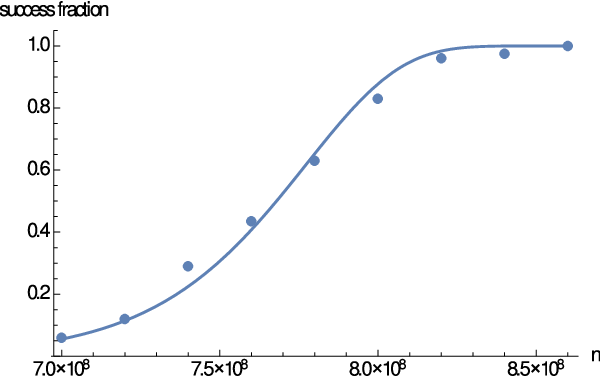
To empirically test the Karmarkar-Karp algorithm in a regime relevant to the cosmological constant problem, we generated random instances of the number partitioning problem, at various values of in which each of the numbers are independently sampled uniformly from . In figure 4, we plot the fraction of instances on which the Karmarkar-Karp algorithm was successful with numbers, where we defined success as achieving residue less than . In the context of finding small cosmological constant within the ADK model, one starts with real numbers of order 1, and seeks to find a residue of order . Here we have scaled up the numbers by a factor of and represented them as integers. This use of fixed-point arithmetic is strictly for computational convenience. Our definition of success corresponds to achieving a residue which is smaller than the magnitude of the initial numbers by a factor of and thus corresponds to finding a cosmological constant close to that observed for our universe44 4 A more precise match to our universe would be to seek a factor of , but this was not convenient to work with because it put the memory requirements of the algorithm just slightly beyond the available 128G of RAM on most of our computers. Achieving a factor requires and correspondingly an increase in time and memory cost of less than .. The extra 30 bits of precision are to ensure that “numerical noise” should be small.
By the analysis of [51], if the Karmarkar-Karp algorithm is applied to real numbers uniformly distributed on , the size of the final residue should be exponentially distributed. That is, the probability that the residue lies between and should be , where
| (18) |
and asymptotically equal to as . Empirical studies at finite consistently observe values of smaller than [51]. By defining success to be a reduction factor of , we should obtain success probability
| (19) | |||||
| (20) |
As one can see from figure 4, the observed success fraction from our trials of the Karmarkar-Karp algorithm on random instances agrees well with this prediction if we take .
IV.2 Sieves
The predicted work of a sieve to produce a residue of length is not so large that the universe would be unable to compute it, but it is large enough to require significant effort with current hardware. As a simple proof of concept, we will tackle a scaled down version with four sieve stages of block sizes , and use a simple meet-in-the-middle algorithm () to solve the number partitioning problem [60]. The profile of this experiment is as follows, which predicts an expected size of the final residue output at sieve stage four to be .
| Stage | Inputs | Distribution | #NPPs | Work | ||
|---|---|---|---|---|---|---|
| One | 1200000 | Uniform | 60000 | |||
| Two | 60000 | Exponential | 2000 | |||
| Three | 2000 | Exponential | 50 | |||
| Four | 50 | Exponential | 1 |
The result of the experiment is captured in figure 5.
Acknowledgements
We would like to thank Scott Aaronson, Adam Bouland, and Liam McAllister for discussions. N.B. is supported in part by the DuBridge Fellowship of the Walter Burke Institute for Theoretical Physics. R.B. is supported in part by the Berkeley Center for Theoretical Physics, by the National Science Foundation (award numbers PHY-1521446, PHY-1316783), by FQXi, and by the US Department of Energy under contract DE-AC02-05CH11231. S.J. and B.L. thank U. Maryland for use of the Deepthought2 high performance computing cluster. Parts of this manuscript are a contribution of NIST, an agency of the US government, and are not subject to US copyright.
References
- [1] S. Perlmutter et al. Measurements of Omega and Lambda from 42 high-redshift supernovae. Astrophys. J., 517:565–586, 1999.
- [2] Adam G. Riess et al. Observational evidence from supernovae for an accelerating universe and a cosmological constant. Astron. J., 116:1009–1038, 1998.
- [3] P. A. R. Ade et al. Planck 2015 results. XIII. Cosmological parameters. Astron. Astrophys., 594:A13, 2016.
- [4] Joseph Polchinski. The cosmological constant and the string landscape. arXiv:hep-th/0603249, 2006.
- [5] Raphael Bousso. TASI Lectures on the Cosmological Constant. Gen. Rel. Grav., 40:607–637, 2008.
- [6] R. Bousso and J. Polchinski. Quantization of four-form fluxes and dynamical neutralization of the cosmological constant. Journal of High Energy Physics, page 006, 2000. arXiv:hep-th/0004134.
- [7] G. W. Gibbons and S. W. Hawking. Cosmological event horizons, thermodynamics, and particle creation. Phys. Rev. D, 15:2738–2751, 1977.
- [8] Raphael Bousso. A covariant entropy conjecture. JHEP, 07:004, 1999.
- [9] Steven Weinberg. Anthropic bound on the cosmological constant. Phys. Rev. Lett., 59:2607, 1987.
- [10] Raphael Bousso, Ben Freivogel, Stefan Leichenauer, and Vladimir Rosenhaus. A geometric solution to the coincidence problem, and the size of the landscape as the origin of hierarchy. Phys. Rev. Lett., 106:101301, 2011.
- [11] Frederik Denef and Michael R. Douglas. Computational complexity of the landscape I. Annals of Physics, 322:1096–1142, 2007. arXiv:hep-th/0602072.
- [12] N. Arkani-Hamed, S. Dimopoulos, and S. Kachru. Predictive landscapes and new physics at a TeV. arXiv:hep-th/0501082, 2005.
- [13] Narendra Karmarkar, Richard M. Karp, George S. Leuker, and Andrew M. Odlyzko. Probabilistic analysis of optimum partitioning. Journal of Applied Probability, 23:626–645, 1986.
- [14] Stephan Mertens. Random costs in combinatorial optimization. Physical Review Letters, 84(6):1347, 2000.
- [15] Heiko Bauke, Silvio Franz, and Stephan Mertens. Number partitioning as a random energy model. Journal of Statistical Mechanics: Theory and Experiment, 2004(04):P04003, 2004.
- [16] Raphael Bousso. Complementarity in the Multiverse. Phys. Rev., D79:123524, 2009.
- [17] Raphael Bousso and Leonard Susskind. The Multiverse Interpretation of Quantum Mechanics. Phys.Rev., D85:045007, 2012.
- [18] Hans Moravec. Mind Children. Harvard University Press, 1990.
- [19] Scott Aaronson. NP-complete problems and physical reality. ACM SIGACT News, 36(1):30–52, 2005. arXiv:quant-ph/0502072.
- [20] Adam R. Brown, Daniel A. Roberts, Leonard Susskind, Brian Swingle, and Ying Zhao. Complexity, action, and black holes. Phys. Rev., D93(8):086006, 2016.
- [21] Seth Lloyd. Computational capacity of the universe. Physical Review Letters, 88:237901, 2002. arXiv:quant-ph/0110141.
- [22] Raphael Bousso. Holography in general space-times. JHEP, 06:028, 1999.
- [23] Raphael Bousso. Positive vacuum energy and the N-bound. JHEP, 11:038, 2000.
- [24] Raphael Bousso, Roni Harnik, Graham D. Kribs, and Gilad Perez. Predicting the cosmological constant from the causal entropic principle. Phys. Rev. D, 76:043513, 2007.
- [25] Scott Aaronson and John Watrous. Closed timelike curves make quantum and classical computing equivalent. Proceedings of the Royal Society A, 465(2102):631–647, 2009. arXiv:0808.2669.
- [26] Charles H. Bennett, Debbie Leung, Graeme Smith, and John A. Smolin. Can closed timelike curves or nonlinear quantum mechanics improve quantum state discrimination or help solve hard problems? Physical Review Letters, 103:170502, 2009. arXiv:0908.3023.
- [27] Todd A. Brun and Mark M. Wilde. Simulations of closed timelike curves. Foundations of Physics, 47(3):375–391, 2017. arXiv:1504.05911.
- [28] Daniel S. Abrams and Seth Lloyd. Nonlinear quantum mechanics implies polynomial-time solution for NP-complete and #p problems. Physical Review Letters, 81(18):3992, 1998. arXiv:quant-ph/9801041.
- [29] Ning Bao, Adam Bouland, and Stephen P. Jordan. Grover search and the no-signaling principle. Phys. Rev. Lett., 117(12):120501, 2016.
- [30] Frederik Denef, Michael R. Douglas, Brian Greene, and Claire Zukowski. Computational complexity of cosmology in string theory. Talk given by M. R. Douglas at JHS 75, Caltech, November 2016. Slides and video available at https://burkeinstitute.caltech.edu/workshops/JHS75 . Talk given by M. R. Douglas at “New Horizons in Inflationary Cosmology,” Stanford SITP, March 2017. Slides and video available at https://sitp.stanford.edu/conferences/new-horizons-inflationary-cosmology.
- [31] Frederik Denef, Michael R. Douglas, Brian Greene, and Claire Zukowski. Computational complexity of the landscape II – cosmological considerations. arXiv:1706.06430, 2017.
- [32] Daniel Harlow and Patrick Hayden. Quantum Computation vs. Firewalls. JHEP, 06:085, 2013.
- [33] Ning Bao, Adam Bouland, Aidan Chatwin-Davies, Jason Pollack, and Henry Yuen. Rescuing Complementarity With Little Drama. JHEP, 12:026, 2016.
- [34] A. Becker, J.-S. Coron, and A. Joux. Improved generic algorithms for hard knapsacks. In Advances in Cryptology–EUROCRYPT 2011, volume 6632 of LNCS, pages 364–385. Springer, 2011.
- [35] Daniel J. Bernstein, Stacey Jeffery, Tanja Lange, and Alexander Meurer. Quantum algorithms for the subset-sum problem. In PQCrypto 2013: Post-Quantum Cryptography 2013, volume 7932 of LNCS, pages 16–33. Springer, 2013.
- [36] Shamit Kachru, Renata Kallosh, Andrei Linde, and Sandip P. Trivedi. De Sitter vacua in string theory. Phys. Rev. D, 68:046005, 2003.
- [37] Michael R. Douglas and Shamit Kachru. Flux compactification. 2006.
- [38] Christos Papadimitriou. Computational Complexity. Pearson, 1993.
- [39] Richard M. Karp. Reducibility among combinatorial problems. In Raymond E. Miller, James W. Thatcher, and Jean D. Bohlinger, editors, Complexity of Computer Computations, pages 85–103. Springer US, Boston, MA, 1972.
- [40] Stephen Cook. The complexity of theorem proving procedures. In Proceedings of the third annual ACM Symposium on Theory of Computing (STOC), pages 151–158, 1971.
- [41] Vlatko Vedral, Adriano Barenco, and Artur Ekert. Quantum networks for elementary arithmetic operations. Physical Review A, 54:147–153, 1996.
- [42] Thomas G. Draper. Addition on a quantum computer. arXiv:quant-ph/0008033, 2000.
- [43] Thomas Draper, Samuel A. Kutin, Eric M. Rains, and Krysta M. Svore. A logarithmic-depth quantum carry-lookahead adder. Quantum Information and Computation, 6:351–369, 2006. arXiv:quant-ph/0406142.
- [44] Steven A. Cuccaro, Thomas G. Draper, Samuel A. Kutin, and David Petrie Moulton. A new quantum ripple-carry addition circuit. arXiv:quant-ph/0410184, 2004.
- [45] Yasuhiro Takahashi, Seiichiro Tani, and Noboru Kunihiro. Quantum addition circuits and unbounded fan-out. Quantum Information and Computation, 10:872–890, 2010.
- [46] Feng Wang, Minxing Luo, Huiran Li, Ziguo Qu, and Xiaojun Wang. Improved quantum ripple-carry addition circuit. Science China Information Sciences, 59:042406, 2016.
- [47] Robert W. Doran. The Gray code. Journal of Universal Computer Science, 13(11):1573–1597, 2007.
- [48] Rémi Monasson, Riccardo Zecchina, Scott Kirkpatrick, Bart Selman, and Lidror Troyansky. Determining computational complexity from characteristic phase transitions. Nature, 400:133–137, 1999.
- [49] Stefan Mertens. Phase transition in the number partitioning problem. Physical Review Letters, 81:4281, 1998. arXiv:cond-mat/9807077.
- [50] B. Yakir. The differencing algorithm LDM for partitioning: A proof of a conjecture of Karmarkar and Karp. Mathematics of Operations Research, 21:85–99, 1996.
- [51] Stefan Boettcher and Stephan Mertens. Analysis of the Karmarkar-Karp differencing algorithm. European Physics Journal B, 65:131–140, 2008. arXiv:0802.4040.
- [52] Thomas H. Cormen, Charles E. Leiserson, Ronald L. Rivest, and Clifford Stein. Introduction to Algorithms. MIT Press, 3rd edition, 2009.
- [53] Richard E. Korf. A complete anytime algorithm for number partitioning. Artificial Intelligence, 106(2):181–203, 1998.
- [54] W. Ruml, J. T. Ngo, J. Marks, and S. M. Schieber. Easily searched encodings for number partitioning. Journal of Optimization Theory and Applications, 89(2):251–291, 1996.
- [55] D. S. Johnson, C. R. Aragon, L. A. McGeoch, and C. Schevron. Optimization by simulated annealing: an experimental evaluation; part II, graph coloring and number partitioning. Operations Research, 39(3):378–406, 1991.
- [56] M. F. Arguello, T. A. Feo, and O. Goldshmidt. Randomized methods for the number partitioning problem. Computers and Operations Research, 23(2):103–111, 1996.
- [57] R. E. Berretta, P. Moscato, and C. Cotta. Enhancing a memetic algorithms’ performance using a matching-based recombination algorithm: results on the number partitioning problem. In M. G. C. Resende and J. Souza, editors, Metaheuristics: computer decision-making, pages 65–90. Kluwer Academic Publishers, 2004.
- [58] Michael R. Garey and David S. Johnson. Computers and Intractability: A guide to the theory of NP-completeness. W. H. Freeman, 1979.
- [59] Stephan Mertens. The easiest hard problem: number partitioning. In A. Percus, G. Istrate, and C. Moore, editors, Computational Complexity and Statistical Physics, chapter 5. Oxford University Press, 2006. arXiv:cond-mat/0310317.
- [60] Ellis Horowitz and Sartaj Sahni. Computing partitions with applications to the knapsack problem. Journal of the ACM (JACM), 21(2):277–292, 1974.
- [61] Vasil S. Denchev, Sergio Boixo, Sergei V. Isakov, Nan Ding, Ryan Babbush, Vadim Smelyanskiy, John Martinis, and Hartmut Neven. What is the computational value of finite-range tunneling? Physical Review X, 6:031015, 2016. arXiv:1512.02206.
- [62] Miklós Ajtai, Ravi Kumar, and Dandapani Sivakumar. A sieve algorithm for the shortest lattice vector problem. In Proceedings of the thirty-third annual ACM symposium on Theory of computing, pages 601–610. ACM, 2001.
- [63] Daniele Micciancio and Panagiotis Voulgaris. Faster exponential time algorithms for the shortest vector problem. In Proceedings of the twenty-first annual ACM-SIAM symposium on Discrete Algorithms, pages 1468–1480. SIAM, 2010.
- [64] Feng Zhang, Yanbin Pan, and Gengran Hu. A three-level sieve algorithm for the shortest vector problem. In International Conference on Selected Areas in Cryptography, pages 29–47. Springer, 2013.
- [65] Anja Becker, Nicolas Gama, and Antoine Joux. A sieve algorithm based on overlattices. LMS Journal of Computation and Mathematics, 17(A):49–70, 2014.
- [66] Thijs Laarhoven and Benne de Weger. Faster sieving for shortest lattice vectors using spherical locality-sensitive hashing. In International Conference on Cryptology and Information Security in Latin America, pages 101–118. Springer, 2015.
- [67] Anja Becker, Nicolas Gama, and Antoine Joux. Speeding-up lattice sieving without increasing the memory, using sub-quadratic nearest neighbor search. IACR Cryptology ePrint Archive, 2015:522, 2015.
- [68] Shi Bai, Thijs Laarhoven, and Damien Stehlé. Tuple lattice sieving. ANTS-XII (to appear), 2016.