Functionalizing Fe adatoms on Cu(001) as a nanoelectromechanical system
Abstract
This study demonstrates how the spin quantum dynamics of a single Fe atom adsorbed on Cu(001) can be controlled and manipulated by the vibrations of a nearby copper tip attached to a nano cantilever by virtue of the dynamic magnetic anisotropy. The magnetic properties of the composite system are obtained from ab initio calculations in completely relaxed geometries and turned out to be dependent considerably on the tip-iron distance that changes as the vibrations set in. The level populations, the spin dynamics interrelation with the driving frequency, as well as quantum information related quantities are exposed and analyzed.
1 Introduction
Microelectromechanical (MEMS) or nanoelectromechanical systems (NEMS) are at the verge of the classical-quantum world [1, 2, 3, 4] and can thus sense, possibly coupled, quantum-classical properties. For instance, tiny vibrating cantilever were shown to detect a single spin [5]. The sensitivity depends on the mean phonon number with the cantilever dynamics turning quantum as the phonons number decreases. Related to these observations, this field promises a new rout to quantum information nanomechanical devices. An example is the setup consisting of a single nitrogen-vacancy (NV) centre in a diamond nanocrystal deposited at the extremity of a SiC nanowire [6]. The quantum NV spin dynamics is observed to be coupled to the nanomechanical oscillator by means of the time-resolved nanocrystal fluorescence and photon-correlation measurements. This dynamic can be influenced by external fields such as a non-homogeneous magnetic field. A clear advantage of utilizing the spin-degrees of freedom of the NV is their long decoherence times even at room temperatures [7, 8, 9, 10, 11, 12]. Further phenomena emerge when considering strongly coupled nonlinear NEMS in which case phenomena such as nonlinear resonances can be exploited for the control of the energy transfer between the coupled NEMS [13, 14, 15, 16].
In the present work we propose a new type of NEMS based on a single magnetic Fe adatom deposited on a Cu(001) substrate. A proper choice of the driving frequency allows controlling the level populations in the system. The proposed (scanning-tunneling microscopy) STM-type or (atomic force microscopy) AFM-type setup is thus a hybrid system utilizing the quantum nature of single adsorbed atoms or molecules on the surface, which were designed as studied in an impressively controllable way experimentally (for example in Refs. [17, 18, 19]). The magnetic properties of Fe and Co adatoms on a Cu2N/Cu(100)-c surface were determined experimentally via x-ray magnetic dichroism measurements [20].
The possibly classical cantilever dissipative dynamics is coupled the quantum spin dynamics of the adsorbates since, as demonstrated below, the magnetic anisotropy is affected by the tip-adsorbate distance, and hence by the tip vibrational motion. This coupling might be exploited to access the topology or the local magnetic properties of spin systems [21].
2 Theoretical framework
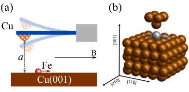
Specifically, we consider a single magnetic Fe atom deposited on a Cu(001) surface. A similar setup consisting of Fe or Mn on copper coated by an N overlayer, was shown to have a large magnetic anisotropy and relaxation times[22, 17]. Our calculations are carried out in the presence of a tip apex as in AFM experiments and reveal a substantial dependence of the magnetic anisotropy on the distance between the tip and the Fe adatom. Thus, in the proposed setup the magnetic properties of the single-atom are coupled to the oscillations of a nano-sized cantilever carrying the tip apex (FIG. 1(a)). As the characteristic frequencies of such nano-mechanical oscillators are known to reach the gigahertz regime[23], frequencies in the range of 100 GHz become feasible upon a further downscaling of the cantilever and can thus match the typical energy scale of the spin system (which is in the range of few meV).
3 ab initio calculations
Ab initio density-functional calculations of the ground state and the energy difference upon changing the magnetization axis of the Fe atom were performed using the projector augmented-wave (PAW) technique [24, 25], as implemented in the Vienna ab initio simulation package (VASP) [26]. The calculations are based on density-functional theory with the generalized gradient approximation (GGA) [27, 28]. We used the same methodology used in previous calculations of the magnetic anisotropy of Co and Fe adatoms on Rh(111), Pt(111) and Cu(100) substrates [29, 30, 31]. We note in this context that STM experiments were performed after the tip were in contact with the surface, and hence the tip is most likely covered by the surface material [32]. In this case a tip with surface atoms is often used in computer calculations [33, 34].
Our computational models consists 125 copper atoms representing the surface, the iron atom, and 5 additional atoms for simulating the presence of a tip apex, as depicted in FIG. 1(b). The unit cell has a size of 12.87 Å in the and directions (parallel to the surface), whereas the extent of the direction (perpendicular to the surface) amounts to 31.89 Å. At this slab thickness, the interaction between the tip and the repeated image of the surface is negligible. A cutoff energy of 300 eV is used. The calculations including spin-orbit coupling require a fine k-point mesh for the Brillouin-zone integrations. Test calculations were performed for iron atom on a Cu(001) surface for three different k-point grids: , , and generated by the Monkhorst-Pack scheme [35], in conjunction with a modest Gaussian smearing method. A grid provided the best compromise between accuracy and computational efforts.
The calculations were performed in two steps. First the coordinates of the iron atom and the positions of the atoms in the three topmost layers of the substrate (apart from the tip) were optimized using scalar-relativistic calculations until the forces on all unconstrained atoms were converged to less than 0.01 eV/Å. In the second step, the geometry and the electronic and magnetic ground states resulting from the scalar-relativistic calculations were used to initialize the relativistic calculations including spin-orbital coupling. Recent work [36] demonstrated that relaxations of Fe and Co adatom on Pt(111) with and without spin-orbit coupling are almost identical.
After a geometry optimization of the full cluster (apart from the tip) for every position of the tip, we computed the magnetic anisotropy energy as the difference of the respective ground state energies upon varying the magnetization axis. We found that the dependence on the angle measured from the Fe-tip axis is well described by the lowest-order anisotropy term , as it is known for similar systems. The dependence on the angle measured along the plane on the other hand turned out to be rather weak. Furthermore, we analyzed the spin density to investigate the degree of localization of the magnetization. The result is presented in FIG. 2 for small values of the density in two characteristic planes along the symmetry directions. We conclude that the Fe atom slightly polarizes the tip and the substrate below. Especially for the latter we observe the typical behavior of a spin density associated with this kind of anisotropy.
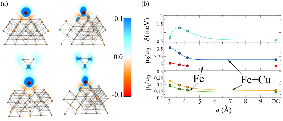
However, the major contribution to the magnetization is confined within the direct vicinity of the Fe atom, confirming that the effective surface spin can be interpreted as the magnetic moment of few atoms.
4 Modeling the spin dynamics
In FIG. 2(b) we show our results for the dependence of the magnetic anisotropy parameter and of the magnetic moments associated with the spin (), and the angular momentum () for four different values of the distance between the last tip atom and the iron atom. The spin magnetic moment on the iron atom without the tip-adatom interaction is 2.94 . This result agrees well with previous density functional calculations [37]. It should be noted, that the magnetic anisotropy parameter for an atom on the surface is very sensitive to the interatomic distances [38, 39] and the arrangement of the atom [29, 40]. It was demonstrated that the structural relaxation of the adatom and the substrate reduces significantly the magnetic anisotropy energy [38, 39]. Therefore, compared to ab initio calculations for the Fe adatom on the ideal Cu(001) surface, our magnetic anisotropy energy obtained in a fully relaxed geometry is several times less than the value presented in Ref. [41].
Based on the fitting functions displayed in FIG. 2(b) we are now able to formulate the Hamiltonian describing the effective surface angular momentum with the parametric dependence on as
| (1) |
We assume a magnetic field with a strength is applied along the axis. Approximating the total angular momentum with 2 turns out to be an adequate description and can be confirmed experimentally by means of inelastic tunneling spectroscopy [22, 17]. The distance-dependent gyromagnetic ratios for spin (angular) momentum () account for the varying magnitude of the total magnetic moment (see Fig. 2(b)), as extracted from our ab initio calculations. We fix to the value of 4 T and take the ground state as the initial state. As one can readily show for eq. (1), the expectation value with respect to all eigenstates of and is exactly zero. This holds true even for the case of the time-dependent Schrödinger equation, when replacing .
To map out the spin dynamics for a representative case we choose by and T. The energies of the eigenstates (on the ordinate axis) and the expectation values of (abscissa) are shown in the inset in FIG. 3. For a high density of phonons the spin dynamics originates from an oscillation of the tip apex according to for (we assume for ). This corresponds to a setup where the system is initially in its ground state and is driven out of equilibrium by the cantilever oscillations for . The oscillation amplitude is chosen as Å.
Before discussing the results, let us elaborate on the qualitative aspects of the dynamics. Since the spin is driven by an effectively time-dependent anisotropy, i. e. the coupling to the operator , the induced transitions allow for changing the spin projection only. The magnetic moment will thus remain parallel to . Therefore, only the longitudinal spin dynamics can be induced, limiting the transitions from the ground state to only the two excited states that match in symmetry.
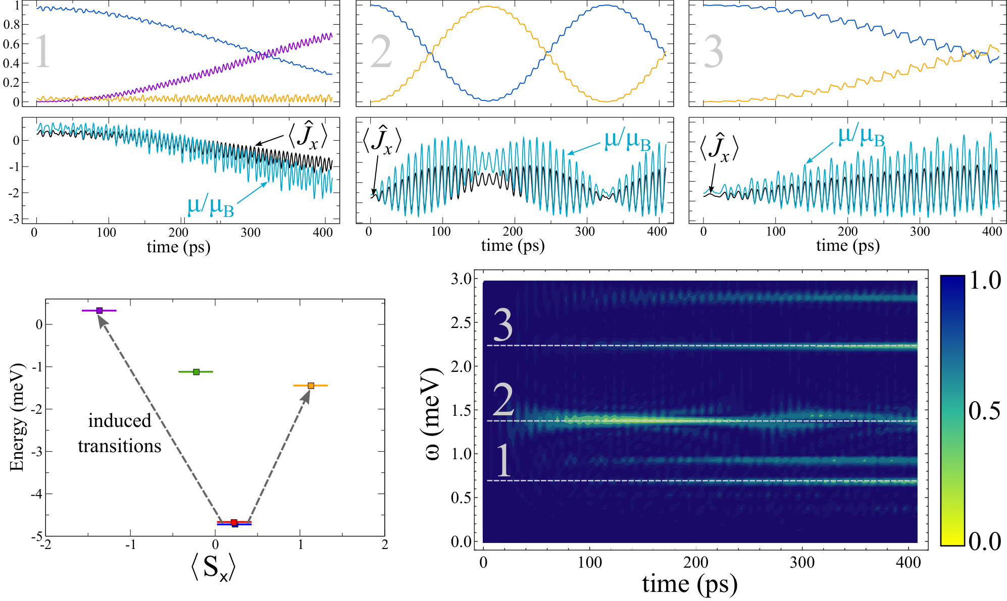
In FIG. 3 we present the resulting spin dynamics in dependence on . The color map plot (lower right figure) shows the population of the ground state (which we have chosen as the initial state). Interestingly, the magnetic moment is hardly affected by the variation of the magnetic anisotropy for the major part of the frequency range. Apart from that, a couple of distinct lines indicate an optimal setting for the parameters to drive the angular momentum to some excited states. A more detailed analysis reveals that the dynamics for the frequencies indicated by the dashed lines (labelled by 1,2,3) exhibits almost Rabi-like transitions from the ground state to a single excited state. This behavior can be explored further by a Floquet analysis. We therefore expand the angular momentum wave function as
| (2) |
where are the quasi energies and the Floquet eigenvectors. Both can be obtained by solving the eigenvalue problem of the time-evolution operator at , since
| (3) |
(note that ). Before discussing the solution of eq. (3), let us briefly revisit how the dynamics shown in FIG. 3 can be explained within the Floquet theory. Eq. (2) expresses the expansion of the time-dependent spin state in terms of the orthonormal Floquet states , with the projection coefficients . For the case , the projection amounts to , such that the population of the initial state remains one at multiples of . Assuming on the other hand yields the stroboscopic time evolution
| (4) |
These two scenarios explain the dynamics observed in FIG. 3, where slow, Rabi-like population transfer (with a frequency corresponding to the difference of two quasienergies) is overlayed with fast oscillations (which originate from the overlaps of the type and are thus periodic with the frequency ). The quasienergies obtained from eq. (3) are presented in FIG. 4(a) (upper panel), along with the projection (lower panel). As pointed out, the decisive factor for the depletion of the ground state is at least two projection coefficients being different from zero. For this reason, we have ordered the quasienergies according to the magnitude of . As it turned out, only two of the Floquet states display a significant contribution to the initial state. Therefore, only their projection is shown in FIG. 4(a). For the complete picture of the behaviour of the quasienergies however, the third state and its eigenvalue are included in the upper panel.
The vertical lines in FIG. 4(a) demonstrate that the scenario for the dynamics according to eq. (4) occurs only at the crossing points of the quasienergies, where (at least) two branches exchange their character, that is the magnitude of their projection coefficients. A more detailed analysis reveals that all crossings are avoided crossings. The difference of the quasienergies becomes thus relatively small, leading to the slow dynamics in FIG. 3. For the exemplary values of , FIG. 4(b)–(c) provides a magnification of the crossing points and gives their width. Converting the quasienergy gap into a time scale results in exactly the characteristic time of the slow dynamics in FIG. 3.
5 Entanglement measures
With cooling down the system, oscillations of the nanocantilever become inherently quantum. Thus the nanocantilever can detect inter-level transitions of the single spin. This statement is generic for a broad class of the nanomechanical systems and is valid for our model as well. Our model is exactly solvable (which is in fact its merit) and allow to explore analytically the entanglement between the cantilever and the system. In contrast to the above, where we investigated the case of a moderate elongations of the cantilever, leading to a nonlinear coupling, we consider linear coupling only. In addition to the feasibility of analytical solutions, the quantum fluctuations and the oscillations of the cantilever occur on a smaller scale, while large elongations are associated with the classical case which is studied above.
In order to quantify the entanglement in the system, we explore von Neumann entropy. In the quantum information theory the von Neumann entropy is known as the ”entanglement entropy” of the reduced density matrix. The technical details of the von Neumann entropy and hence of the reduced density matrix in our case are given in Appendix A.
To construct a quantized model, the tip-substrate distance is replaced by , where () is the creation (annihilation) operator of the cantilever modes. Modern technologies enabled the fabrication of dual mode () cantilevers, for more details see [42, 43].
The resulting Hamiltonian, in lowest order in the oscillation amplitude reads
Similar to the classical case analyzed above, the transition operator allows the transition from the ground state to two excited states only. Hence, the Hamiltonian (5) can be reduced to a three-level system in spin space. We assume that the cantilever frequencies match the excitation energies .
We solve directly analytically for the Schrödinger equation
| (5) |
using the following ansatz
| (6) | |||||
Here quantify the number of phonons in the cavity with the frequencies . Taking into account Eq. (5), (6) we consider the resonance condition , . After standard calculations we obtain
| (7) | |||||
| (8) | |||||
In Eq. (7) and (8) we introduced the notation . Further simplifications enabling an analytical treatment are giving rise to the effective coupling constant .
While the solution Eq. (6)-(8) is obtained for a fixed value of the magnetic field T, it is valid for an arbitrary field. Changing the magnetic field rescales the level spacing, thus leading to a slight rescaling of the Rabi-like transition frequencies.
The quantities we are interested in, such as level populations and von Neumann entropy (where is the density matrix of the system) can be calculated directly from (7) and (8). For this purpose we need to consider the averaging of Eq. (7)–(8) over the phonon distribution functions for the coherent states . Here is the mean phonon number corresponding to the classical limit.
For the calculations of the average level populations we perform summation over the phonon numbers and :
| (9) |
The coefficients have a sharp maximum near the mean phonon numbers , and the width of their distribution is rather small . This allows performing the summation analytically and obtaining expressions for the level populations and for the von Neumann entropy. The explicit expression is presented in A.
With the analytical solutions at hand, we can now study the population dynamics and the von Neumann entropy of the spin system due to the interaction with the cantilever. FIG. 5 depicts this dynamics with an oscillation amplitude of Å. Due to the strong dependence of the anisotropy on the tip-sample distance, the dynamics at Å (FIG. 5(a)) and Å (FIG. 5(b)) occurs on very different time scales. We clearly see that quantum revivals in level populations are synchronized with the sudden death of von Neumann entropy. This behavior is more prominent in the case of a strong coupling (FIG. 5(a)). Obviously with the increase of the phonon number the period of quantum revivals becomes larger. In the limit of the classical field the revival time tends to infinity. Meaning that the classical field like thermal bath thermalizes the system and leads to irreversibility.
6 Conclusions
In summary, we performed ab initio calculations of the magnetic properties of a single Fe atom adsorbed on Cu(001). We demonstrated that the electronic and the magnetic properties of adatoms are strongly affected by the tip-surface distance. Based on these results we proposed a new type of NEMS consisting of a single magnetic Fe adatoms deposited on a Cu(001) substrate and analyzed its fundamental properties and possible operation scheme.
Appendix A von Neumann entropy
Acknowledgments
AK acknowledges the financial support by the joint program of MSU-DAAD Vladimir Vernadsky (A/12/89268) and Volnoe Delo foundation . Computational resources were provided by the Supercomputing Center of Lomonosov Moscow State University. The work was partially funded by the German Science Foundation under SFB 762.
References
References
- [1] Chan J, Alegre T P M, Safavi-Naeini A H, Hill J T, Krause A, Gröblacher S, Aspelmeyer M and Painter O 2011 Nature 478 89–92
- [2] Ludwig M, Hammerer K and Marquardt F 2010 Phys. Rev. A 82(1) 012333 URL http://link.aps.org/doi/10.1103/PhysRevA.82.012333
- [3] Heinrich G and Marquardt F 2011 EPL (Europhysics Letters) 93 18003 URL http://stacks.iop.org/0295-5075/93/i=1/a=18003
- [4] Hammerer K, Wallquist M, Genes C, Ludwig M, Marquardt F, Treutlein P, Zoller P, Ye J and Kimble H J 2009 Phys. Rev. Lett. 103(6) 063005 URL http://link.aps.org/doi/10.1103/PhysRevLett.103.063005
- [5] Rugar D, Budakian R, Mamin H J and Chui B W 2004 Nature 430 329–332
- [6] Arcizet O, Jacques V, Siria A, Poncharal P, Vincent P and Seidelin S 2011 Nature Phys. 7 879–883
- [7] Rabl P, Cappellaro P, Dutt M V G, Jiang L, Maze J R and Lukin M D 2009 Phys. Rev. B 79(4) 041302 URL http://link.aps.org/doi/10.1103/PhysRevB.79.041302
- [8] Treutlein P 2012 Nature 335 1584–1585
- [9] Mishra S K, Chotorlishvili L, Rau A R P and Berakdar J 2014 Phys. Rev. A 90(3) 033817 URL http://link.aps.org/doi/10.1103/PhysRevA.90.033817
- [10] Jelezko F, Gaebel T, Popa I, Gruber A and Wrachtrup J 2004 Phys. Rev. Lett. 92(7) 076401 URL http://link.aps.org/doi/10.1103/PhysRevLett.92.076401
- [11] Fuchs G D, Dobrovitski V V, Toyli D M, Heremans F J and Awschalom D D 2009 Nature 326 1520–1522
- [12] Chotorlishvili L, Sander D, Sukhov A, Dugaev V, Vieira V R, Komnik A and Berakdar J 2013 Phys. Rev. B 88(8) 085201 URL http://link.aps.org/doi/10.1103/PhysRevB.88.085201
- [13] Karabalin R B, Cross M C and Roukes M L 2009 Phys. Rev. B 79(16) 165309 URL http://link.aps.org/doi/10.1103/PhysRevB.79.165309
- [14] Chotorlishvili L, Ugulava A, Mchedlishvili G, Komnik A, Wimberger S and Berakdar J 2011 Journal of Physics B: Atomic, Molecular and Optical Physics 44 215402 URL http://stacks.iop.org/0953-4075/44/i=21/a=215402
- [15] Lifshitz R and Cross M C 2003 Phys. Rev. B 67
- [16] Bromberg Y, Cross M C and Lifshitz R 2006 Phys. Rev. E 73(1) 016214 URL http://link.aps.org/doi/10.1103/PhysRevE.73.016214
- [17] Loth S, Etzkorn M, Lutz C P, Eigler D M and Heinrich A J 2010 Science 329 1628–1630
- [18] Loth S, Baumann S, Lutz C P, Eigler D M and Heinrich A J 2012 Science 335 196–199
- [19] Schwöbel J, Fu Y, Brede J, Dilullo A, Hoffmann G, Klyatskaya S, Ruben M and Wiesendanger R 2012 Nature communications 3 953
- [20] Etzkorn M, Hirjibehedin C F, Lehnert A, Ouazi S, Rusponi S, Stepanow S, Gambardella P, Tieg C, Thakur P, Lichtenstein A I, Shick A B, Loth S, Heinrich A J and Brune H 2015 Phys. Rev. B 92(18) 184406 URL https://link.aps.org/doi/10.1103/PhysRevB.92.184406
- [21] Wolter B, Yoshida Y, Kubetzka A, Hla S W, von Bergmann K and Wiesendanger R 2012 Phys. Rev. Lett. 109
- [22] Hirjibehedin C F, Lin C Y, Otte A F, Ternes M, Lutz C P, Jones B A and Heinrich A J 2007 Science 317 1199–1203
- [23] Agarwal A K G S 2011 Mathematical and Computational Applications 16 290–300
- [24] Blöchl P E 1994 Phys. Rev. B 50(24) 17953–17979 URL http://link.aps.org/doi/10.1103/PhysRevB.50.17953
- [25] Kresse G and Joubert D 1999 Phys. Rev. B 59(3) 1758–1775 URL http://link.aps.org/doi/10.1103/PhysRevB.59.1758
- [26] Kresse G and Hafner J 1993 Phys. Rev. B 48(17) 13115–13118 URL http://link.aps.org/doi/10.1103/PhysRevB.48.13115
- [27] Wang Y and Perdew J P 1991 Phys. Rev. B 44(24) 13298–13307 URL http://link.aps.org/doi/10.1103/PhysRevB.44.13298
- [28] Perdew J P and Wang Y 1992 Phys. Rev. B 45(23) 13244–13249 URL http://link.aps.org/doi/10.1103/PhysRevB.45.13244
- [29] Błoński P, Lehnert A, Dennler S, Rusponi S, Etzkorn M, Moulas G, Bencok P, Gambardella P, Brune H and Hafner J 2010 Phys. Rev. B 81(10) 104426 URL http://link.aps.org/doi/10.1103/PhysRevB.81.104426
- [30] Kolesnikov S, Klavsyuk A and Saletsky A 2013 Surface Science 612 48 – 56 URL http://www.sciencedirect.com/science/article/pii/S0039602813000599
- [31] Klavsyuk A L, Kolesnikov S V and Saletsky A M 2014 JETP Letters 99 646–649 ISSN 1090-6487 URL http://dx.doi.org/10.1134/S0021364014110046
- [32] Hofer W A, Foster A S and Shluger A L 2003 Rev. Mod. Phys. 75(4) 1287–1331 URL https://link.aps.org/doi/10.1103/RevModPhys.75.1287
- [33] Kürpick U and Rahman T S 1999 Phys. Rev. Lett. 83(14) 2765–2768 URL https://link.aps.org/doi/10.1103/PhysRevLett.83.2765
- [34] Huang R Z, Stepanyuk V S, Klavsyuk A L, Hergert W, Bruno P and Kirschner J 2006 Phys. Rev. B 73(15) 153404 URL https://link.aps.org/doi/10.1103/PhysRevB.73.153404
- [35] Monkhorst H J and Pack J D 1976 Phys. Rev. B 13(12) 5188–5192 URL http://link.aps.org/doi/10.1103/PhysRevB.13.5188
- [36] Błoński P and Hafner J 2009 Journal of Physics: Condensed Matter 21 426001
- [37] Stepanyuk V S, Baranov A N, Hergert W and Bruno P 2003 Phys. Rev. B 68(20) 205422 URL http://link.aps.org/doi/10.1103/PhysRevB.68.205422
- [38] Pick i c v, Stepanyuk V S, Baranov A N, Hergert W and Bruno P 2003 Phys. Rev. B 68(10) 104410 URL http://link.aps.org/doi/10.1103/PhysRevB.68.104410
- [39] Pick i c v, Stepanyuk V S, Klavsyuk A L, Niebergall L, Hergert W, Kirschner J and Bruno P 2004 Phys. Rev. B 70(22) 224419 URL http://link.aps.org/doi/10.1103/PhysRevB.70.224419
- [40] Balashov T, Schuh T, Takács A F, Ernst A, Ostanin S, Henk J, Mertig I, Bruno P, Miyamachi T, Suga S and Wulfhekel W 2009 Phys. Rev. Lett. 102(25) 257203 URL http://link.aps.org/doi/10.1103/PhysRevLett.102.257203
- [41] Lazarovits B, Szunyogh L, Weinberger P and Újfalussy B 2003 Phys. Rev. B 68(2) 024433 URL http://link.aps.org/doi/10.1103/PhysRevB.68.024433
- [42] Chawla G and Solares S D 2009 Measurement Science and Technology 20 015501 URL http://stacks.iop.org/0957-0233/20/i=1/a=015501
- [43] Solares S D and Chawla G 2008 Measurement Science and Technology 19 055502 URL http://stacks.iop.org/0957-0233/19/i=5/a=055502