The partition function of a theory in CSM$(n)$ defined on $S^{3}$ can be given in terms of a finite-dimensional integral [13] as

$$Z\ =\ \int d^{N_{1}}u\,d^{N_{2}}w\,\exp\left[\frac{ik_{1}}{4\pi}\sum_{i=1}^{N_{1}}(u_{i})^{2}+\frac{ik_{2}}{4\pi}\sum_{a=1}^{N_{2}}(w_{a})^{2}\right]\frac{\prod_{i<j}^{N_{1}}(\sinh\frac{u_{i}-u_{j}}{2})^{2}\prod_{a<b}^{N_{2}}(\sinh\frac{w_{a}-w_{b}}{2})^{2}}{\prod_{i=1}^{N_{1}}\prod_{a=1}^{N_{2}}(\cosh\frac{u_{i}-w_{a}}{2})^{n}}.$$

(2.1)

This integral can be regarded as the partition function of a matrix model. As usual for matrix models, we may take the planar limit which makes the saddle point approximation for the integral (2.1) exact. The planar limit is defined by introducing an auxiliary parameter $k$ as

$$k\ \to\ \infty\hskip 14.22636pt\mbox{with }\hskip 14.22636ptt_{\alpha}\ :=\ \frac{2\pi iN_{\alpha}}{k},\hskip 14.22636pt\kappa_{\alpha}\ :=\ \frac{k_{\alpha}}{k}\hskip 14.22636pt\mbox{fixed.}\hskip 14.22636pt(\alpha=1,2)$$

(2.2)

In this limit, the integral in (2.1) is dominated by the saddle point which satisfies the following equations:

	$\displaystyle\frac{k_{1}}{2\pi i}u_{i}$	$\displaystyle=$	$\displaystyle\sum_{j\neq i}^{N_{1}}\coth\frac{u_{i}-u_{j}}{2}-\frac{n}{2}\sum_{a_{1}}^{N_{2}}\tanh\frac{u_{i}-w_{a}}{2},$		(2.3)
	$\displaystyle\frac{k_{2}}{2\pi i}w_{a}$	$\displaystyle=$	$\displaystyle\sum_{b\neq a}^{N_{2}}\coth\frac{w_{a}-w_{b}}{2}-\frac{n}{2}\sum_{i=1}^{N_{1}}\tanh\frac{w_{a}-u_{i}}{2}.$		(2.4)

Let $\{\bar{u}_{i},\bar{w}_{a}\}$ denote the solution of these equations. Because of the presence of $i$ in the left-hand side, $\bar{u}_{i}$ and $\bar{w}_{a}$ are complex numbers in general. For later convenience, the eigenvalues $\bar{u}_{i}$ and $\bar{w}_{a}$ are labeled such that

$${\rm Re}(\bar{u}_{i})\ \leq\ {\rm Re}(\bar{u}_{i+1}),\hskip 28.45274pt{\rm Re}(\bar{w}_{a})\ \leq\ {\rm Re}(\bar{w}_{a+1})$$

(2.5)

holds. We assume that both $\bar{u}_{i}$ and $\bar{w}_{a}$ approach zero in the small ’t Hooft coupling limit, since in this limit the left-hand sides dominate in the equations.

Some physical observables can be calculated in the planar limit. The free energy is obtained from the saddle point value of the integral (2.1). In addition, there are two BPS Wilson loops for ${\rm U}(N_{1})$ gauge fields and ${\rm U}(N_{2})$ gauge fields. Their vevs in the planar limit are given as

$$\langle W_{1}\rangle\ =\ \frac{1}{N_{1}}\sum_{i=1}^{N_{1}}e^{\bar{u}_{i}},\hskip 28.45274pt\langle W_{2}\rangle\ =\ \frac{1}{N_{2}}\sum_{a=1}^{N_{2}}e^{\bar{w}_{a}}.$$

(2.6)

The information of the theory in the planar limit is encoded in a row-vector-valued resolvent [30]

$$v(z)\ :=\ (v_{1}(z),v_{2}(z)).$$

(2.7)

The components $v_{\alpha}(z)$ are defined as

$$v_{1}(z)\ :=\ \lim\frac{t_{1}}{N_{1}}\sum_{i=1}^{N_{1}}\frac{z+e^{\bar{u}_{i}}}{z-e^{\bar{u}_{i}}},\hskip 28.45274ptv_{2}(z)\ :=\ \lim\frac{t_{2}}{N_{2}}\sum_{a=1}^{N_{2}}\frac{z-e^{\bar{w}_{a}}}{z+e^{\bar{w}_{a}}},$$

(2.8)

where $\lim$ indicates the planar limit (2.2). The function $v_{1}(z)$ has a square-root branch cut on an interval $I_{1}$ in $\mathbb{C}$, and holomorphic elsewhere, including the point at infinity. The branch points $a_{1}$ and $b_{1}$ on $I_{1}$ are given as

$$a_{1}\ :=\ e^{\bar{u}_{1}},\hskip 28.45274ptb_{1}\ :=\ e^{\bar{u}_{N_{1}}}.$$

(2.9)

Due to the symmetry of the equations (2.3)(2.4), they satisfy

$$a_{1}b_{1}\ =\ 1.$$

(2.10)

The other function $v_{2}(z)$ has similar properties. The branch points $a_{2}$ and $b_{2}$ are given as

$$a_{2}\ :=\ -e^{\bar{w}_{1}},\hskip 28.45274ptb_{2}\ :=\ -e^{\bar{w}_{N_{2}}}$$

(2.11)

which also satisfy

$$a_{2}b_{2}\ =\ 1.$$

(2.12)

Note that $|a_{\alpha}|\leq 1$ are satisfied.

The resolvent $v(z)$ is determined by specifying two complex parameters, say $a_{\alpha}$. These two parameters are related to the values of the ’t Hooft couplings $t_{\alpha}$ for given $\kappa_{\alpha}$ via

$$v(0)\ =\ -(t_{1},t_{2}).$$

(2.13)

It was found in [30] that it is convenient to investigate a derivative $zv^{\prime}(z)$ of the resolvent, instead of $v(z)$ itself, since the former can be obtained explicitly. In the following, we assume $n\neq 2$.

Let $c:=(c_{1},c_{2})$ be the row vector satisfying

$$(2\kappa_{1},2\kappa_{2})\ =\ (c_{1},c_{2})\left[\begin{array}[]{cc}2&-n\\ -n&2\end{array}\right].$$

(2.14)

Note that the solution of this equation exists for $n\neq 2$. Let us introduce another row-vector-valued function $f(z)$ such that $zv^{\prime}(z)$ can be written as

$$zv^{\prime}(z)\ =\ c+\frac{1}{s(z)}f(z),\hskip 28.45274pts(z)\ :=\ \sqrt{(z-a_{1})(z-b_{1})(z-a_{2})(z-b_{2})}.$$

(2.15)

In order to determine the explicit form of $f(z)$, we introduce a new variable $u$ defined as

$$u(z)\ :=\ \frac{\varphi(z)}{2\varphi(b_{1})},\hskip 28.45274pt\varphi(z)\ :=\ \int_{a_{1}}^{z}\frac{d\xi}{s(\xi)},$$

(2.16)

where the integration contour for $\varphi(b_{1})$ lies above the segment $I_{1}$. The saddle point equations (2.3)(2.4) imply that, as a function of $u$, $f(z)$ can be written as

$$f(z(u))\ =\ \left(\tilde{f}(u),\tilde{f}(-u)\right)S^{-1},\hskip 28.45274ptS\ :=\ \left[\begin{array}[]{cc}1&1\\ -e^{\pi i\nu}&-e^{-\pi i\nu}\end{array}\right]$$

(2.17)

where $\nu$ is related to $n$ by $n=2\cos\pi\nu$. The scalar function $\tilde{f}(u)$ is required to satisfy

$$\tilde{f}(u+1)\ =\ \tilde{f}(u),\hskip 28.45274pt\tilde{f}(u+\tau)\ =\ e^{2\pi i\nu}\tilde{f}(u)$$

(2.18)

where $\tau:=2u(a_{2})$. Therefore, $\tilde{f}(u)$ can be written in terms of the theta functions. The explicit form of $\tilde{f}(u)$ is given in Appendix A.

Since what we have obtained is $zv^{\prime}(z)$, the relation (2.13) cannot be used to determine $t_{\alpha}$ for a given $a_{\alpha}$. An alternative way to recover $t_{\alpha}$ is to use the formula

$$t_{\alpha}\ =\ -\frac{1}{2}\int_{C_{\alpha}}\frac{dz}{2\pi i}\frac{\log z}{z}zv_{\alpha}^{\prime}(z),$$

(2.19)

where $C_{1}$ ($C_{2}$) is a contour encircling the segment $I_{1}$ ($I_{2}$) counterclockwise.

In addition to $t_{\alpha}$, the expansion of $zv^{\prime}(z)$ provides the vevs $\langle W_{\alpha}\rangle$ of BPS Wilson loops as

$$zv^{\prime}(z)\ =\ -2\left(t_{1}\langle W_{1}\rangle,-t_{2}\langle W_{2}\rangle\right)z+O(z^{2}).$$

(2.20)

Combining (2.19) and (2.20), the vevs $\langle W_{\alpha}\rangle$ can be given as functions of $t_{\alpha}$.

Various quantities can be calculated perturbatively when the ’t Hooft couplings $t_{\alpha}$ are small. For example, the vevs $\langle W_{\alpha}\rangle$ are given as [30]

	$\displaystyle\langle W_{1}\rangle$	$\displaystyle=$	$\displaystyle 1+\frac{t_{1}}{2\kappa_{1}}+\frac{1}{6}\left(\frac{t_{1}}{\kappa_{1}}\right)^{2}\left(1-\frac{1}{4N_{1}^{2}}\right)-\frac{n}{8}\frac{t_{1}t_{2}}{\kappa_{1}^{2}}+O(t^{3}),$		(2.21)
	$\displaystyle\langle W_{2}\rangle$	$\displaystyle=$	$\displaystyle 1+\frac{t_{2}}{2\kappa_{2}}+\frac{1}{6}\left(\frac{t_{2}}{\kappa_{2}}\right)^{2}\left(1-\frac{1}{4N_{2}^{2}}\right)-\frac{n}{8}\frac{t_{1}t_{2}}{\kappa_{2}^{2}}+O(t^{3}),$		(2.22)

which can be obtained by using the method developed in [13]. This result was reproduced in [30] from the resolvent $v(z)$ reviewed above by using the formulas (2.19)(2.20) for cases when $N_{1}=N_{2}$ and $k_{1}=\pm k_{2}$ are satisfied. This can be regarded as a non-trivial check of the validity of the resolvent $v(z)$ obtained in [30].

The method in [13], however, does not give us any information on the configuration of the eigenvalues $\{\bar{u}_{i},\bar{w}_{a}\}$, and therefore, the positions $a_{\alpha}$ of the branch points of $v(z)$. To obtain such information, it is better to solve the saddle point equations (2.3)(2.4) perturbatively, as in [11].

In the following, we will restrict ourselves to the case $N_{1}=N_{2}=:N$ for simplicity. This implies that $t_{1}=t_{2}=:t$ holds. The analysis of this case should be the first step toward the understanding of the general case.

Recall that the saddle point equations in this case are

	$\displaystyle\frac{k_{1}}{2\pi i}u_{i}$	$\displaystyle=$	$\displaystyle\sum_{j\neq i}^{N}\coth\frac{u_{i}-u_{j}}{2}-\frac{n}{2}\sum_{a=1}^{N}\tanh\frac{u_{i}-w_{a}}{2},$		(2.23)
	$\displaystyle\frac{k_{2}}{2\pi i}w_{a}$	$\displaystyle=$	$\displaystyle\sum_{b\neq a}^{N}\coth\frac{w_{a}-w_{b}}{2}-\frac{n}{2}\sum_{i=1}^{N}\tanh\frac{w_{a}-u_{i}}{2}.$		(2.24)

Assume that $t$ is small, and introduce rescaled variables $x_{i}$ and $y_{a}$ defined such that

$$u_{i}\ =\ \sqrt{t}\,x_{i},\hskip 28.45274ptw_{a}\ =\ \sqrt{t}\,y_{a}$$

(2.25)

holds. Then, the saddle point equations can be expanded in $t$. The leading order terms give the following simple equations:

$$\kappa_{1}x_{i}\ =\ \frac{2}{N}\sum_{j\neq i}^{N}\frac{1}{x_{i}-x_{j}},\hskip 28.45274pt\kappa_{2}y_{a}\ =\ \frac{2}{N}\sum_{b\neq a}\frac{1}{y_{a}-y_{b}}.$$

(2.26)

Each of these equations are the same as the saddle point equations of the Gaussian matrix model. The planar solution of them is encoded in

	$\displaystyle\omega_{1}(z)\ :=\ \lim\frac{1}{N}\sum_{i=1}^{N}\frac{1}{z-x_{i}}\ =\ \frac{\kappa_{1}}{2}\left[z-\sqrt{z^{2}-\frac{4}{\kappa_{1}}}\ \right],$		(2.27)
	$\displaystyle\omega_{2}(z)\ :=\ \lim\frac{1}{N}\sum_{a=1}^{N}\frac{1}{z-y_{a}}\ =\ \frac{\kappa_{2}}{2}\left[z-\sqrt{z^{2}-\frac{4}{\kappa_{2}}}\ \right].$		(2.28)

The perturbative corrections to this solution can be systematically calculated, as shown in [11] for ABJM theory.

The discontinuity of $\omega_{1}(z)$ and $\omega_{2}(z)$ encodes the distributions of $\{x_{i}\}$ and $\{y_{a}\}$ which then give the distributions of $\{u_{i}\}$ and $\{w_{a}\}$. The definitions (2.9)(2.11) of the parameters $a_{1}$ and $a_{2}$ imply that they are given as

$$a_{1}\ \sim\ \exp\left(-2\sqrt{\frac{t}{\kappa_{1}}}\ \right),\hskip 28.45274pta_{2}\ \sim\ -\exp\left(-2\sqrt{\frac{t}{\kappa_{2}}}\ \right)$$

(2.29)

for small $t$.

One may notice that the relation between $a_{1}$ and $a_{2}$ becomes quite simple when $\kappa_{1}=\kappa_{2}$ holds. In this case, the parameters are related simply as

$$a_{1}\ =\ -a_{2}\ =:\ a.$$

(2.30)

This relation is satisfied when the equalities $\bar{u}_{i}=\bar{w}_{i}$ hold. Since this equality is compatible with the full saddle point equations (2.23)(2.24) with $k_{1}=k_{2}$, the relation (2.30) should hold beyond perturbation. Therefore, any observables which can be derived from the resolvent $v(z)$ are functions of $a$. Without loss of generality, we can choose $\kappa_{1}=\kappa_{2}=1$.

Note that the explicit form of $zv^{\prime}(z)$ shown in Appendix A is written in terms of the parameters $u_{0},u_{\infty}$, and $\tau$. The definition of $u(z)$ implies

$$u_{\infty}\ =\ u_{0}-\frac{1}{2}.$$

(2.31)

When the equality $a_{1}=-a_{2}$ holds, $u_{0}$ is given by $\tau$ as

$$u_{0}\ =\ \frac{1}{4}\tau.$$

(2.32)

Therefore, all the observables are also functions of $\tau$. The relation between $a$ and $\tau$ can be obtained from the inverse of $u(z)$ given as

$$z(u)\ =\ -\frac{\vartheta_{1}(u-u_{0})\vartheta_{1}(u+u_{0})}{\vartheta_{1}(u-u_{\infty})\vartheta_{1}(u+u_{\infty})}.$$

(2.33)

Since $z=a$ corresponds to $u=0$ by definition, $a$ is related to $\tau$ as

$$a\ =\ -\left(\frac{\vartheta_{1}(\frac{1}{4}\tau)}{\vartheta_{1}(\frac{1}{4}\tau-\frac{1}{2})}\right)^{2}.$$

(2.34)

In the following, we choose $\tau$ as the parameter specifying the resolvent.

It is important to notice that not all values of $\tau$ are physically relevant. Since the ’t Hooft couplings are defined as (2.2), their physical values are purely imaginary. Therefore, $\tau$ must be chosen such that the integrals (2.19) take purely imaginary values. The physical values of $\tau$ form a curve $\gamma$ in the complex $\tau$-plane.

The asymptotic behavior of $\gamma$ in the small ’t Hooft coupling limit is determined as follows. When $a$ approaches 1, the definition of $\tau$ implies that ${\rm Im}(\tau)$ diverges to $+\infty$. In this limit, the relation (2.34) becomes

$$a\ \sim\ 1-4e^{\frac{1}{2}\pi i\tau}.$$

(2.35)

On the other hand, (2.29) implies

$$a\ \sim\ 1-2\sqrt{t}$$

(2.36)

for small $t$. Therefore, in the small ’t Hooft coupling limit, the physical curve $\gamma$ approaches the line

$${\rm Re}(\tau)\ =\ \frac{1}{2}.$$

(2.37)

Our interest is in the large ’t Hooft coupling limit. The limit can be obtained by following the curve $\gamma$ in the direction opposite to the small ’t Hooft coupling limit discussed above. Recall that the curve $\gamma$ is defined as ${\rm Re}(t)=0$. Since $t$ is given in terms of the integral of a complicated function, it looks quite difficult to determine the curve $\gamma$ analytically. Instead, we evaluate the integral (2.19) numerically, and find out where ${\rm Re}(t)=0$ holds in the $\tau$-plane.

The plot of the curve $\gamma$ for $n=3$ is shown in Figure 1. The curve $\gamma$ terminates on the imaginary axis at which the ’t Hooft coupling $t$ diverges as

$$t\ \sim\ \frac{r}{\tau-\nu},\hskip 28.45274ptr\ =\ 1.27\,i,$$

(2.38)

where $\nu=0.306\,i$ for $n=3$. This pole comes from the factor $(1+z(u_{\nu}))^{-1}$ in the function $g(u)$ defined in Appendix A. The singularity at $\tau=\nu$ was pointed out in [30].

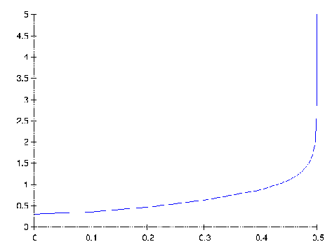
The values of the vevs $\langle W_{1}\rangle$ and $\langle W_{2}\rangle$ are the same since $\bar{u}_{i}=\bar{w}_{i}$ holds. Their values in the large $t$ limit are

	$\displaystyle\langle W_{1}\rangle\ =\ \langle W_{2}\rangle$	$\displaystyle=$	$\displaystyle-\frac{1}{4\varphi(b)(1+e^{\pi i\nu})t}\left[g^{\prime}(u_{0})G(u_{0})+g(u_{0})G^{\prime}(u_{0})\right]$		(2.39)
		$\displaystyle\to$	$\displaystyle 5.77\ .$

Note that these are finite even in the large $t$ limit, in contrast to ABJM theory and GT theory. The finiteness can be anticipated from the eigenvalue distribution. Recall that the large $t$ limit corresponds to the limit $\tau\to\nu$. The relation (2.34) implies that $a=1.19\times 10^{-2}$ in the limit which is small but finite. Then, the value of $b=a^{-1}$ is also finite. The following inequality

$$|\langle W_{1}\rangle|\ \leq\ \frac{1}{N_{1}}\sum_{i=1}^{N_{1}}e^{{\rm Re}(\bar{u}_{i})}\ \leq\ |b|$$

(2.40)

implies that $\langle W_{1}\rangle$ must be finite.

In fact, it turns out that all the observables derived from the resolvent $v(z)$ are finite in the large $t$ limit. To show this, consider a general situation in which $\rho(x;t)$ is a density function with a parameter $t$ whose support is an interval $I$. The expectation value of ${\cal O}(x)$ is defined as

$$\langle{\cal O}\rangle_{t}\ :=\ \int_{I}dx\,\rho(x;t){\cal O}(x).$$

(2.41)

Define a resolvent

$$\omega(z;t)\ :=\ t\int_{I}dx\,\rho(x;t)\frac{z+x}{z-x}.$$

(2.42)

The expectation value (2.41) can be written in terms of $\omega(z;t)$ as

$$\langle O\rangle_{t}\ =\ \frac{1}{2t}\int_{C}\frac{dz}{2\pi i}{\cal O}(z)\frac{\omega(z;t)}{z},$$

(2.43)

where $C$ is a contour in the $z$-plane encircling $I$ counterclockwise. Suppose that a function ${\cal F}(x)$ satisfies

$${\cal F}^{\prime}(x)\ =\ \frac{1}{x}{\cal O}(x).$$

(2.44)

Then, $\langle{\cal O}\rangle_{t}$ can be written as

$$\langle{\cal O}\rangle_{t}\ =\ -\frac{1}{2t}\int_{C}\frac{dz}{2\pi i}\frac{{\cal F}(z)}{z}\cdot z\omega^{\prime}(z;t).$$

(2.45)

This integral has a finite value in the limit $t\to\infty$ if $t^{-1}z\omega^{\prime}(z;t)$ has a finite limit at any points on the contour $C$.

In the case of the Chern-Simons-matter matrix models, the condition for the finiteness turns out to be

$$\lim_{t\to+\infty i}\left|t^{-1}\tilde{f}(u)\right|\ <\ \infty.\hskip 28.45274pt\left({\textstyle-\frac{1}{2}\leq u\leq+\frac{1}{2}}\right)$$

(2.46)

This can be shown to be the case numerically. Since this implies that the eigenvalue distribution of this matrix model has a finite limit, all the quantities calculated by using this eigenvalue distribution must be finite. Recall that the planar free energy is equal to $N^{2}$ times a quantity calculated by the eigenvalue distribution. Therefore, it scales as $N^{2}$, as for usual gauge theories.

If $n$ is large, then ${\rm Im}(\nu)$ becomes large. Then, since the pole of $t$ is located at the point $\tau=\nu$, the $q$-expansion of the theta functions can be used for the analysis of the large $t$ limit. The behavior of $t$ around $\tau=\nu$ turns out to be

$$t\ \sim\ \frac{r}{\tau-\nu},\hskip 28.45274ptr\ =\ \frac{2\,i}{\pi(e^{-\pi i\nu}-1)}.$$

(2.47)

This pole structure is qualitatively the same as (2.38) observed in the numerical result for $n=3$.

The vevs $\langle W_{\alpha}\rangle$ in the large $t$ limit are

$$\langle W_{1}\rangle\ =\ \langle W_{2}\rangle\ \to\ \frac{1}{1+e^{\pi i\nu}}.$$

(2.48)

This limiting value approaches 1 in the large $n$ limit. This can be anticipated from the saddle point equations (2.23)(2.24). As ${\rm Im}(\nu)$ becomes large, the attractive forces among the eigenvalues due to the second terms in the right-hand side of (2.23)(2.24) become strong. Then, the eigenvalue distribution shrinks to two points in the limit.

We observed in the previous subsection that the behavior of the vevs $\langle W_{\alpha}\rangle$ for the theories in CSM$(n\geq 3)$ is quite different from that of ABJM theory and GT theory. From the matrix model point of view, the difference comes from the fact that, in the former theories, the extent of the eigenvalue distributions are kept finite in the large ’t Hooft coupling limit, while in the latter theories, the eigenvalue distributions grow indefinitely. It is curious to know what happens if the eigenvalue distributions grow indefinitely in the former theories. It is not a strong coupling limit of the Chern-Simons-matter theories, but it could be realized by an analytic continuation of the parameters.

Since the branch points are constrained as (2.10)(2.12), an infinitely long distribution of the eigenvalues can be realized only when the parameter $a(=a_{1}=-a_{2})$ approaches zero. Small $a$ limit corresponds to a small $\tau$ limit. Due to the relation (2.34), they are related as

$$-\log a\ \sim\ \frac{\pi i}{2\tau}.$$

(2.49)

It turns out that it is not straightforward to take the limit $\tau\to 0$. Since the factor $(1+z(u_{\nu}))^{-1}$, which is the origin of the pole of $t$ at $\tau=\nu$, has in fact infinitely many poles on the $\tau$-plane for $n>2$. The positions of the poles are

$$\tau\ =\ \frac{\nu}{2l+1}+\frac{m}{2l+1}.\hskip 28.45274pt(l,m\in\mathbb{Z})$$

(2.50)

Therefore, the small $\tau$ limit taken along the imaginary axis, for example, is ill-defined.

One way to avoid these singularities is to take the following limit:

$$\tau\ =\ \varepsilon e^{i\theta},\hskip 28.45274pt\varepsilon\ \to\ 0$$

(2.51)

with a fixed $\theta$. It turns out that if $\theta$ is in the range

$$0\ <\ \cot\theta\ <\ \frac{1}{2\,{\rm Im}(\nu)},$$

(2.52)

then all the poles can be avoided. At the same time, the expansion of the theta functions, after the transformation $\tau\to-\frac{1}{\tau}$, behaves well.

The integral formula (2.19) gives the small $\tau$ behavior of $t$. The leading order term turns out to be

$$t\ \sim\ \frac{C}{\tau},\hskip 28.45274ptC\ :=\ \frac{1}{\sinh\left(\frac{\pi}{2}{\rm Im}(\nu)\right)}\sum_{n=1}^{\infty}\frac{(-i)^{n}}{n+\nu}.$$

(2.53)

Note that the sum in the coefficient $C$ for $n=3$ is finite:

$$\sum_{n=1}^{\infty}\frac{(-i)^{n}}{n+\nu}\ =\ -0.591-0.641\,i.$$

(2.54)

Then, an upper bound of the vevs $\langle W_{\alpha}\rangle$ is obtained as

$$|\langle W_{\alpha}\rangle|\ \leq\ |b|\ \lesssim\ \left|\exp\left(\frac{\pi i}{2C}t\right)\right|.$$

(2.55)

As in the cases for ABJM theory and GT theory, this upper bound is actually saturated. The formula (2.20) implies

$$\langle W_{\alpha}\rangle\ \sim\ \exp\left(\frac{\pi i}{2C}t\right)$$

(2.56)

for large $t$. This behavior is different from the Wilson loops in ABJM theory and GT theory.

The weak coupling behavior (2.29) indicates that there is another case $k_{1}=-k_{2}$ for which the analysis is rather simple. Assuming that $t$ takes a physical value, that is $t\in i\mathbb{R}$, the parameters $a_{1}$ and $a_{2}$ are related as

$$a_{1}\ =\ -a_{2}^{*}.$$

(2.57)

This is realized when the equalities $u_{i}=w_{i}^{*}$ are satisfied. This equality is compatible with the full saddle point equations (2.23)(2.24), and therefore, the relation (2.57) should hold beyond perturbation. Indeed, such eigenvalue distributions were discussed in [11][10].

When the relation (2.57) holds, the parameters $u_{0},u_{\infty}$, and $\tau$ in the resolvent $v(z)$ are related among them. In addition to the relation (2.31), one can show that $\tau$ is given as

$$\tau\ =\ 4i\,{\rm Im}(u_{0}).$$

(2.58)

Therefore, all the observables derived from the resolvent $v(z)$ are functions of $u_{0}$. Let $u_{0}$ be written as

$$u_{0}\ =\ u_{R}+\frac{1}{4}\tau,\hskip 28.45274ptu_{R}\ \in\ \mathbb{R},$$

(2.59)

the parameter $a_{1}$ is given as

$$a_{1}\ \sim\ 1-4e^{\frac{1}{2}\pi i\tau}e^{2\pi iu_{R}}$$

(2.60)

for large ${\rm Im}(\tau)$. The relation (2.29) for small $t$ implies that the physical curve $\gamma$, now on the $u_{0}$-plane, approaches the line

$${\rm Re}(u_{0})\ =\ \frac{1}{8}$$

(2.61)

in the small $t$ limit.

The large $t$ limit can be analyzed in the same way as in the case $k_{1}=k_{2}$. The plot of the curve $\gamma$ for $n=3$ turns out to be quite similar to figure 1. The curve $\gamma$ terminates on the imaginary axis of the $u_{0}$-plane. The intersection point is at

$$u_{0}\ =\ \frac{1}{4}\nu,$$

(2.62)

where $t$ diverges. The vevs $\langle W_{\alpha}\rangle$ are finite even in the large $t$ limit.

It was shown in [30] that the resolvent $v(z)$ satisfies the following vector equations:

	$\displaystyle(2\kappa_{1},0)$	$\displaystyle=$	$\displaystyle x_{1}v^{\prime}(x_{1}^{+})-x_{1}v^{\prime}(x_{1}^{-})M_{1},$		(4.1)
	$\displaystyle(0,2\kappa_{1})$	$\displaystyle=$	$\displaystyle x_{2}v^{\prime}(x_{2}^{+})-x_{2}v^{\prime}(x_{2}^{-})M_{2},$		(4.2)

where $x_{\alpha}\in I_{\alpha}$, and $x_{\alpha}^{+}$ ($x_{\alpha}^{-}$) is a point slightly above (below) $x_{\alpha}$. The matrices $M_{\alpha}$ are defined as

$$M_{1}\ :=\ \left[\begin{array}[]{cc}-1&0\\ n&1\end{array}\right],\hskip 28.45274ptM_{2}\ :=\ \left[\begin{array}[]{cc}1&n\\ 0&-1\end{array}\right].$$

(4.3)

In many cases, the left-hand sides of (4.1)(4.2) can be eliminated. This can be done by introducing $\omega(z)$ such that

$$zv^{\prime}(z)\ =\ c+\omega(z)$$

(4.4)

is satisfied, where the constant row vector $c$ satisfies

$$(2\kappa_{1},2\kappa_{2})\ =\ cA,\hskip 28.45274ptA\ :=\ \left[\begin{array}[]{cc}2&-n\\ -n&2\end{array}\right].$$

(4.5)

The solution exists as long as $n\neq 2$. Even in the case $n=2$, there exists a solution of this equation if and only if

$$\kappa_{1}+\kappa_{2}\ =\ 0$$

(4.6)

is satisfied. In the following, we assume that the equation (4.5) has a solution. Then, $\omega(z)$ satisfies

$$\omega(x_{\alpha}^{+})\ =\ \omega(x_{\alpha}^{-})M_{\alpha}.$$

(4.7)

It was shown in [30] that, for the case $n=2$, the vector equations (4.7) imply a simple scalar equation

$$\omega_{\psi_{2}}(x_{\alpha}^{+})\ =\ -\omega_{\psi_{2}}(x_{\alpha}^{-}),$$

(4.8)

where

$$\omega_{\psi}(z)\ :=\ \omega(z)\cdot\psi,\hskip 28.45274pt\psi_{2}\ :=\ \left[\begin{array}[]{c}1\\ -1\end{array}\right].$$

(4.9)

Therefore, $\omega_{\psi_{2}}(z)$ defines a two-sheeted covering of $\mathbb{C}$, that is, a torus.

For the case $n=1$, one can check that the following equations are satisfied:

$$\begin{array}[]{rclcrcl}\omega_{\psi_{1}}(x_{1}^{+})&=&\omega_{M_{1}\psi_{1}}(x_{1}^{-}),&&\omega_{\psi_{1}}(x_{2}^{+})&=&\omega_{\psi_{1}}(x_{2}^{-}),\\[5.69054pt] \omega_{M_{2}M_{1}\psi_{1}}(x_{1}^{+})&=&\omega_{M_{2}M_{1}\psi_{1}}(x_{1}^{-}),&&\omega_{M_{1}\psi_{1}}(x_{2}^{+})&=&\omega_{M_{2}M_{1}\psi_{1}}(x_{2}^{-}),\end{array}$$

(4.10)

where

$$\psi_{1}\ :=\ \left[\begin{array}[]{c}1\\ 0\end{array}\right].$$

(4.11)

The above equations imply that the three scalar functions $\omega_{\psi_{1}}(z),\omega_{M_{1}\psi_{1}}(z),\omega_{M_{2}M_{1}\psi}(z)$ define a three-sheeted covering of $\mathbb{C}$. After a compactification, the resulting curve is topologically a sphere. Note that these scalar functions are given in terms of the components of the resolvent $v(z)$ as

	$\displaystyle\omega_{\psi_{1}}(z)$	$\displaystyle=$	$\displaystyle zv_{1}^{\prime}(z)-c_{1},$		(4.12)
	$\displaystyle\omega_{M_{1}\psi_{1}}(z)$	$\displaystyle=$	$\displaystyle zv_{2}^{\prime}(z)-zv_{1}^{\prime}(z)+c_{1}-c_{2},$		(4.13)
	$\displaystyle\omega_{M_{2}M_{1}\psi_{1}}(z)$	$\displaystyle=$	$\displaystyle zv_{2}^{\prime}(z)-c_{2}.$		(4.14)

Similar spectral curves appeared in a different context [44][45].

References

- [1] O. Aharony, O. Bergman, D. L. Jafferis and J. Maldacena, “N=6 superconformal Chern-Simons-matter theories, M2-branes and their gravity duals,” JHEP 0810, 091 (2008) doi:10.1088/1126-6708/2008/10/091 [arXiv:0806.1218 [hep-th]].
- [2] J. M. Maldacena, “The Large N limit of superconformal field theories and supergravity,” Int. J. Theor. Phys. 38, 1113 (1999) [Adv. Theor. Math. Phys. 2, 231 (1998)] doi:10.1023/A:1026654312961 [hep-th/9711200].
- [3] D. Gaiotto and X. Yin, “Notes on superconformal Chern-Simons-Matter theories,” JHEP 0708, 056 (2007) doi:10.1088/1126-6708/2007/08/056 [arXiv:0704.3740 [hep-th]].
- [4] J. P. Gauntlett, G. W. Gibbons, G. Papadopoulos and P. K. Townsend, “Hyper-Kahler manifolds and multiply intersecting branes,” Nucl. Phys. B 500, 133 (1997) doi:10.1016/S0550-3213(97)00335-0 [hep-th/9702202].
- [5] J. Sparks, “Sasaki-Einstein Manifolds,” Surveys Diff. Geom. 16, 265 (2011) doi:10.4310/SDG.2011.v16.n1.a6 [arXiv:1004.2461 [math.DG]].
- [6] Y. Imamura and K. Kimura, “On the moduli space of elliptic Maxwell-Chern-Simons theories,” Prog. Theor. Phys. 120, 509 (2008) doi:10.1143/PTP.120.509 [arXiv:0806.3727 [hep-th]].
- [7] D. L. Jafferis and A. Tomasiello, “A Simple class of N=3 gauge/gravity duals,” JHEP 0810, 101 (2008) doi:10.1088/1126-6708/2008/10/101 [arXiv:0808.0864 [hep-th]].
- [8] P. M. Crichigno and D. Jain, “Non-toric Cones and Chern-Simons Quivers,” arXiv:1702.05486 [hep-th].
- [9] N. Drukker, M. Marino and P. Putrov, “From weak to strong coupling in ABJM theory,” Commun. Math. Phys. 306, 511 (2011) doi:10.1007/s00220-011-1253-6 [arXiv:1007.3837 [hep-th]].
- [10] C. P. Herzog, I. R. Klebanov, S. S. Pufu and T. Tesileanu, “Multi-Matrix Models and Tri-Sasaki Einstein Spaces,” Phys. Rev. D 83, 046001 (2011) doi:10.1103/PhysRevD.83.046001 [arXiv:1011.5487 [hep-th]].
- [11] T. Suyama, “On Large N Solution of ABJM Theory,” Nucl. Phys. B 834, 50 (2010) doi:10.1016/j.nuclphysb.2010.03.011 [arXiv:0912.1084 [hep-th]].
- [12] H. U. Yee, “AdS/CFT with Tri-Sasakian Manifolds,” Nucl. Phys. B 774, 232 (2007) doi:10.1016/j.nuclphysb.2007.03.031 [hep-th/0612002].
- [13] A. Kapustin, B. Willett and I. Yaakov, “Exact Results for Wilson Loops in Superconformal Chern-Simons Theories with Matter,” JHEP 1003, 089 (2010) doi:10.1007/JHEP03(2010)089 [arXiv:0909.4559 [hep-th]].
- [14] D. R. Gulotta, C. P. Herzog and S. S. Pufu, “From Necklace Quivers to the F-theorem, Operator Counting, and T(U(N)),” JHEP 1112, 077 (2011) doi:10.1007/JHEP12(2011)077 [arXiv:1105.2817 [hep-th]].
- [15] D. R. Gulotta, C. P. Herzog and S. S. Pufu, “Operator Counting and Eigenvalue Distributions for 3D Supersymmetric Gauge Theories,” JHEP 1111, 149 (2011) doi:10.1007/JHEP11(2011)149 [arXiv:1106.5484 [hep-th]].
- [16] P. M. Crichigno, C. P. Herzog and D. Jain, “Free Energy of Quiver Chern-Simons Theories,” JHEP 1303, 039 (2013) doi:10.1007/JHEP03(2013)039 [arXiv:1211.1388 [hep-th]].
- [17] D. Martelli and J. Sparks, “The large N limit of quiver matrix models and Sasaki-Einstein manifolds,” Phys. Rev. D 84, 046008 (2011) doi:10.1103/PhysRevD.84.046008 [arXiv:1102.5289 [hep-th]].
- [18] S. Cheon, H. Kim and N. Kim, “Calculating the partition function of N=2 Gauge theories on and AdS/CFT correspondence,” JHEP 1105, 134 (2011) doi:10.1007/JHEP05(2011)134 [arXiv:1102.5565 [hep-th]].
- [19] D. L. Jafferis, I. R. Klebanov, S. S. Pufu and B. R. Safdi, “Towards the F-Theorem: N=2 Field Theories on the Three-Sphere,” JHEP 1106, 102 (2011) doi:10.1007/JHEP06(2011)102 [arXiv:1103.1181 [hep-th]].
- [20] D. Martelli, A. Passias and J. Sparks, “The gravity dual of supersymmetric gauge theories on a squashed three-sphere,” Nucl. Phys. B 864, 840 (2012) doi:10.1016/j.nuclphysb.2012.07.019 [arXiv:1110.6400 [hep-th]].
- [21] A. Amariti, C. Klare and M. Siani, “The Large N Limit of Toric Chern-Simons Matter Theories and Their Duals,” JHEP 1210, 019 (2012) doi:10.1007/JHEP10(2012)019 [arXiv:1111.1723 [hep-th]].
- [22] D. Gang, C. Hwang, S. Kim and J. Park, “Tests of AdS4/CFT3 correspondence for chiral-like theory,” JHEP 1202, 079 (2012) doi:10.1007/JHEP02(2012)079 [arXiv:1111.4529 [hep-th]].
- [23] A. Amariti and S. Franco, “Free Energy vs Sasaki-Einstein Volume for Infinite Families of M2-Brane Theories,” JHEP 1209, 034 (2012) doi:10.1007/JHEP09(2012)034 [arXiv:1204.6040 [hep-th]].
- [24] S. Lee and D. Yokoyama, “Geometric free energy of toric AdS4/CFT3 models,” JHEP 1503, 103 (2015) doi:10.1007/JHEP03(2015)103 [arXiv:1412.8703 [hep-th]].
- [25] S. Gukov, C. Vafa and E. Witten, “CFT’s from Calabi-Yau four folds,” Nucl. Phys. B 584, 69 (2000) Erratum: [Nucl. Phys. B 608, 477 (2001)] doi:10.1016/S0550-3213(01)00289-9, 10.1016/S0550-3213(00)00373-4 [hep-th/9906070].
- [26] M. Billo, D. Fabbri, P. Fre, P. Merlatti and A. Zaffaroni, “Rings of short N=3 superfields in three-dimensions and M theory on AdS(4) x N**(0,1,0),” Class. Quant. Grav. 18, 1269 (2001) doi:10.1088/0264-9381/18/7/310 [hep-th/0005219].
- [27] D. Gaiotto and D. L. Jafferis, “Notes on adding D6 branes wrapping RP**3 in AdS(4) x CP**3,” JHEP 1211, 015 (2012) doi:10.1007/JHEP11(2012)015 [arXiv:0903.2175 [hep-th]].
- [28] S. Cheon, D. Gang, S. Kim and J. Park, “Refined test of AdS4/CFT3 correspondence for N=2,3 theories,” JHEP 1105, 027 (2011) doi:10.1007/JHEP05(2011)027 [arXiv:1102.4273 [hep-th]].
- [29] T. Nosaka and S. Yokoyama, “Complete factorization in minimal N=4 Chern-Simons-matter theory,” arXiv:1706.07234 [hep-th].
- [30] T. Suyama, “Notes on Planar Resolvents of Chern-Simons-matter Matrix Models,” JHEP 1611, 049 (2016) doi:10.1007/JHEP11(2016)049 [arXiv:1605.09110 [hep-th]].
- [31] N. Drukker, J. Plefka and D. Young, “Wilson loops in 3-dimensional N=6 supersymmetric Chern-Simons Theory and their string theory duals,” JHEP 0811, 019 (2008) doi:10.1088/1126-6708/2008/11/019 [arXiv:0809.2787 [hep-th]].
- [32] B. Chen and J. B. Wu, “Supersymmetric Wilson Loops in N=6 Super Chern-Simons-matter theory,” Nucl. Phys. B 825, 38 (2010) doi:10.1016/j.nuclphysb.2009.09.015 [arXiv:0809.2863 [hep-th]].
- [33] S. J. Rey, T. Suyama and S. Yamaguchi, “Wilson Loops in Superconformal Chern-Simons Theory and Fundamental Strings in Anti-de Sitter Supergravity Dual,” JHEP 0903, 127 (2009) doi:10.1088/1126-6708/2009/03/127 [arXiv:0809.3786 [hep-th]].
- [34] O. Aharony, O. Bergman and D. L. Jafferis, “Fractional M2-branes,” JHEP 0811, 043 (2008) doi:10.1088/1126-6708/2008/11/043 [arXiv:0807.4924 [hep-th]].
- [35] D. Gaiotto and A. Tomasiello, “The gauge dual of Romans mass,” JHEP 1001, 015 (2010) doi:10.1007/JHEP01(2010)015 [arXiv:0901.0969 [hep-th]].
- [36] M. Marino and P. Putrov, “Exact Results in ABJM Theory from Topological Strings,” JHEP 1006, 011 (2010) doi:10.1007/JHEP06(2010)011 [arXiv:0912.3074 [hep-th]].
- [37] T. Suyama, “On Large N Solution of Gaiotto-Tomasiello Theory,” JHEP 1010, 101 (2010) doi:10.1007/JHEP10(2010)101 [arXiv:1008.3950 [hep-th]].
- [38] T. Suyama, “A Systematic Study on Matrix Models for Chern-Simons-matter Theories,” Nucl. Phys. B 874, 528 (2013) doi:10.1016/j.nuclphysb.2013.06.008 [arXiv:1304.7831 [hep-th]].
- [39] A. Kapustin and N. Seiberg, “Coupling a QFT to a TQFT and Duality,” JHEP 1404, 001 (2014) doi:10.1007/JHEP04(2014)001 [arXiv:1401.0740 [hep-th]].
- [40] O. Aharony, D. Jafferis, A. Tomasiello and A. Zaffaroni, “Massive type IIA string theory cannot be strongly coupled,” JHEP 1011, 047 (2010) doi:10.1007/JHEP11(2010)047 [arXiv:1007.2451 [hep-th]].
- [41] T. Suyama, “Eigenvalue Distributions in Matrix Models for Chern-Simons-matter Theories,” Nucl. Phys. B 856, 497 (2012) doi:10.1016/j.nuclphysb.2011.11.013 [arXiv:1106.3147 [hep-th]].
- [42] R.W. Carter, “Lie Algebras of Finite and Affine Type,” Cambridge University Press.
- [43] H. Itoyama, T. Oota, T. Suyama and R. Yoshioka, “Cubic constraints for the resolvents of the ABJM matrix model and its cousins,” Int. J. Mod. Phys. A 32, no. 11, 1750056 (2017) doi:10.1142/S0217751X17500567 [arXiv:1609.03681 [hep-th]].
- [44] R. Dijkgraaf and C. Vafa, “On geometry and matrix models,” Nucl. Phys. B 644, 21 (2002) doi:10.1016/S0550-3213(02)00764-2 [hep-th/0207106].
- [45] H. Itoyama, K. Maruyoshi and T. Oota, “The Quiver Matrix Model and 2d-4d Conformal Connection,” Prog. Theor. Phys. 123, 957 (2010) doi:10.1143/PTP.123.957 [arXiv:0911.4244 [hep-th]].