Quantum steering with positive operator valued measures

Introduction. Ever since its first examination by Einstein, Podolsky, and Rosen (EPR) in 1935 [1], quantum nonlocality has been a puzzling phenomenon. In the EPR thought experiment, one observer, Alice, can perform a measurement on her half of an entangled pair to steer the other half (that belongs to a distant observer, Bob) to ensembles that conflict with the very intuition of classical locality [2]. This conflict was so profound that it prompted EPR to conclude that quantum theory was “incomplete” [1] and caused the longest debate in the history of quantum mechanics [3]. A more “complete” theory would be supplemented by hidden variables; however, the seminal work of Bell [4] demonstrated that no such theory, when constrained by locality, is capable of explaining all quantum mechanical predictions for bipartite systems. Nowadays, quantum nonlocality is perceived as one of the hallmarks of quantum theory that sets it apart from classical notions and underlies numerous quantum information applications [5].

Bell’s work defined the first class of quantum nonlocality, now known as Bell nonlocality [5]. Some 25 years later, Werner realised that Bell nonlocality and entanglement (nonseparability) were in fact two independent forms of quantum nonlocality [6]. In 2007, Wiseman, Jones and Doherty [7] recognised that the original idea of the EPR thought experiment is actually best captured by yet another form of quantum nonlocality – quantum steerability. Since then, quantum steerability has been successfully demonstrated experimentally in loophole-free tests [8, 9, 10]. It has been employed in a range of practical quantum information tasks, including quantum cryptography [11], randomness certification [12, 13], and self-testing [14, 15].

Among this surge of discoveries, a fundamental question remains: which bipartite states manifest quantum steerability? In fact, determining the steerability of a bipartite state when considering all possible measurements, i.e., positive operator valued measure (POVM) measurements, has been such a challenging task that it is unanswered for even the simplest case of two-qubit Werner states [16, Problem 39]. The problem remains open in spite of many significant advances towards understanding quantum steering under particular subsets of POVMs, e.g., with projection valued measure (PVM) measurements [7, 17, 18], with finite subsets of POVMs [19, 20], and with highly noisy POVMs or highly noisy states [21].

In this Letter, we are concerned with the problem of quantum steering with POVMs for bipartite systems of arbitrary (but finite) dimension. We demonstrate that for a given choice of local hidden state ensemble, the task of determining whether a quantum state is steerable can be considered as a nesting problem of two convex objects. As a consequence, we derive an inequality which allows a test of steerability for all measurements. Surprisingly, the inequality also reveals a fundamental aspect of quantum steering. Namely, in quantum steering, the choice of local hidden variable is no longer arbitrary as in Bell nonlocality, but can be limited to the set of Bob’s pure states. This in fact makes the study of quantum steering significantly simpler than its partner Bell nonlocality. In particular, one can strengthen the theorem (Lemma 1 of Ref. [7]) which limits the choice of local hidden state ensemble based on the symmetry of the state. As the first application, we then apply the inequality to study the steerability of the two-qubit Werner states. Contrary to the fact that general POVMs provide an advantage over PVMs in many situations [22, 23, 24], we provide strong numerical evidence that POVMs and PVMs are in fact equivalent for steering two-qubit Werner states.

Quantum steerability. Suppose Alice and Bob share a bipartite quantum state $\rho$ over the finite-dimensional Hilbert space $\mathcal{H}_{A}\otimes\mathcal{H}_{B}$. We use $\mathcal{A}^{H}$ (or $\mathcal{B}^{H}$) to denote the space of Hermitian operators over $\mathcal{H}_{A}$ (or $\mathcal{H}_{B}$). A POVM measurement with $n$ outcomes ($n$-POVM) $E$ implemented by Alice is an (ordered) collection of $n$ positive operators, $E=\{E_{i}\}_{i=1}^{n}$ with $E_{i}\in\mathcal{A}^{H}$, $E_{i}\geq 0$ and $\sum_{i=1}^{n}E_{i}=\mathbb{I}_{A}$, where $\mathbb{I}_{A}$ is the identity operator on $\mathcal{A}^{H}$. On performing the measurement, Alice steers Bob’s system to the steering ensemble $\{\operatorname{Tr}_{A}[\rho(E_{i}\otimes\mathbb{I}_{B})]\}_{i=1}^{n}$. However, despite the arbitrary choice of measurements, for certain bipartite states, the steering experiment can be locally simulated. More specifically, let $u$ be an ensemble (that is, a probability distribution) on the set of Bob’s pure states, denoted by $\mathcal{S}_{B}$. A state $\rho$ is then called $u$-unsteerable (always considered from Alice’s side) with respect to $n$-POVMs if, for any $n$-POVM $E$, Alice can find $n$ response functions $G_{i}$ (with $G_{i}(P)\geq 0$ and $\sum_{i=1}^{n}G_{i}(P)=1$ for all $P\in\mathcal{S}_{B}$) such that the steering ensemble can be simulated via a local hidden state model [7],

where the integral is taken over the Haar measure $\omega$ on Bob’s pure states $\mathcal{S}_{B}$. Equation (1) ensures that Bob, when performing state tomography conditioned on Alice’s outcomes, obtains the same result as if Alice were steering his system [7]. The ensemble $u$ is called a local hidden state (LHS) ensemble. In principle, the domain of the ensemble $u$ can be extended to mixed states. However, as a mixed state can be written as a convex combination of pure states, restricting the domain of $u$ to pure states causes no loss of generality. We say then that $\rho$ is unsteerable with $n$-POVMs if there exists $u$ such that $\rho$ is $u$-unsteerable with $n$-POVMs.

We note that this definition of quantum steering is slightly different from the original definition [7]. In the latter, the LHS ensemble is indexed by a local hidden variable. We will prove the two definitions are equivalent as parts of our results. Our seemingly minor simplification in fact has very important consequences, which will be discussed below.

The set of $n$-POVMs and its geometry. The key idea in our approach is that an $n$-POVM $E$ can be thought of as a point in the real vector space of composite operators $(\mathcal{A}^{H})^{\oplus n}=\oplus_{i=1}^{n}\mathcal{A}^{H}$. We therefore write $E=\oplus_{i=1}^{n}E_{i}$, which explicitly indicates that it is a composite operator in $(\mathcal{A}^{H})^{\oplus n}$ with components $E_{i}$ each bounded by $0\leq E_{i}\leq\mathbb{I}_{A}$. The space $(\mathcal{A}^{H})^{\oplus n}$ can be made Euclidean by defining an inner product $\left\langle X,Y\right\rangle=\sum_{i=1}^{n}\left\langle X_{i},Y_{i}\right\rangle$ for any composite operators $X$ and $Y$, where $\left\langle X_{i},Y_{i}\right\rangle$ denotes the Hilbert–Schmidt inner product of $\mathcal{A}^{H}$, $\left\langle X_{i},Y_{i}\right\rangle=\operatorname{Tr}(X^{\dagger}_{i}Y_{i})$. The set of $n$-POVMs is then a convex and compact subset of this space [25], which we denote by $\mathcal{M}^{n}$. Since $\sum_{i=1}^{n}E_{i}=\mathbb{I}_{A}$, $\mathcal{M}^{n}$ in fact belongs to the linear manifold $\mathcal{P}^{n}=\{X|\sum_{i=1}^{n}X_{i}=\mathbb{I}_{A}\}$.

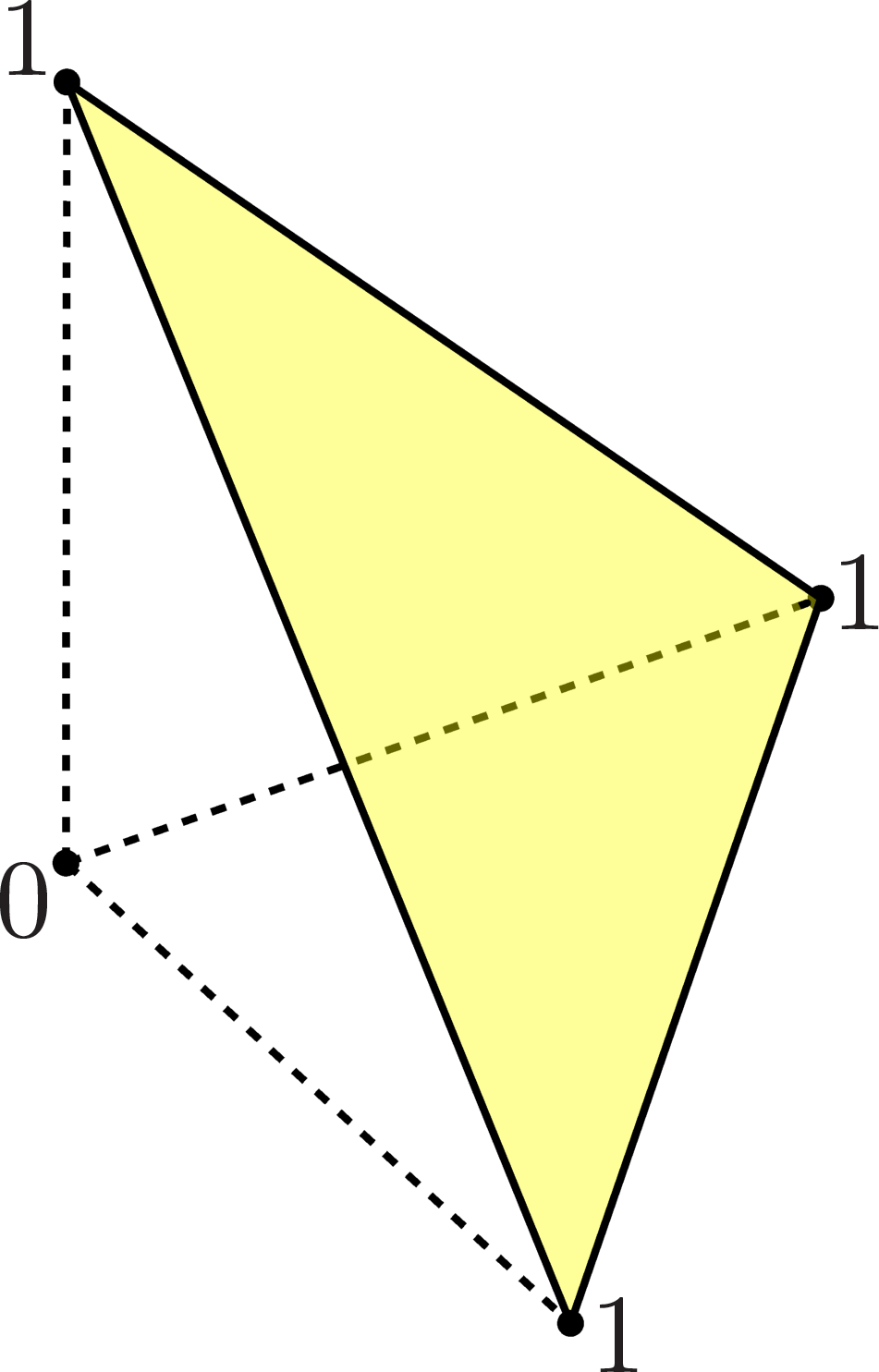
While the set of POVMs $\mathcal{M}^{n}$ is perhaps unfamiliar, it is similar to the classical probability simplexes. Figure 1 illustrates this similarity when $n=3$. The basis to construct a probability simplex is the probability range $[0,1]$. To obtain a probability simplex in $\mathbb{R}^{3}$, one aligns $3$ probability ranges $[0,1]$ along the $3$ axes and forms the triangle with vertices $(1,0,0)$, $(0,1,0)$, $(0,0,1)$. To construct the set of $3$-POVMs, the probability range $[0,1]$ is replaced by the set $0\leq X\leq\mathbb{I}_{A}$, which for qubits forms a double cone in $\mathcal{A}^{H}$ (illustrated in Figure 1) [26]. One then ‘aligns’ these $3$ sets $0\leq X\leq\mathbb{I}_{A}$ along the three orthogonal component spaces of $(\mathcal{A}^{H})^{\oplus 3}$. The set of $3$-POVMs is formed in between the points $(\mathbb{I}_{A},0,0)$, $(0,\mathbb{I}_{A},0)$, $(0,0,\mathbb{I}_{A})$. This analogy between a probability simplex and the set of $n$-POVMs applies in the same way for any $n$. There is, however, a crucial difference between classical probability simplexes and sets of POVMs: while $[0,1]$ is $1$-dimensional with $2$ extreme points $0$ and $1$, the set $0\leq X\leq\mathbb{I}_{A}$ is generally high-dimensional and with more extreme points other than $0$ and $\mathbb{I}_{A}$. As a result, the set of $n$-POVMs is also of high dimension and carries other extreme points apart from the special ones at the ‘corners’, which are of the form $\oplus_{i=1}^{n}\delta_{ik}\mathbb{I}_{A}$ with $k=1,2,\ldots n$.

The steering assemblage of $n$-POVMs. Now each POVM measurement $E$ performed on Alice’s side gives rise to a steering ensemble on Bob’s side, $\oplus_{i=1}^{n}\operatorname{Tr}_{A}[\rho(E_{i}\otimes\mathbb{I}_{B})]$. This is most easily implemented by the concept of a steering function $\rho^{A\to B}:\mathcal{A}^{H}\to\mathcal{B}^{H}$, which maps $X\in\mathcal{A}^{H}$ to $\operatorname{Tr}_{A}[\rho(X\otimes\mathbb{I}_{B})]\in\mathcal{B}^{H}$ [26]. This induces the map $(\rho^{A\to B})^{\oplus n}:(\mathcal{A}^{H})^{\oplus n}\to(\mathcal{B}^{H})^{\oplus n}$. For $X$ being an element or a subset of $\mathcal{A}^{H}$, we denote $X^{\prime}=\rho^{A\to B}(X)$. The same notation is used for composite vectors, namely, for $X$ being an element or a subset of $(\mathcal{A}^{H})^{\oplus n}$, $X^{\prime}=(\rho^{A\to B})^{\oplus n}(X)$.

Geometrically, the map $(\rho^{A\to B})^{\oplus n}$ maps a point in the set of POVMs $\mathcal{M}^{n}$ to a point in $(\mathcal{B}^{H})^{\oplus n}$. The set $(\mathcal{M}^{n})^{\prime}=(\rho^{A\to B})^{\oplus n}(\mathcal{M}^{n})$ is called the steering assemblage of $n$-POVMs. Being a linear image of $\mathcal{M}^{n}$, which is convex and compact [25], $(\mathcal{M}^{n})^{\prime}$ is also convex and compact. Moreover, since $\mathcal{M}^{n}$ belongs to $\mathcal{P}^{n}$, $(\mathcal{M}^{n})^{\prime}$ belongs to $(\mathcal{P}^{n})^{\prime}$.

The capacity of an ensemble of Bob’s pure states. For an ensemble $u$ of Bob’s pure states $\mathcal{S}_{B}$, the $n$-capacity $\mathcal{K}^{n}(u)$ is the set of $n$-component ensembles that it can simulate. That is to say, the capacity $\mathcal{K}^{n}(u)$ is a subset of $(\mathcal{B}^{H})^{\oplus n}$ consisting of composite operators $K=\oplus_{i=1}^{n}K_{i}$, each component being given by

with all possible choices of response functions $G_{i}$ that satisfy $G_{i}(P)\geq 0$, $\sum_{i=1}^{n}G_{i}(P)=1$. It is easy to show that the $n$-capacity $\mathcal{K}^{n}(u)$ is also a convex compact set, which has $n$ special extreme points of the form $\oplus_{i=1}^{n}\delta_{ik}\int\mathrm{d}\omega(P)u(P)P$ with $k=1,2,\ldots,n$.

Steerability as a nesting problem. With the above definitions, the following lemma is obvious.

We first consider the special extreme points of $\mathcal{M}^{n}$. It is easy to show that for their steering images to be in $\mathcal{K}^{n}(u)$, one has

which is referred to as the minimal requirement for $u$ ¹¹ 1 Since if $\int\mathrm{d}\omega(P)u(P)G_{i}(P)P=\mathbb{I}_{A}^{\prime}$ for some response function $G_{i}$, then by taking the trace of this equality, one obtains $\int\mathrm{d}\omega(P)u(P)G_{i}(P)=1$. Because $G_{i}(P)\geq 0$, this tells us that $G_{i}(P)=1$ almost everywhere with respect to the measure generated by $u$. This minimal requirement can also be obtained by summing both sides of equation (1) over $i$, bearing in mind the constraints $\sum_{i=1}^{n}E_{i}=\mathbb{I}_{A}$ and $\sum_{i=1}^{n}G_{i}(P)=1$. It can also be thought as the condition for $(\mathcal{M}^{1})^{\prime}\subseteq\mathcal{K}^{1}(u)$.

Once reformulated in terms of a nesting problem of convex objects (Lemma 1), one can apply nesting criteria to test steerability. The following lemma is such a nesting criterion based on a duality representation.

The idea behind this lemma is that if $\mathcal{X}$ contains $\mathcal{Y}$, then its projection onto any direction contains that of $\mathcal{Y}$ and vice versa (see Figure 2). A full proof is given in Appendix B.

To apply this lemma with $\mathcal{X}=\mathcal{K}^{n}(u)$, $\mathcal{Y}=(\mathcal{M}^{n})^{\prime}$, we need to solve two maximisation problems: $\max_{K\in\mathcal{K}^{n}(u)}\left\langle Z,K\right\rangle$ and $\max_{E\in\mathcal{M}^{n}}\left\langle Z,E^{\prime}\right\rangle$ for a given composite operator $Z$ in $(\mathcal{B}^{H})^{\oplus n}$. While the latter is a semidefinite program, the former is a linear constrained maximisation, which can be solved explicitly (see Appendix C for the details):

From Lemma 1 and Lemma 2, the following theorem immediately follows.

Inequality (5) is the main result in this Letter: it is valid for systems of arbitrary dimension and POVMs of arbitrary number of outcomes. We now discuss some of its important consequences; details of proofs and further discussions are given in Appendix D.

Had one started with the original definition of quantum steering with an “indexed LHS ensemble”, that is, an LHS ensemble indexed by some hidden variable, one would arrive at a similar inequality as (5). In that case, the integration is taken over the hidden variable instead (see Appendix D). However, one can rewrite it as an integral over the push-forward measure over Bob’s pure states $\mathcal{S}_{B}$ [28]. This implies that it is only the push-forward measure on $\mathcal{S}_{B}$ that really determines the capacity of an LHS ensemble. Two indexed LHS ensembles generating the same measure on Bob’s pure states would have the same capacity. In other words, our definition of quantum steering where the local hidden variable is omitted is equivalent to the original definition of quantum steering (Corollary 1, Appendix D). Having eliminated the arbitrary choice of local hidden variable in quantum steering, the symmetry of the state directly has a stronger implication on the symmetry of LHS ensembles (see Theorem 2). In fact, it is this stronger implication of symmetry that actually renders many unsolvable problems in Bell nonlocality solvable in the context of quantum steering [7].

More specifically, the state $\rho$ is said to have $(\mathcal{G},U,V)$-symmetry with $\mathcal{G}$ being a group and $U$ and $V$ being its two representations on $\mathcal{H}_{A}$ and $\mathcal{H}_{B}$, respectively, if $\rho=U^{\dagger}(g)\otimes V^{\dagger}(g)\rho U(g)\otimes V(g)$ for all $g\in\mathcal{G}$. The action $V$ of $\mathcal{G}$ on Bob’s pure states $\mathcal{S}_{B}$ generates an action $R_{V}$ on the space of distributions on $\mathcal{S}_{B}$ defined by $[R_{V}(g)u](P)=u[V^{\dagger}(g)PV(g)]$. We then have a strengthened form of Lemma 1 of Ref. [7] on the symmetry of LHS ensemble.

This theorem is applicable as well when measurements are restricted to PVMs. To understand the difference with Lemma 1 of Ref. [7], we consider the example where $\mathcal{G}$ acts transitively on Bob’s pure states $\mathcal{S}_{B}$ (i.e., a single orbit covers all of $\mathcal{S}_{B}$). If $\rho$ is unsteerable, Lemma 1 of Ref. [7] then states the existence of an indexed LHS ensemble, on which $\mathcal{G}$ acts covariantly on the indices and the states. However, due to the arbitrariness in choice of the local hidden variable, there exist in fact infinitely many different $\mathcal{G}$-covariant indexed LHS ensembles (see Appendix D). One then could not single out an unique choice of LHS ensemble. On the other hand, under the same conditions, Theorem 2 implies that the state is unsteerable with the unique uniform distribution on Bob’s pure states as an LHS ensemble.

Beyond revealing very general aspects of quantum steering, Theorem 1 can also be used to test steerability in practice. The most difficult part is to determine the existence of a LHS ensemble $u$. Even when measurements are limited to PVMs, the question is so far solved only for highly symmetric states, e.g., the Werner state [7] and the two-qubit $T$-state (mixtures of Bell states) [17, 18]. The implication of our approach on this problem will be discussed elsewhere. However, as we mentioned, even when $u$ is known, the problem of determining steerability with POVMs is still open [16, Problem 39]. It is this latter problem that we are concerned with in the following. We will show that Theorem 1 can provide a strong numerical evidence for steering with POVMs with a given identified candidate for the LHS ensemble.

The gap function. We first note that for a LHS ensemble $u$ satisfying the minimal requirement (3), the inequality (5) is invariant with respect to the transformation $\oplus_{i=1}^{n}Z_{i}\to\frac{1}{\sqrt{D}}\oplus_{i=1}^{n}(Z_{i}-C)$, where $C=\frac{1}{n}\sum_{i=1}^{n}Z_{i}$ and $D=\sum_{i=1}^{n}\left\langle Z_{i}-C,Z_{i}-C\right\rangle$. We can therefore restrict $Z$ to the set of those satisfying $\sum_{i=1}^{n}Z_{i}=0$ and $\sum_{i=1}^{n}\left\langle Z_{i},Z_{i}\right\rangle=1$, denoted by $\mathcal{C}^{n}$. For clarity, we introduce the gap function $\Delta[(\mathcal{M}^{n})^{\prime},\mathcal{K}^{n}(u)]$, defined to be

The gap function characterises the gap between the boundary of $(\mathcal{M}^{n})^{\prime}$ and that of $\mathcal{K}^{n}(u)$ from inside. The state $\rho$ is $u$-unsteerable with $n$-POVMs if and only if $\Delta[(\mathcal{M}^{n})^{\prime},\mathcal{K}^{n}(u)]\geq 0$.

Restriction to rank-$1$ POVMs. As all POVMs can be post-processed from those of rank-$1$, to test quantum steerability we can concentrate on the latter [29]. To this end, we define $\mathcal{\widetilde{\mathcal{M}}}^{n}=\{\oplus_{i=1}^{n}\alpha_{i}P_{i}\}$ where $P_{i}$ are (not necessarily independent) rank-$1$ projections and $0\leq\alpha_{i}\leq 1$ such that $\sum_{i=1}^{n}\alpha_{i}P_{i}=\mathbb{I}_{A}$. To test the steerability with $\mathcal{M}^{n}$, we therefore only need to calculate $\Delta[(\widetilde{\mathcal{M}}^{n})^{\prime},\mathcal{K}^{n}(u)]$.

Steerability of two-qubit Werner states with POVMs. Consider the two-qubit Werner state,

which is a mixing between the singlet Bell state $\left|\psi^{-}\right\rangle=\frac{1}{\sqrt{2}}(\left|01\right\rangle-\left|10\right\rangle)$ and the maximally mixed state with mixing parameter $p$ ($0\leq p\leq 1$). When restricted to PVMs, by explicitly constructing the response functions, it was shown that the Werner state is unsteerable for the mixing probabilities $p\leq\frac{1}{2}$ [7]. By adapting Barrett’s model [29] of local hidden variables, it was further possible to show that Werner states are unsteerable with POVMs when $p\leq\frac{5}{12}$ [21]. We are to study the conjecture [30]:

Although further analyses restricted to finite subsets of POVMs [19, 20] or POVMs with special symmetry [30] support unsteerability of the Werner state for $\frac{5}{12}\leq p\leq\frac{1}{2}$ [31, 30], there has not been a concrete evidence when one considers all POVMs. For $n=1$, the conjecture is obvious. For $n=2$, it has been proven by demonstrating the equivalence to steering with PVMs [26]. The proof for $n=3$ is also known [30]. Finally, it is known that it is sufficient to consider the conjecture for $n=4$ [32, 30]. Here, by computing the corresponding gap function for the Werner state, we provide strong numerical evidence for Conjecture 1 for $n=4$.

It is easy to see that the Werner state has $\operatorname{U}(2)$ symmetry as defined above. Moreover, since the action is transitive on Bob’s Bloch sphere, by Theorem 2, the candidate for the LHS ensemble can be limited to the uniform distribution, $u=1$. To simplify the notation, from now on we simply use $\Delta$ to denote the gap function without specifying the set of measurements and the capacity, which can be understood from the context. The computation of the gap function $\Delta$ generally requires global minimisation over $Z$, which is carried out by the standard (non-deterministic) simulated annealing algorithm (see Appendix E for details).

In Figure 3, we present values of $\Delta$ found for the mixing probability $p\approx\frac{1}{2}$. For comparison, we also present the numerical results of $\Delta$ when the measurements are limited to PVMs, which are in very good agreement with the analytical calculation (see Appendix F). For $p>\frac{1}{2}$, one observes that the gap function $\Delta$ for rank-$1$ $4$-POVMs is negative and coincides with the gap function for PVMs. For all $p\leq\frac{1}{2}-10^{-3}$, the best obtained values for $\Delta$ are less than $10^{-10}$ but persistently non-negative. The fact that the gap function tends to vanish for $p\leq\frac{1}{2}$ instead of attending finite positive values seems to be because of the high dimensionality of POVMs ²² 2 The effect of dimensionality can be understood directly from Figure 2. On the plane, the gap between the boundaries of the two objects is positive. However when imbedded in the 3D space, the gap will be zero in direction that is perpendicular to plane that contains the two objects. The presented results therefore support conjecture 1. Unfortunately, within this work, the ambiguity region of $\frac{1}{2}-10^{-3}\leq p\leq\frac{1}{2}$ cannot be resolved due to limits of numerical accuracy (see Appendix E).

Conclusion. Our work simplifies the definition of quantum steering, where we show that the local hidden variable indexing LHS ensemble can be omitted. As a direct consequence, a stronger theorem on the symmetry of the LHS ensemble is derived. We have thereby opened a general approach to studying quantum steerability with POVMs. Further works to strengthen the numerical evidence for the unsteerability of the Werner state at $p=\frac{1}{2}$ and testing steerability with POVMs of arbitrary two-qubit states are underway. Moreover, although the current illustrative applications are based on two qubits, our approach is not limited by the dimensionality of the systems. It is hoped that systematic tests for steering with POVMs (particularly for high dimensional systems) will give a complete answer to the fundamental question of the equivalence between POVMs and PVMs for steerability. Beyond quantum steering, we leave open the question of whether this approach can be extended to characterise Bell nonlocality with POVMs.

References

- [1] A. Einstein, B. Podolsky, and N. Rosen, “Can quantum-mechanical description of physical reality be considered complete?” Phys. Rev. 47, 777–780 (1935).
- [2] E. Schrödinger, “Probability relations between separated systems,” Math. Proc. Camb. Philos. Soc. 32, 446–452 (1936).
- [3] J. S. Bell, Speakable and unspeakable in quantum mechanics: Collected papers on quantum philosophy (Cambridge University Press, Cambridge, 2004).
- [4] J. Bell, “On the Einstein Podolsky Rosen paradox,” Physics 1, 195–200 (1964).
- [5] N. Brunner, D. Cavalcanti, S. Pironio, V. Scarani, and S. Wehner, “Bell nonlocality,” Rev. Mod. Phys. 86, 419–478 (2014).
- [6] R. F. Werner, “Quantum states with Einstein-Podolsky-Rosen correlations admitting a hidden-variable model,” Phys. Rev. A 40, 4277 (1989).
- [7] H. M. Wiseman, S. J. Jones, and A. C. Doherty, “Steering, entanglement, nonlocality, and the Einstein-Podolsky-Rosen paradox,” Phys. Rev. Lett. 98, 140402 (2007).
- [8] A. J. Bennet, D. A. Evans, D. J. Saunders, C. Branciard, E. G. Cavalcanti, H. M. Wiseman, and G. J. Pryde, “Arbitrarily loss-tolerant Einstein-Podolsky-Rosen steering allowing a demonstration over 1 km of optical fiber with no detection loophole,” Phys. Rev. X 2, 031003 (2012).
- [9] D. H. Smith, G. Gillett, M. P. de Almeida, C. Branciard, A. Fedrizzi, T. J. Weinhold, A. Lita, B. Calkins, T. Gerrits, H. M. Wiseman, S. W. Nam, and A. C. White, “Conclusive quantum steering with superconducting transition-edge sensors,” Nat. Commun. 3 (2012).
- [10] B. Wittmann, S. Ramelow, F. Steinlechner, N. K. Langford, N. Brunner, H. M. Wiseman, R. Ursin, and A. Zeilinger, “Loophole-free Einstein-Podolsky-Rosen experiment via quantum steering,” New J. Phys. 14 (2012).
- [11] C. Branciard, E. G. Cavalcanti, S. P. Walborn, V. Scarani, and H. M. Wiseman, “One-sided device-independent quantum key distribution: Security, feasibility, and the connection with steering,” Phys. Rev. A 85, 010301 (2012).
- [12] Y. Z. Law, L. P. Thinh, J.-D. Bancal, and V. Scarani, “Quantum randomness extraction for various levels of characterization of the devices,” Journal of Physics A: Mathematical and Theoretical 47, 424028 (2014).
- [13] E. Passaro, D. Cavalcanti, P. Skrzypczyk, and A. Acín, “Optimal randomness certification in the quantum steering and prepare-and-measure scenarios,” New Journal of Physics 17, 113010 (2015).
- [14] I. Šupić and M. J. Hoban, “Self-testing through EPR-steering,” New J. Phys. 18 (2016).
- [15] A. Gheorghiu, P. Wallden, and E. Kashefi, “Rigidity of quantum steering and one-sided device-independent verifiable quantum computation,” New J. Phys. 19 (2017).
- [16] “Open quantum problems,” https://oqp.iqoqi.univie.ac.at/ (2017).
- [17] S. Jevtic, M. J. W. Hall, M. R. Anderson, M. Zwierz, and H. M. Wiseman, “Einstein–Podolsky–Rosen steering and the steering ellipsoid,” J. Opt. Soc. Am. B 32, A40–A49 (2015).
- [18] H. C. Nguyen and T. Vu, “Necessary and sufficient condition for steerability of two-qubit states by the geometry of steering outcomes,” Europhys. Lett. 115, 10003 (2016a).
- [19] D. Cavalcanti, L. Guerini, R. Rabelo, and P. Skrzypczyk, “General method for constructing local hidden variable models for entangled quantum states,” Phys. Rev. Lett. 117, 190401 (2016).
- [20] F. Hirsch, M. T. Quintino, T. Vértesi, M. F. Pusey, and N. Brunner, “Algorithmic construction of local hidden variable models for entangled quantum states,” Phys. Rev. Lett. 117, 190402 (2016).
- [21] M. T. Quintino, T. Vértesi, D. Cavalcanti, R. Augusiak, M. Demianowicz, A. Acín, and N. Brunner, “Inequivalence of entanglement, steering, and bell nonlocality for general measurements,” Phys. Rev. A 92, 032107 (2015).
- [22] T. Vértesi and E. Bene, “Two-qubit Bell inequality for which positive operator-valued measurements are relevant,” Phys. Rev. A 82, 062115 (2010).
- [23] F. Hirsch, M. T. Quintino, J. Bowles, and N. Brunner, “Genuine hidden quantum nonlocality,” Phys. Rev. Lett. 111, 160402 (2013).
- [24] A. Acín, S. Pironio, T. Vértesi, and P. Wittek, “Optimal randomness certification from one entangled bit,” Phys. Rev. A 93, 040102 (2016).
- [25] G. Chiribella, G. M. D’Ariano, and D. Schlingemann, “How continuous quantum measurements in finite dimensions are actually discrete,” Phys. Rev. Lett. 98, 190403 (2007).
- [26] H. C. Nguyen and T. Vu, “Nonseparability and steerability of two-qubit states from the geometry of steering outcomes,” Phys. Rev. A 94, 012114 (2016b).
- [27] Since if for some response function , then by taking the trace of this equality, one obtains . Because , this tells us that almost everywhere with respect to the measure generated by . This minimal requirement can also be obtained by summing both sides of equation (1) over , bearing in mind the constraints and . It can also be thought as the condition for .
- [28] Vladimir I. Bogachev, Measure theory (Springer-Verlag, Berlin Heidelberg, 2007).
- [29] J. Barrett, “Nonsequential positive-operator-valued measurements on entangled mixed states do not always violate a Bell inequality,” Phys. Rev. A 65, 042302 (2002).
- [30] R. F. Werner, “Steering, or maybe why Einstein did not go all the way to Bell’s argument,” J. Phys. A: Math. Theor. 47, 424008 (2014).
- [31] J. Bavaresco, M. T. Quintino, L. Guerini, T. O. Maciel, D. Cavalcanti, and M. T. Cunha, “Most incompatible measurements for robust steering tests,” arXiv:1704.02994 [quant-ph] (2017).
- [32] G. M. D’Ariano, P. L. Presti, and P. Perinotti, “Classical randomness in quantum measurements,” Journal of Physics A: Mathematical and General 38, 5979 (2005).
- [33] The effect of dimensionality can be understood directly from Figure 2. On the plane, the gap between the boundaries of the two objects is positive. However when imbedded in the 3D space, the gap will be zero in direction that is perpendicular to plane that contains the two objects.
- [34] S.-T. Hu, Elements of real analysis (Holden-Day, Inc., San Francisco, 1967).
- [35] J. B. Conway, A Course in Functional Analysis (Springer, 1990).
- [36] R. T. Rockafellar, Convex analysis (Princeton University Press, Princeton, 2015).
- [37] W. H. Press, B. P. Flannery, S. A. Teukolsky, W. T. Vetterling, and B. P. Flannery, Numerical recipes, 3rd ed. (Cambridge University Press, Cambridge, 2007).
- [38] V. Granville, M. Krivanek, and J. P. Rasson, “Simulated annealing: a proof of convergence,” IEEE Trans. Pattern Anal. Mach. Intell. 16, 652–656 (1994).
- [39] Gaël Guennebaud, Benoît Jacob, et al., “Eigen v3,” http://eigen.tuxfamily.org (2010).
- [40] R. H. Swendsen and J.-S. Wang, “Replica Monte Carlo simulation of spin-glasses,” Phys. Rev. Lett. 57, 2607 (1986).
- [41] J. S. Arora, O. A. Elwakeil, A. I. Chahande, and C. C. Hsieh, “Global optimization methods for engineering applications: A review,” Struct. Optim. 9, 137–159 (1995).