Lyapunov Exponent Evaluation of the CBC Mode of Operation

Abdessalem Abidi Christophe Guyeux Jacques Demerjian Affiliation: Belagacem Bouallègue, and Mohsen Machhout

Abstract

The Cipher Block Chaining (CBC) mode of encryption was invented in 1976, and it is currently one of the most commonly used mode. In our previous research works, we have proven that the CBC mode of operation exhibits, under some conditions, a chaotic behavior. The dynamics of this mode has been deeply investigated later, both qualitatively and quantitatively, using the rigorous mathematical topology field of research. In this article, which is an extension of our previous work, we intend to compute a new important quantitative property concerning our chaotic CBC mode of operation, which is the Lyapunov exponent.

1 Introduction

Blocks ciphers, like Data Encryption Standard (DES) or Advanced Encryption Standard (AES), have a very simple principle: they do not treat the original text bit by bit but they manipulate blocks of text. More precisely, the plaintext is broken into blocks of $\mathsf{N}$ bits. For each one, the encryption algorithm is applied to obtain an encrypted block that has the same size. Then, we put together all of these blocks, which are separately encrypted, to obtain the full encrypted message. For decryption, we proceed in the same way, but now starting from the ciphertext, in order to obtain the original one employing the decryption algorithm in place of the encryption function. So it is not sufficient to put anyhow a block cipher algorithm in a program. We can, instead, use these algorithms in various ways according to their specific needs. These ways are called block cipher modes of operation. Indeed, there are several modes and each one of them differs from others by its own characteristics, in addition to its specific security properties. In this article, we are only interested in the Cipher Block Chaining mode and we will quantify its chaotic behavior thanks to the Lyapunov exponent. To do so, we first show that such mode of operations can be considered as dynamical systems.

Indeed, some dynamical systems are very sensitive to small changes in their initial condition. Both constants of sensitivity to initial conditions and of expansivity illustrate that [1, 2]. However, these variations can quickly take enormous proportions, grow exponentially, and none of these constants can measure such a behavior. Alexander Lyapunov has examined this phenomenon and introduced an exponent that measures the rate at which these small variations can grow.

Definition 1

Let $f:\mathds{R}\longrightarrow\mathds{R}$ . The Lyapunov exponent of the system defined by $x^{0}\in\mathds{R}$ and $x^{n+1}=f(x^{n})$ is:

\displaystyle{\lambda(x_{0})=\lim_{n\to+\infty}\dfrac{1}{n}\sum_{i=1}^{n}\ln\left|~f^{\prime}\left(x^{i-1}\right)\right|}.

_□

Consider a dynamical system with an infinitesimal error on the initial condition $x_{0}$ . When the Lyapunov exponent is positive, this error will increase (situation of chaos), whereas it will decrease if $\lambda(x_{0})\leqslant 0$ .

Example 1

The Lyapunov exponent of the logistic map $x^{0}\in[0,1]$ , $x^{n+1}=\mu x^{n}(1-x^{n})$ [3] becomes positive for $\mu>3,54$ , but it is always smaller than 1. The tent map [4, 5] and the doubling map of the circle [6], two other well-known chaotic dynamical systems, have a Lyapunov exponent equal to $\ln(2)$ . _□

Sometimes, instead of trying to prove directly the properties on the system itself, it is preferable to reduce the initial problem to another whose characteristics are known or seem to be accessible. Such a reduction tool is called, in the mathematical theory of chaos, the semi-conjugacy.

Definition 2

The discrete dynamical system $(\mathcal{X},f)$ is topologically semi-conjugate to the system $(\mathcal{Y},g)$ if it exists a function $\varphi:\mathcal{X}\longrightarrow\mathcal{Y}$ , both continuous and onto, such that:

\varphi\circ f=g\circ\varphi,

that is, which makes commutative the following diagram [7].

\begin{CD}\mathcal{X}@>{f}>{}>\mathcal{X}\\ @V{\varphi}V{}V@V{}V{\varphi}V\\ \mathcal{Y}@>{}>{g}>\mathcal{Y}\end{CD}

In this case, the system $(\mathcal{Y},g)$ is called a factor of the system $(\mathcal{X},f)$ . _□

Various dynamical behaviors are inherited by systems factors [7]. They are summarized in the following proposition:

Proposition 1

Let $(\mathcal{Y},g)$ a factor of the system $(\mathcal{X},f)$ . Then:

1.

for all $j\leqslant k$ , $p\in Per_{k}(f)\Longrightarrow\varphi(p)\in Per_{j}(g)$ , where $Per_{n}(h)$ stands for the set of points of period $n$ for the iteration function $h$ .
2.

$(\mathcal{X},f)$ regular $\Longrightarrow$ $(\mathcal{Y},g)$ regular,
3.

$(\mathcal{X},f)$ transitive $\Longrightarrow$ $(\mathcal{Y},g)$ transitive.

So if $(\mathcal{X},f)$ is chaotic as defined by Devaney, then $(\mathcal{Y},g)$ is chaotic too. _□

Having these materials in mind, it is now possible to measure the Lyapunov exponent of some CBC mode of operations. Do do so, we will follow the canvas described hereafter. In Section 2, some basic reminders are given. The semiconjugacy allowing the exponent evaluation is described in Section 3. In the next one, the consequences of such a semi-conjugacy are outlined, and the exponent is computed. This article ends by a conclusion section where our contribution is summarized and intended future work is outlined.

2 Basic Recalls

2.1 The Cipher Block Chaining (CBC) mode

The CBC block cipher mode of operation presents a very popular way of encryption that is used in numerous applications, despite the fact that encryption in this mode can be performed only using one thread. Cipher block chaining is a block cipher mode that provides confidentiality but not message integrity in cryptography. The operating principle of this mode is to add XOR each subsequent plain-text block to a cipher-text one that was previously received, see Figure 1. Each subsequent cipher-text block depends on the previous one. Finally, the first plain-text block is added XOR to a random Initialization Vector (commonly referred to as IV). This vector has the same size as all plain-text blocks.

To decrypt cipher-text blocks, one should add XOR output data from decryption algorithm to previous cipher-text blocks. The receiver knows all cipher-text blocks just after obtaining encoded the message, thus he can decrypt the message using many threads simultaneously. If one bit of a plain-text message is damaged (for instance, because of some earlier transmission error), all subsequent cipher-text blocks will be damaged and it will be never possible to decrypt the cipher-text received from this plain-text. As opposed to that, if one cipher-text bit is damaged, only two received plain-text blocks will be damaged.

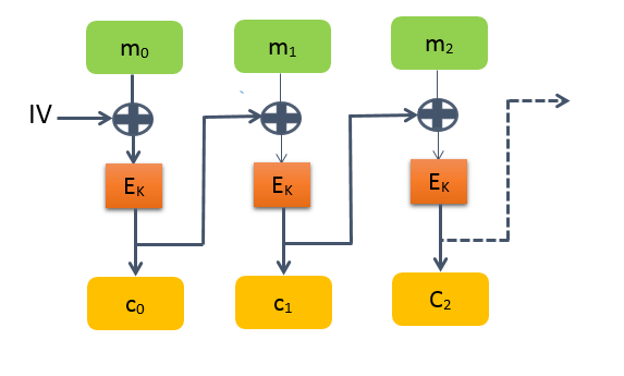
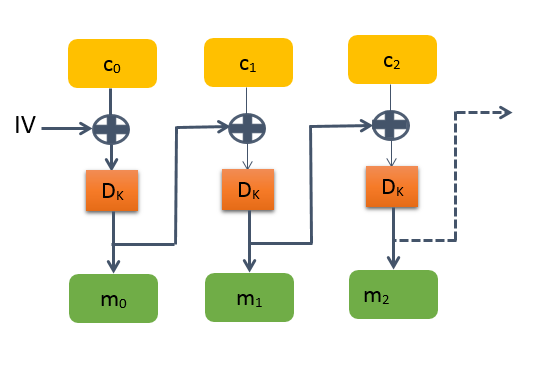
Refer to caption — (a) CBC encryption mode

Finally, note that a message that is to be encrypted using the CBC mode, should be extended until being as long as a multiple of a single block length.

2.2 Modeling the CBC mode as a dynamical system

Our modeling follows a same canvas than what has be done for hash functions [8, 1] or pseudo-random number generation [9]. Let us consider the CBC mode of operation with a keyed encryption function $\varepsilon_{k}:\mathds{B}^{\mathsf{N}}\rightarrow\mathds{B}^{\mathsf{N}}$ depending on a secret key $k$ , where $\mathsf{N}$ is the size for the block cipher, and $\mathcal{D}_{k}:\mathds{B}^{\mathsf{N}}\rightarrow\mathds{B}^{\mathsf{N}}$ is the associated decryption function, which is such that $\forall k,\varepsilon_{k}\circ\mathcal{D}_{k}$ is the identity function. We define the Cartesian product $\mathcal{X}=\mathds{B}^{\mathsf{N}}\times\mathcal{S}_{\mathsf{N}}$ , where:

•

$\mathds{B}=\{0,1\}$ is the set of Boolean values,
•

$\mathcal{S}_{\mathsf{N}}=\llbracket 0,2^{\mathsf{N}}-1\rrbracket^{\mathds{N}}$ , the set of infinite sequences of natural integers bounded by $2^{\mathsf{N}}-1$ , or the set of infinite $\mathsf{N}$ -bits block messages,

in such a way that $\mathcal{X}_{\mathsf{N}}$ is constituted by couples of internal states of the mode of operation together with sequences of block messages. Let us consider the initial function:

\begin{array}[]{cccc}i:&\mathcal{S}_{\mathsf{N}}&\longrightarrow&\llbracket 0,2^{\mathsf{N}}-1\rrbracket\\ &(m^{i})_{i\in\mathds{N}}&\longmapsto&m^{0}\end{array}

that returns the first block of a (infinite) message, and the shift function:

\begin{array}[]{cccc}\sigma:&\mathcal{S}_{\mathsf{N}}&\longrightarrow&\mathcal{S}_{\mathsf{N}}\\ &(m^{0},m^{1},m^{2},...)&\longmapsto&(m^{1},m^{2},m^{3},...)\end{array}

which removes the first block of a message. Let $m_{j}$ be the $j$ -th bit of integer, or block message, $m\in\llbracket 0,2^{\mathsf{N}}-1\rrbracket$ , expressed in the binary numeral system, and when counting from the left. We define:

\begin{array}[]{cccc}F_{f}:&\mathds{B}^{\mathsf{N}}\times\llbracket 0,2^{\mathsf{N}}-1\rrbracket&\longrightarrow&\mathds{B}^{\mathsf{N}}\\ &(x,m)&\longmapsto&\left(x_{j}m_{j}+f(x)_{j}\overline{m_{j}}\right)_{j=1..\mathsf{N}}\end{array}

This function returns the inputted binary vector $x$ , whose $m_{j}$ -th components $x_{m_{j}}$ have been replaced by $f(x)_{m_{j}}$ , for all $j=1..\mathsf{N}$ such that $m_{j}=0$ . In case where $f$ is the vectorial negation, this function will correspond to one XOR between the clair text and the previous encrypted state.

Denote by $f_{0}$ the vectorial negation. So the CBC mode of operation can be rewritten n a condensed way, as follows.

\left\{\begin{array}[]{ll}X^{0}=&(IV,m)\\ X^{n+1}=&\left(\mathcal{E}_{k}\circ F_{f_{0}}\left(i(X_{1}^{n}),X_{2}^{n}\right),\sigma(X_{1}^{n})\right)\end{array}\right.

(1)

For any given $g:\llbracket 0,2^{\mathsf{N}}-1\rrbracket\times\mathds{B}^{\mathsf{N}}\longrightarrow\mathds{B}^{\mathsf{N}}$ , we denote $G_{g}(X)=\left(g(i(X_{1}),X_{2});\sigma(X_{1})\right)$ (when $g=\mathcal{E}_{k}\circ F_{f_{0}}$ , we obtain one cypher block of the CBC, as depicted in Figure 1). So the recurrent relation of Eq.(1) can be rewritten in a condensed way, as follows.

X^{n+1}=G_{\mathcal{E}_{k}\circ F_{f_{0}}}\left(X^{n}\right).

(2)

With such a rewriting, one iterate of the discrete dynamical system above corresponds exactly to one cypher block in the CBC mode of operation. Note that the second component of this system is a subshift of finite type, which is related to the symbolic dynamical systems known for their relation with chaos [10].

We then have defined a distance on $\mathcal{X}_{\mathsf{N}}$ as follows: $d((x,m);(\check{x},\check{m}))=d_{e}(x,\check{x})+d_{m}(m,\check{m})$ , where [11]:

\left\{\begin{array}[]{ll}d_{e}(x,\check{x})&=\sum_{k=1}^{\mathsf{N}}\delta(x_{k},\check{x}_{k})\\ &\\ d_{m}(m,\check{m})&=\displaystyle{\dfrac{9}{\mathsf{N}}\sum_{k=1}^{\infty}\dfrac{\sum_{i=1}^{\mathsf{N}}\left|m_{i}-\check{m}_{i}\right|}{10^{k}}}.\end{array}\right.

in which $\delta(x,y)=1$ if $x=y$ , else it is 0. Using this modeling, we have been able to prove that [11],

Theorem 1

The CBC mode of operation $G_{\mathcal{E}_{k}\circ F_{f_{0}}}$ is chaotic, as defined by Devaney [12], on the topological space $(\mathcal{X},d)$ . This means that $G_{\mathcal{E}_{k}\circ F_{f_{0}}}$ has on $(\mathcal{X},d)$ the properties of:

•

regularity: its set of periodic points is dense in $\mathcal{X}_{\mathsf{N}}$ (for any point $x$ in $\mathcal{X}_{\mathsf{N}}$ , any neighborhood of $x$ contains at least one periodic point).
•

topologically transitivity: for any pair of open sets $U,V\subset\mathcal{X}_{\mathsf{N}}$ , there exists an integer $k>0$ such that $G_{\mathcal{E}_{k}\circ F_{f_{0}}}^{k}(U)\cap V\neq\varnothing$ .
•

sensitive dependence on initial conditions: there exists $\delta>0$ such that, for any $x\in\mathcal{X}_{\mathsf{N}}$ and any neighborhood $V$ of $x$ , there exist $y\in V$ and $n>0$ such that

$d\left(G_{\mathcal{E}_{k}\circ F_{f_{0}}}^{n}(x),G_{\mathcal{E}_{k}\circ F_{f_{0}}}^{n}(y)\right)>\delta.$

_□

This result has been extended in [13], in which both expansivity and sensibility of symmetric cyphers have been regarded in the case of the CBC mode of operation. However, all these results of qualitative and quantitative disorder have been stated on an exotic phase space $\mathcal{X}_{\mathsf{N}}$ , equipped with a distance $d$ very different from the usual Euclidian one. Our objective is now to translate them in a more usual situation, namely the real line equipped with its usual order topology. To do so, a topological semi-conjugacy must be introduced. Such a formulation will make it possible to evaluate the Lyapunov exponent of the CBC mode, as the latter will be described by a differentiable function on $\mathds{R}$ .

3 A Topological Semi-conjugacy

3.1 The phase space is an interval of the real line

3.1.1 Toward a topological semi-conjugacy

We show, by using a topological semi-conjugacy, that CBC mode can be described on a real interval. In what follows and for easy understanding, we will assume that $\mathsf{N}=10$ . However, an equivalent formulation of the following can be easily obtained by replacing the base $10$ by any base $\mathsf{N}$ .

Definition 3

The function $\varphi:\mathcal{S}_{10}\times\mathds{B}^{10}\rightarrow\big[0,2^{10}\big[$ is defined by:

\begin{array}[]{cccl}\varphi:&\mathcal{X}_{10}=\mathcal{S}_{10}\times\mathds{B}^{10}&\longrightarrow&\big[0,2^{10}\big[\\ &\left((S_{0},S_{1},\ldots);(E_{0},\ldots,E_{9})\right)&\longmapsto&\varphi\left((S,E)\right)\end{array}

where $(S,E)=\left((S_{0},S_{1},\ldots);(E_{0},\ldots,E_{9})\right)$ , and $\varphi\left((S,E)\right)$ is the real number:

•

whose integral part $e$ is $\displaystyle{\sum_{k=0}^{9}2^{9-k}E_{k}}$ , that is, the binary digits of $e$ are $E_{0}~E_{1}~\ldots~E_{9}$ .
•

whose decimal part $s$ is equal to $s=0,S_{0}~S_{1}~S_{2}~\ldots=\sum_{k=1}^{+\infty}10^{-k}S^{k-1}.$

_□

$\varphi$ realizes the association between a point of $\mathcal{X}_{10}$ and a real number into $\big[0,2^{10}\big[$ . We must now translate the CBC process $G_{\mathcal{E}_{k}\circ F_{f_{0}}}$ on this real interval. To do so, two intermediate functions over $\big[0,2^{10}\big[$ must be introduced:

Definition 4

Let $x\in\big[0,2^{10}\big[$ and:

•

$e_{0},\ldots,e_{9}$ the binary digits of the integral part of $x$ : $\displaystyle{\lfloor x\rfloor=\sum_{k=0}^{9}2^{9-k}e_{k}}$ .
•

$(s_{k})_{k\in\mathds{N}}$ the digits of $x$ , where the chosen decimal decomposition of $x$ is the one that does not have an infinite number of 9: $\displaystyle{x=\lfloor x\rfloor+\sum_{k=0}^{+\infty}s_{k}10^{-k-1}}$ .

$e$ and $s$ are thus defined as follows:

\begin{array}[]{cccl}e:&\big[0,2^{10}\big[&\longrightarrow&\mathds{B}^{10}\\ &x&\longmapsto&(e_{0},\ldots,e_{9})\end{array}

and

\begin{array}[]{cccc}s:&\big[0,2^{10}\big[&\longrightarrow&\llbracket 0,9\rrbracket^{\mathds{N}}\\ &x&\longmapsto&(s_{k})_{k\in\mathds{N}}\end{array}

_□

We are now able to define the function $g$ , whose goal is to translate the CBC mode $G_{\mathcal{E}_{k}\circ F_{f_{0}}}$ on an interval of $\mathds{R}$ .

Definition 5

$g:\big[0,2^{10}\big[\longrightarrow\big[0,2^{10}\big[$ is defined by:

\begin{array}[]{cccc}g:&\big[0,2^{10}\big[&\longrightarrow&\big[0,2^{10}\big[\\ &x&\longmapsto&g(x)\end{array}

where g(x) is the real number of $\big[0,2^{10}\big[$ defined bellow:

•

its integral part is the number, encrypted by $\varepsilon_{\mathsf{k}}$ , whose binary decomposition equal to $e_{0}^{\prime},\ldots,e_{9}^{\prime}$ , with:

e_{i}^{\prime}=\left\{\begin{array}[]{ll}e(x)_{i}&\textrm{ if }m_{i}^{0}=0\\ e(x)_{i}+1\textrm{ (mod 2)}&\textrm{ if }m_{i}^{0}=1\\ \end{array}\right.

•

whose decimal part is $m_{0}^{1},\ldots,m_{9}^{1}$ , $m_{0}^{2},\ldots,m_{9}^{2},m_{0}^{3},\ldots,m_{9}^{3},\ldots$

_□

In other words, if $x=\displaystyle{\sum_{k=0}^{9}2^{9-k}e_{k}+\sum_{k=0}^{+\infty}s^{k}~10^{-k-1}}$ , then:

g(x)=\displaystyle{\sum_{k=0}^{9}2^{9-k}\varepsilon_{\mathsf{k}}(e_{k}+\delta(k,s_{0})\textrm{ (mod 2)})+\sum_{k=0}^{+\infty}s^{k+1}10^{-k-1}}.

3.1.2 Defining a metric on $\big[0,2^{10}\big[$

Numerous metrics can be defined on the set $\big[0,2^{10}\big[$ , the most usual one being the Euclidean distance $\Delta(x,y)=\sqrt{y^{2}-x^{2}}$ . This Euclidean distance does not reproduce exactly the notion of proximity induced by our first distance $d$ on $\mathcal{X}$ . Indeed $d$ is finer than $\Delta$ . This is the reason why we have to introduce the following metric:

Definition 6

Let $x,y\in\big[0,2^{10}\big[$ . $D$ denotes the function from $\big[0,2^{10}\big[^{2}$ to $\mathds{R}^{+}$ defined by: $D(x,y)=D_{e}\left(e(x),e(y)\right)+D_{s}\left(s(x),s(y)\right)$ , where:

$\displaystyle{D_{e}(E,\check{E})=\sum_{k=0}^{\mathsf{9}}\delta(E_{k},\check{E}_{k})}$ , and $\displaystyle{D_{s}(S,\check{S})=\sum_{k=1}^{\infty}\dfrac{|s_{k}-\check{S}^{k}|}{10^{k}}}$ .

_□

Proposition 2

$D$ is a distance on $\big[0,2^{10}\big[$ . _□

Proof

The three axioms defining a distance must be checked.

•

$D\geqslant 0$ , because everything is positive in its definition. If $D(x,y)=0$ , then $D_{e}(x,y)=0$ , so the integral parts of $x$ and $y$ are equal (they have the same binary decomposition). Additionally, $D_{s}(x,y)=0$ , then $\forall k\in\mathds{N}^{*},s(x)^{k}=s(y)^{k}$ . In other words, $x$ and $y$ have the same $k-$ th decimal digit, $\forall k\in\mathds{N}^{*}$ . And so $x=y$ .
•

$D(x,y)=D(y,x)$ .
•

Finally, the triangular inequality is obtained due to the fact that both $\delta$ and $|x-y|$ satisfy it.

_■

The convergence of sequences according to $D$ is not the same than the usual convergence related to the Euclidean metric. For instance, if $x^{n}\to x$ according to $D$ , then necessarily the integral part of each $x^{n}$ is equal to the integral part of $x$ (at least after a given threshold), and the decimal part of $x^{n}$ corresponds to the one of $x$ “as far as required”. To illustrate this fact, a comparison between $D$ and the Euclidean distance is given in Figure 2. These illustrations show that $D$ is richer and more refined than the Euclidean distance, and thus is more precise.

3.1.3 The semi-conjugacy

It is now possible to define a topological semi-conjugacy between $\mathcal{X}_{\mathsf{N}}$ and an interval of $\mathds{R}$ which makes possible to translate the action of the CBC encryption on a message in the form of a recurrent sequence on the interval $\big[0,2^{10}\big[$ .

Theorem 2

CBC mode on the phase space $\mathcal{X}_{\mathsf{N}}$ are simple iterations on $\mathds{R}$ , which is illustrated by the semi-conjugacy of the diagram below:

\begin{CD}\left(~\mathcal{S}_{10}\times\mathds{B}^{10},d~\right)@>{G_{\mathcal{E}_{k}\circ F_{f_{0}}}}>{}>\left(~\mathcal{S}_{10}\times\mathds{B}^{10},d~\right)\\ @V{\varphi}V{}V@V{}V{\varphi}V\\ \left(~\big[0,2^{10}\big[,D~\right)@>{}>{g}>\left(~\big[0,2^{10}\big[,D~\right)\end{CD}

_□

Proof

$\varphi$ has been constructed in order to be continuous and onto. _■

In other words, $\mathcal{X}_{\mathsf{N}}$ is approximately equal to $\big[0,2^{\mathsf{N}}\big[$ .

3.1.4 Comparing the metrics of $\big[0,2^{\mathsf{N}}\big[$

The two propositions below allow us to compare our two distances on $\big[0,2^{\mathsf{N}}\big[$ :

Proposition 3

The identity function Id: $\left(~\big[0,2^{\mathsf{N}}\big[,\Delta~\right)\to\left(~\big[0,2^{\mathsf{N}}\big[,D~\right)$ is not continuous. _□

Proof

The sequence $x^{n}=1,999\ldots 999$ constituted by $n$ 9’s as digits, is such that:

•

$\Delta(x^{n},2)\to 0.$
•

But $D(x^{n},2)\geqslant 1$ , so $D(x^{n},2)$ does not converge to 0.

The sequential characterization of the continuity allows us to conclude the proposition. _■

A contrario:

Proposition 4

Id: $\left(~\big[0,2^{\mathsf{N}}\big[,D~\right)\to\left(~\big[0,2^{\mathsf{N}}\big[,\Delta~\right)$ is continuous. _□

Proof

On the one hand, if $D(x^{n},x)\to 0$ , then $D_{e}(x^{n},x)=0$ at least after a given rank, because $D_{e}$ produces only integers. So, after a given rank, the whole integral parts of $x^{n}$ are equal to the one of $x$ .

On the other hand, $D_{s}(x^{n},x)\to 0$ , so $\forall k\in\mathds{N}^{*},\exists N_{k}\in\mathds{N},n\geqslant N_{k}\Rightarrow D_{s}(x^{n},x)\leqslant 10^{-k}$ . Which means that for all $k$ , it exists a rank $N_{k}$ after which all the $x^{n}$ ’s have the same $k$ first digits, which are the ones of $x$ . We can deduce from all these aspects that $\Delta(x^{n},x)\to 0$ , which leads to the claimed result. _■

We can conclude from the previous propositions that the introduced metric is more precise than the Euclidean distance. In other words:

Proposition 5

The distance $D$ is finer than the Euclidean distance $\Delta$ . _□

This proposition can be reformulated as follows:

•

The topology generated by $\Delta$ is inside the one generated by $D$ .
•

$D$ has more open sets than $\Delta$ .
•

Figuratively, $D$ allows a better observation, leading to more details than $\Delta$ .
•

Finally, it is harder to converge with the topology $\tau_{D}$ generated by $D$ , than with the one generated by $\Delta$ , and denoted $\tau_{\Delta}$ .

3.1.5 Impact of the topology

To alleviate notations, let us denote by $\mathcal{X}_{\tau}$ the topological space $\left(\mathcal{X},\tau\right)$ , and by $\mathcal{V}_{\tau}(x)$ the set of all neighborhoods of $x$ when considering the $\tau$ topology. When there is no ambiguity, we will simply use the notation $\mathcal{V}(x)$ .

Theorem 3

Let $\mathcal{X}_{\mathsf{N}}$ be a set, and $\tau,\tau^{\prime}$ two topologies on $\mathcal{X}_{\mathsf{N}}$ such that $\tau^{\prime}$ is finer than $\tau$ . Let $f:\mathcal{X}\to\mathcal{X}_{\mathsf{N}}$ be a function continuous for both $\tau$ and $\tau^{\prime}$ .

If $(\mathcal{X}_{\tau^{\prime}},f)$ is chaotic according to Devaney, then $(\mathcal{X}_{\tau},f)$ is chaotic too. _□

Proof

Let us firstly introduce the transitivity of $(\mathcal{X}_{\tau},f)$ .

Let $\omega_{1},\omega_{2}$ be two open sets of $\tau$ . Then $\omega_{1},\omega_{2}\in\tau^{\prime}$ , as $\tau^{\prime}$ is finer than $\tau$ . But $f$ is $\tau^{\prime}-$ transitive, so we can deduce that $\exists n\in\mathds{N},\omega_{1}\cap f^{(n)}(\omega_{2})=\varnothing$ . As a consequence, $f$ is $\tau-$ transitive.

Let us now establish the regularity of $(\mathcal{X}_{\tau},f)$ , i.e., for all $x\in\mathcal{X}_{\mathsf{N}}$ , and for all $\tau-$ neighborhood $V$ of $x$ , a periodic point for $f$ can be found in $V$ .

Let $x\in\mathcal{X}_{\mathsf{N}}$ and $V\in\mathcal{V}_{\tau}(x)$ a $\tau-$ neighborhood of $x$ . By definition of the neighborhood notion, $\exists\omega\in\tau,x\in\omega\subset V$ .

But $\tau\subset\tau^{\prime}$ , so $\omega\in\tau^{\prime}$ , and as a consequence, $V\in\mathcal{V}_{\tau^{\prime}}(x)$ . As $(\mathcal{X}_{\tau^{\prime}},f)$ is regular, it exists a periodic point for $f$ in $V$ , and the regularity of $(\mathcal{X}_{\tau},f)$ is proven. _■

3.2 CBC mode described as a real function

We will now show that the $g$ function is a piecewise linear one: it is linear on each interval having the form $\left[\dfrac{n}{10},\dfrac{n+1}{10}\right[$ , $n\in\llbracket 0;2^{10}\times 10\rrbracket$ and its slope is equal to 10.

Proposition 6

CBC mode $g$ defined on $\mathds{R}$ have derivatives of all orders on $\big[0,2^{10}\big[$ , except on the 10241 points in $I$ defined by $\left\{\dfrac{n}{10}~\big/~n\in\llbracket 0;2^{10}\times 10\rrbracket\right\}$ .

Furthermore, on each interval of the form $\left[\dfrac{n}{10},\dfrac{n+1}{10}\right[$ , with $n\in\llbracket 0;2^{10}\times 10\rrbracket$ , $g$ is a linear function, having a slope equal to 10: $\forall x\notin I,g^{\prime}(x)=10$ . _□

Proof

Let $I_{n}=\left[\dfrac{n}{10},\dfrac{n+1}{10}\right[$ , with $n\in\llbracket 0;2^{10}\times 10\rrbracket$ . All the points of $I_{n}$ have the same integral part $e$ and the same decimal part $s_{0}$ : on the set $I_{n}$ , functions $e(x)$ and $x\mapsto s(x)^{0}$ of Definition 4 only depend on $n$ . So all the images $g(x)$ of these points $x$ :

•

Have the same integral part, which is $\varepsilon_{\mathsf{k}}(e)$ , except probably the bit number $s_{0}$ . In other words, this integer has approximately the same binary decomposition than $\varepsilon_{\mathsf{k}}(e)$ , the sole exception being the digit $s_{0}$ (this number is then either $\varepsilon_{\mathsf{k}}(e+2^{10-s_{0}})$ or $\varepsilon_{\mathsf{k}}(e-2^{10-s_{0}})$ , depending on the parity of $s_{0}$ , i.e., it is equal to $\varepsilon_{\mathsf{k}}(e+(-1)^{s_{0}}\times 2^{10-s_{0}})$ ).
•

A shift to the left has been applied to the decimal part $y$ , losing by doing so the common first digit $s_{0}$ . In other words, $y$ has been mapped into $10\times y-s_{0}$ .

To sum up, the action of $g$ on the points of $I$ is as follows: first, make a multiplication by 10, and second, add the same constant to each term, which is $\dfrac{1}{10}\left(\varepsilon_{\mathsf{k}}(e+(-1)^{s_{0}}\times 2^{10-s_{0}})\right)-s_{0}$ . _■

Remark 1

CBC mode is then an element of the large family of functions that are both chaotic and piecewise linear (like the tent map [4, 5]). _□

We are now able to evaluate the Lyapunov exponent of our chaotic CBC mode, which is now described by the iterations on $\mathds{R}$ of the $g$ function introduced in Definition 5.

4 Disorder generated by CBC formulated on $\mathds{R}$

4.1 Devaney’s chaos on the real line

We have established in [11] that the CBC mode of operation $\left(G_{\mathcal{E}_{k}\circ F_{f_{0}}},\mathcal{X}_{d}\right)$ satisfies the Devaney’s definition of chaos. From the semi-conjugacy, we can deduce that it is the case too for the mode of operation on $\mathds{R}$ with the order topology, as:

•

$\left(G_{\mathcal{E}_{k}\circ F_{f_{0}}},\mathcal{X}_{d}\right)$ and $\left(g,\big[0,2^{10}\big[_{D}\right)$ are semi-conjugated by $\varphi$ ,
•

$\varphi\left(g,\big[0,2^{10}\big[_{D}\right)$ is a chaotic system according to Devaney, because the semi-conjugacy preserves such a character [7].
•

But the topology generated by $D$ is finer than the one generated by the euclidean distance $\Delta$ – which is the order topology [5].
•

According to Theorem 3, we can deduce that the CBC mode of operation $g$ is chaotic, as defined by Devaney, for the usual order topology on $\mathds{R}$ .

We can formulate this result as follows.

Theorem 4

The CBC mode of operation $g$ on $\mathds{R}$ satisfies the Devaney’s chaos property, when $\mathds{R}$ is equipped with its usual topology (the order one). _□

Indeed this result is weaker than Theorem 1, that established the chaos of iterates on a finer topology. This can be explained in the following figurative manner. By using tools that are usual in the discrete dynamical system field, we can only observe disorder in the iterations of the CBC mode of operation (Theorem 4). And even if we considered an higher resolution, and more powerful tools than the ones that are commonly used, we still fail in finding order in such a chaos (Theorem 1).

Result of Theorem 4 is still precious. Indeed, we have started to formulate the mode of operation on a set different from the one commonly considered ( $\mathcal{X}_{\mathsf{N}}$ instead of $\mathds{R}$ ), to be as close as possible to the computer machine (dealing with bounded integer), and so to prevent from losing disorder properties when switching from theory to computer program. It is to be feared that this introduction of discrete iterations can only be paid by the obtention of disorders of lower quality. In other words, perhaps we moved from a situation of a good disorder lost when computed on finite state machines, to a disorder preserved but of poor quality. Theorem 4 shows exactly the contrary of this claim.

4.2 Evaluation of the Lyapunov Exponent

Let $\mathcal{L}=\left\{x^{0}\in\big[0,2^{10}\big[~\big/~\forall n\in\mathds{N},x^{n}\notin I\right\}$ , where $I$ is the set of points in the real interval where $g$ is not differentiable (as it is explained in Proposition 6). We have the following result.

Theorem 5

Let us consider the CBC mode of operation with block size of $N$ . Then, $\forall x^{0}\in\mathcal{L}$ , its Lyapunov exponent is equal to $\lambda(x^{0})=\ln(N)$ . _□

Proof

The function $g$ is piecewise linear, with a slop of 10, as $g^{\prime}(x)=10$ where $g$ is differentiable. Then $\forall x\in\mathcal{L}$ , $\lambda(x)=\lim_{n\to+\infty}\dfrac{1}{n}\sum_{i=1}^{n}\ln\left|~g^{\prime}\left(x^{i-1}\right)\right|=\lim_{n\to+\infty}\dfrac{1}{n}\sum_{i=1}^{n}\ln\left|10\right|=\lim_{n\to+\infty}\dfrac{1}{n}n\ln\left|10\right|=\ln 10.$ _■

Remark 2

The set of initial vectors for which this exponent is not defined is countable. This is indeed the initial conditions such that an iteration value will be a number having the form $\dfrac{n}{10}$ , with $n\in\mathds{N}$ . We can reach such a real number only by starting iterations on a decimal number, as this latter must have a finite fractional part. _□

Remark 3

For a system having $\mathsf{N}$ cells, we will find, mutatis, an infinite uncountable set of initial conditions $x^{0}\in\left[0;2^{\mathsf{N}}\right[$ such that $\lambda(x^{0})=\ln(\mathsf{N})$ . _□

So, it is possible to make the Lyapunov exponent of our CBC mode as large as possible, depending on the size of the block message.

5 Conclusion and Future work

We have available now a new quantitative property concerning the CBC mode of operation: its Lyapunov exponent is equal to ln(N), where N is the size of the block message. This exponent allows to quantify how the ignorance on the exact initial vector increases after several iterations of the mode of operation. It illustrates the disorder generated by iterations of such a process, reinforcing its chaotic nature.

Using the semi-conjugacy described here, it will be possible in a future work to compare the topological behavior of various modes of operation on $\mathcal{X}_{\mathsf{N}}$ and on $\mathds{R}$ . This semi-conjugacy can be used to investigate various interesting directions, as to have a new understanding of the modes of operations while considering them as iterations on the real line. Their dynamics can be better understood thanks to the use of mathematical analyzis tools. Finally, elements of comparison with usual iteration ways can be provided too, as we will consider the same iteration set, namely the real line.

References

[1] Christophe Guyeux and Jacques Bahi. A topological study of chaotic iterations. application to hash functions. In CIPS, Computational Intelligence for Privacy and Security, volume 394 of Studies in Computational Intelligence, pages 51–73. Springer, 2012. Revised and extended journal version of an IJCNN best paper.
[2] J. M. Bahi and C. Guyeux. Topological chaos and chaotic iterations, application to hash functions. In WCCI’10, IEEE World Congress on Computational Intelligence, pages 1–7, Barcelona, Spain, July 2010. Best paper award.
[3] David Arroyo, Gonzalo Alvarez, and Veronica Fernandez. On the inadequacy of the logistic map for cryptographic applications. arXiv preprint arXiv:0805.4355, 2008.
[4] Yong Wang, Kwok-Wo Wong, Xiaofeng Liao, and Tao Xiang. A block cipher with dynamic s-boxes based on tent map. Communications in Nonlinear Science and Numerical Simulation, 14(7):3089–3099, 2009.
[5] Christophe Guyeux. Le désordre des itérations chaotiques - Applications aux réseaux de capteurs, à la dissimulation d’information, et aux fonctions de hachage. Éditions Universitaires Européennes, 2012. ISBN 978-3-8417-9417-8. 362 pages. Publication de la thèse de doctorat.
[6] David Richeson and Jim Wiseman. Chain recurrence rates and topological entropy. Topology and its Applications, 156(2):251–261, 2008.
[7] Enrico Formenti. Automates cellulaires et chaos : de la vision topologique à la vision algorithmique. PhD thesis, École Normale Supérieure de Lyon, 1998.
[8] Jacques Bahi and Christophe Guyeux. Hash functions using chaotic iterations. Journal of Algorithms and Computational Technology, 4(2):167–181, 2010.
[9] Jacques Bahi, Xiaole Fang, Christophe Guyeux, and Qianxue Wang. Evaluating quality of chaotic pseudo-random generators. application to information hiding. IJAS, International Journal On Advances in Security, 4(1-2):118–130, 2011.
[10] Douglas Lind and Brian Marcus. An introduction to symbolic dynamics and coding. Cambridge University Press, 1995.
[11] Abdessalem Abidi, Qianxue Wang, Belgacem Bouallegue, Mohsen Machhout, and Christophe Guyeux. Proving chaotic behavior of cbc mode of operation. International Journal of Bifurcation and Chaos, 26(07):1650113, 2016.
[12] R. L. Devaney. An Introduction to Chaotic Dynamical Systems. Addison-Wesley, Redwood City, CA, 2nd edition, 1989.
[13] Abdessalem Abidi, Qianxue Wang, Belgacem Bouallegue, Mohsen Machhout, and Christophe Guyeux. Quantitative evaluation of chaotic cbc mode of operation. In Advanced Technologies for Signal and Image Processing (ATSIP), 2016 2nd International Conference on, pages 88–92. IEEE, 2016.

Lyapunov Exponent Evaluation of the CBC Mode of Operation

Abstract

1 Introduction

Definition 1

Example 1

Definition 2

Proposition 1

2 Basic Recalls

2.1 The Cipher Block Chaining (CBC) mode

2.2 Modeling the CBC mode as a dynamical system

Theorem 1

3 A Topological Semi-conjugacy

3.1 The phase space is an interval of the real line

3.1.1 Toward a topological semi-conjugacy

Definition 3

Definition 4

Definition 5

3.1.2 Defining a metric on [0,210[\big[0,2^{10}\big[

Definition 6

Proposition 2

Proof

3.1.3 The semi-conjugacy

Theorem 2

Proof

3.1.4 Comparing the metrics of [0,2𝖭[\big[0,2^{\mathsf{N}}\big[

Proposition 3

Proof

Proposition 4

Proof

Proposition 5

3.1.5 Impact of the topology

Theorem 3

Proof

3.2 CBC mode described as a real function

Proposition 6

Proof

Remark 1

4 Disorder generated by CBC formulated on ℝ\mathds{R}

4.1 Devaney’s chaos on the real line

Theorem 4

4.2 Evaluation of the Lyapunov Exponent

Theorem 5

Proof

Remark 2

Remark 3

5 Conclusion and Future work

References

3.1.2 Defining a metric on $\big[0,2^{10}\big[$

3.1.4 Comparing the metrics of $\big[0,2^{\mathsf{N}}\big[$

4 Disorder generated by CBC formulated on $\mathds{R}$