Circuit QED with qutrit: coupling three or more atoms via virtual photon exchange
Abstract
We present a model to describe a generic circuit QED system which consists of multiple artificial three-level atoms, namely qutrits, strongly coupled to a cavity mode. When the state transition of the atoms disobey the selection rules the process that does not conserve the number of excitations can happen determinatively. Therefore, we can realize coherent exchange interaction among three or more atoms mediated by the exchange of virtual photons. In addition, we generalize the one cavity mode mediated interactions to the multi-cavity situation, providing a method to entangle atoms located in different cavities. Using experimental feasible parameters, we investigate the dynamics of the model including three cyclic-transition three-level atoms, for which the two lowest-energy levels can be treated as qubits. Hence, we have found that two qubits can jointly exchange excitation with one qubit in a coherent and reversible way. In the whole process, the population in the third level of atoms is negligible and the cavity photon number is far smaller than 1. Our model provides a feasible scheme to couple multiple distant atoms together, which may find applications in quantum information processing.
I Introduction
Light-matter interaction has been an active field for more than one century [1]. Recent practice for realizing quantum information and quantum computation attracts more attention on the atom-cavity systems [2, 3]. The circuit quantum electrodynamics (QED) [4, 5], where superconducting qubits act as artificial atoms strongly coupled to transmission line resonator, has been demonstrated as a well-controlled atom-cavity system for studying quantum optics and quantum information processing [6, 7]. By using circuit QED, people have engineered the qubit-cavity coupling to control quantum state of the system, demonstrating a series of remarkable achievements [7]. In addition, with the exchange of virtual photons, two distant qubits, which are coupled to a common cavity bus, can exist a strong flip-flop interaction [8, 9, 10, 11]. Based on this photon-mediated interaction, people have realized two-qubit gate and created two-qubit entanglement [12, 13]. Recently, more complicated processes such as creating multi-qubit entanglement and realizing multi-qubit gates, which include sequence of two-qubit gates along with single qubit operations, have also been demonstrated in circuit QED systems [14, 15]. With the increase of the complexity of the operations, the decoherence of the system protrudes out as one of the big challenges [16].
In general, the quantum processors contain many qubits coupled through a cavity or many cavities. A whole process involving multiple qubits that can quickly couple multiple distant qubits together would be very promising to combat the decoherence and reduce the number of gates in quantum algorithms [17, 18, 19]. However, the conventional photon-mediated interaction picture does not support this whole operation [20, 21, 22, 23]. In the ordinary circuit QED model, superconducting qubits act as two-level systems coupled to a cavity mode [4, 5]. The qubit-cavity system is restricted to the situation where the qubit-cavity coupling strength is much smaller than the qubit transition frequency and cavity resonance frequency [4, 5]. In this coupling regime, it is usually valid to apply the rotating-wave approximation (RWA) [24, 25]. For system consisting of multi-qubit strongly coupled to a cavity mode, the physics can be well described by the Tavis-Cummings Hamiltonian [25] under the RWA. When we apply the RWA, counterrotating terms (i.e., the excitation number nonconserving process and virtual transitions) have been dropped, and the Hamiltonian conserves the total excitation number. Therefore, the photon-mediated multi-qubit interactions can happen only if the process conserves the excitation number, e.g., the two-qubit flip-flop interaction [4] or the four-spin ring exchange interaction [26]. Multi-qubit interactions which do not conserve the excitation number are prohibited.
Recently, Stassi et al. [27] have theoretically demonstrated that the interaction of multiple spatially-separated atoms can be realized via the exchange of virtual photons in the ultrastrong-coupling (USC) regime of cavity quantum electrodynamics [28]. In the USC regime, the atom-cavity coupling strength is comparable to the atom and cavity energy scales. Therefore, the usual RWA is no longer valid, and the counterrotating terms have become relevant. The coherent exchange interaction between multiple distant atoms via intermediate virtual states connected by the counterrotating interaction terms, can happen deterministically. Furthermore, the excitation number nonconserving process in the USC regime, including multi-photon Rabi oscillation [29, 30], a single photon exciting multi-atom simultaneously [31], quantum nonlinear optics with atoms and virtual photons [32, 33] have also been theoretically predicted. However, although a few experiments have recently achieved the USC regime in solid-state quantum system [34, 35, 36], quantum state manipulating and high-fidelity readout are still a tough challenge with existing technique, hindering the practical implementation of these coherent exchange interactions at present.
In this paper, we theoretically demonstrate that the generalized multiple distant atoms coupling via the exchange of virtual photons can be realized in the conventional strong coupling regime of circuit QED. We consider a generic circuit QED system which consists of multiple cyclic artificial three-level atoms (qutrit), strongly coupled to a cavity mode. Having derived the effective interaction Hamiltonian, we show that multiple atoms can conspire to jointly exchange excitation with just one single atom, which obviously does not conserve the total excitation number. The occurance of this process indicates a resonant interaction among multiple atoms via the exchange of virtual photons. The physics behind this virtual photon mediated interaction is that the auxiliary third level of the cyclic qutrits allows a large number of virtual transitions which do not conserve the excitation number contribute to the effective coupling [37]. Furthermore, we have done numerical simulation with experimentally feasible parameters in circuit QED systems. It is found that the multiple atoms can jointly exchange excitation with one atom with a probability approaching one. In the whole process, the occupation of the third level of atoms and the cavity mode is far smaller than 1. In addition, we generalize the above model to multi-cavity case and find that the multi-cavity mediated interactions among three or more atoms can also be realized in the strong coupling regime.
The rest of this paper is organized as follows. In Sec. II, we introduce our model and derive the general form of the effective Hamiltonian. In Sec. III, we apply the model to three-atom situation, where the photon-mediated three-atom interaction Hamiltonian has been obtained. We also gave the numerical analysis of the dynamics based on the full Hamiltonian within the RWA. In Sec. V, we give conclusions and point out some potential applications.
II Circuit QED with qutrit
Here, we show how the multi-atom interactions via the exchange of virtual photons can be realized in a circuit-QED architecture, where the atoms strongly coupled to a cavity mode or multiple cavity modes, as shown in Fig. 1. In this work, the atoms are treated as cyclic three-level systems, called qutrit. However, as we discussed later, the third energy levels of qutrits are actually always empty during the whole process due to the fact that they serve as auxiliary levels assisting the virtual photon mediated interactions. Therefore, most of our discussions focus on the lowest two energy levels of the atoms, which can be considered as qubits. In this sense, qutrit, qubit, and atom represent different names for a same physical system in our paper. In experiments, these atoms can be realized by using the artificial atom such as flux qubit [38] or fluxonium qubit [39].
II.1 Multi-qutrit coupled with one cavity
II.1.1 General model

We first consider a circuit QED system which consists of atoms coupled to a cavity mode as depicted in Fig. 1(a). The system can be described by the Hamiltonian ()
| (1) |
where
| (2) |
is the Hamiltonian of the cavity mode and the atoms. describes the atom-cavity interaction
| (3) |
Here, and are the creation and annihilation operators for a cavity mode with frequency , respectively. is the transition frequency from ground to excited state for the th atom. are the coupling strengths between the th atom and the cavity mode. For easy reference, we set hereafter.
We assume that our system is operating in the strong coupling regime. Therefore, we can apply the RWA and drop the counterrotating terms in the Hamiltonian The Hamiltonian can be rewritten as
| (4) |
where is given in Eq.(2), and the stands for Hermitian conjugate. Furthermore, we consider that our system is designed to operate in the dispersive regime, where the atom-cavity detuning is larger than the coupling strength between them. Therefore, we have . In such a large detuning regime, coherent conversion of the atom excitation to the cavity mode can be negligible.
It is worth to notice the difference of Eq. (4) with that of multiple two-level systems (qubits) coupled to a cavity. In the latter case, the physics can be well described by the multi-qubit Tavis-Cummings Hamiltonian under the usual RWA, which conserves the total excitation number. For the photon-mediated interactions, the physics picture is that distant qubits can exchange virtual photons with the cavity bus, leading to nonlocal interactions between arbitrary two qubits in the cavity. When a pair of qubits are tuned into resonance, coherent conversion of one qubit excitation to the other can happen determinatively [13, 40]. An important feature is that the total excitation number is conserved in this case.
It is interesting that although the Hamiltonian in Eq. (4) is also obtained by using RWA, the Hamiltonian does not conserve the total excitation number [37]. Therefore, the physical process governed by this Hamiltonian can violate the conservation law of the excitation number. Qualitatively, the physics behind the non-conservation of the excitation number is that the process includes significant contribution from the third level of the atoms (cyclic qutrits), which allows a large number of virtual transitions that do not conserve the excitation number. Therefore, Eq. (4) provides a approach to coupling three or more atoms via a cavity bus [27]. Moreover, when frequency matching condition is satisfied, i.e., , multiple atoms can jointly exchange excitation with one single atom. This implies the resonant transitions between the bare states and , where for , the first entry denotes the cavity state in the Fock representation, while the remain entries denotes the states of the atoms.
In order to illustrate the presence and nature of the resonant transition, we calculated the energy diagram of an example system which consists of three nondegenerate atoms coupled to a cavity mode. The system is described by the Hamiltonian in Eq. (4) with . We can obtain the energy spectrum of the system by numerically solving Schrodinger equation . Shown in Fig. 2 is 6th and 7th eigenenergies as a function of the transition frequency for , , where is chosen as a unit of frequency for simplicity. We used , for all the atoms, , for the nd atom, , for the rd atom, for the st atom, and for the cavity mode [41]. In this parameter regime, the atom-cavity coupling strength is much smaller than the atom-cavity detuning. Therefore, the eigenstates of the Hamiltonian in Eq. (4) (with ) can be well approximated by the bare states [29, 37], which are the eigenstates of the bare Hamiltonian . As shown in Fig. (2), we observe that the two energy levels exhibit an avoided-level crossing, which demonstrates the resonant coupling between and . Furthermore, we find that far away from the avoided-crossing region one energy level remains flat as a function of with energy about , while the other growing linearly with . This splitting clearly demonstrates the hybridization of the states [31].

II.1.2 Effective Hamiltonian
Having obtained the general model of our circuit-QED system depicted in Fig. 1(a), we can derive the effective Hamiltonian which governs various multi-atom interactions by using the standard perturbation theory [31, 32].
We start from the full Hamiltonian in Eq. (4) which is composed of an unperturbed part with known eigenvalues of eigenstates and a small perturbed part . Following the approach of Ref. [32], we consider an th-order process, which describes the resonant transitions between the bare states and . The two states are the eigenstates of the bare Hamiltonian , and have the same eigenvalues . We can write the effective interaction Hamiltonian for this process
| (5) |
where is the effective coupling strength. According to the standard perturbation theory, the magnitude of the effective coupling strength can be written as [32]
| (6) |
where represents the energy of the bare state , while . The sum goes over all of the virtual transition steps which forms a transition path connecting the initial state to the final state .
Now, we consider the system introduced earlier in Sec. II(A) for the case of atoms (labeled by th atom with ), which is described by the Hamiltonian in Eq. (4) with . The system is initially prepared in state . When the frequency matching condition is satisfied , the atoms (th atom, ) can conspire to jointly exchange excitation with the st atom, which implies a resonant interaction among the multiple atoms via the exchange of virtual photons [27]. This process is enabled by the resonant transitions between the bare states and , with an example shown in Fig. (2). By using the th-order perturbation theory, and under the frequency matching condition, the system can be described by the effective Hamiltonian (in the interaction picture) [32, 42]
| (7) |
where are the ladder operators acting on the lowest two levels and of the th atom. is the effective coupling strength, and its magnitude can be calculated by using the th-order perturbation theory given in Eq. (6).
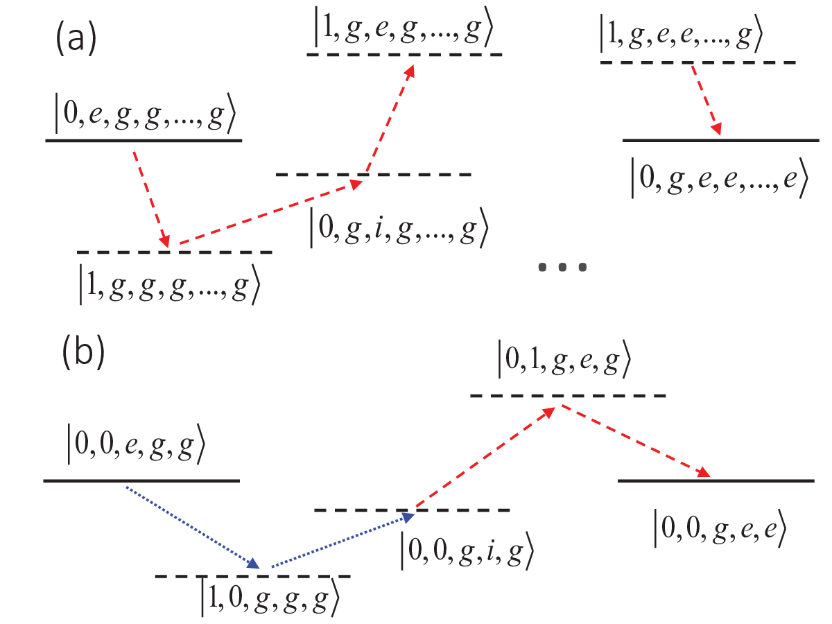
To illustrate the mechanism of the above process, we present an example path describing the contribution in th-order perturbation theory to the effective coupling between the bare states and . As depicted in Fig. 3(a), the transition is connected by intermediate virtual transitions, which do not conserve the energy. Furthermore, except for the st and th atoms, each atom serves as a -type three-level system and gives such a transition path contributing to the effective coupling. After running through the position of the atoms (th atom, ) in every possible permutation, the final state and the initial state are connected via different transition paths.
It is worth to mention that: (i) Since our system is initially prepared in state , and satisfies the frequency matching condition, we obtain the resonant effective Hamiltonian under the RWA by neglecting all the fastvarying terms, and keeping only all terms that are time independent [42]. (ii) In our derivation of the effective interaction Hamiltonian, we have eliminated the third level of the atoms and the degrees of the freedom of the cavity mode, which are never populated but nevertheless cause a renormalization and modification of the effective Hamiltonian. Therefore, we give the effective Hamiltonian in the interaction picture in Eq. (7) with respect to the renormalization form of the bare Hamiltonian. Following the recent work of Guanyu Zhu et al. [37], the renormalization form of the bare Hamiltonian in the second-order perturbation theory can be given as
| (8) |
where the denotes the ac-Stark type dispersive shifts for the cavity mode and the denotes the Lamb type level shift for the th atom. These coefficients and can be determined by using the second-order perturbation theory [37]. Certainly, one can further use higher-order perturbation theory to calculate higher-order correction [37].
II.2 Multi-qutrit coupled through multiple cavities
From the transition path shown in Fig. 3(a), we find that with the exception of the atoms involving in the first and the final intermediate virtual transitions, each atom serves as an type three-level system and contributes such a transition path to the effective coupling. This implies that the one cavity mediated multi-atom coupling scheme introduced in Sec. I(A) can be generalized to multi-cavity case.
As a simple example, we consider a circuit-QED setup shown in Fig. 1(b), where the two cavities are coupled to a common atom and each cavity hosts an atom. As shown in Fig. 3(b), we present the transition path in fourth-order perturbation theory leading to the effective coupling between the bare states and , where labels the states of the two cavity modes and three atoms. The path includes four virtual transitions that do not conserve the energy. The virtual transitions involving the two cavity modes are represented by dotted blue and dashed red arrows, respectively. Compared with the one cavity case, for which there are path connecting the two bare states and , there is only one path which contributes to the effective coupling.
Following the same procedure as in Sec. I(A), we now turn to present the quantitatively derivation for the effective coupling among three atoms mediated by the two cavities. By using RWA, the full system can be described by the Hamiltonian ()
| (9) |
where
| (10) |
describes the Hamiltonian of the two cavities (), and the three atoms , respectively. describes the atom-cavity interaction,
| (11) |
Here, and are the creation and annihilation operators for the cavity (s) with frequency , respectively. is the transition frequency for the th atom from ground to excited state , and denote the atom-cavity coupling strengths for the th atom. For simplicity, we have assumed that the nd atom is coupled to the two cavity modes () with the same coupling strength. For easy reference, we set hereafter.
We consider that the system operates in the dispersive regime, and satisfies the frequency matching condition . Following the derivation in Sec. I(A), we can write the effective Hamiltonian in the interaction picture
| (12) |
where are the ladder operators acting on the lowest two levels and of the th atom, and is the effective coupling strength between the three atoms. The effective coupling strength is given as
| (13) |
In principle, the circuit-QED architecture depicted in Fig. 1(b) can also be generalized to more complex setup, e.g., a two-cavity system where cavities are coupled to a common atom and each cavity hosts multiple atoms, and one-dimensional array of the atom-cavity systems depicted in Fig. 1(b). It allows us to prepare entanglement among atoms located in different cavities, which are important for large-scale quantum information processing [43]. Furthermore, it also allows us to engineer different geometries for coupling multiple atoms mediated by virtual photons, which can be used for engineering various lattice systems for quantum simulation [44].
III application
In this section, we applied our results derived in Sec. II to the concrete case. In particular, we will consider applications in three-atom case, and discuss the quantum dynamics of the system with experimental feasible parameters. We would like to mention again that since the third energy level in principle has null population in the whole process, our numerical analysis focus on the quantum dynamics of the lowest two energy levels. Numerical calculation based on the full Hamiltonian under the RWA were performed using the PYTHON package QuTiP [45, 46]. As mentioned earlier in Sec. II(A), we did not give analytic expressions for the dispersive shift of the energy level. However, in the numerical simulation, the effect of frequency shifts can be canceled out by varying frequencies of the atoms (in the present work, the frequency shifts are compensated for by modified frequency for the st atom). Therefore, the frequency matching condition can be fulfilled.
III.1 photon-mediated three-atom interaction: one cavity case
| Qutrit (=2,3) | Frequency () | Coupling strength () | Relaxation rate () |
|---|---|---|---|
| 7.966 | 150 | 0.01 | |
| 12.0 | 150 | 0.01 | |
| 4.034 | 210 | 0.015 | |
| 4.0 | 150 | 0.01 | |
| 7.5 | 150 | 0.01 | |
| 3.5 | 210 | 0.015 |
We consider the system introduced in Sec.II(A) for the case of three atoms. The system can be described by the Hamiltonian in Eq. (4) with . Furthermore, we assume that , and the system is initially prepared in the state . The effective coupling between the three atoms mediated by virtual photon can be described by
| (14) |
where are the ladder operators acting on the lowest two levels and of the th atom, and the is the effective coupling strength between and .
In following discussion, we choose system parameters as the typical values in circuit QED experiments. The frequency of the cavity mode, , with the cavity photon decay rate . The parameter of the three atoms are listed in Table I. We note that we used two identical qutrits (the nd and rd atom) for the numerical simulation. This choice is just for the sake of simplicity. System consisting of three different qutrits can also work. For instance, different qutrits are used for calculating the energy diagram in Fig. 2. The presence of resonant transition indicates that we can still have the interaction.
According to the fourth-order perturbation theory, we can write down the magnitude of the coupling strength [32]
| (15) |
which results . As shown in Table I, we note that since the nd and rd atoms are treated as two identical cyclic three-level systems, there are paths which have equal contributions to the effective coupling between the bare state and .


We numerically simulated the dynamics of the system under the influence of cavity decay and atom relaxation by using the master equation approach (see Appendix B). The numerical calculations have been performed based on the Hamiltonian in Eq. (4) with . Shown in Fig. 4(a) is the time evolution of the atom mean excitation number . It can be observed from this ordinary oscillation between and that two atoms can jointly exchange excitation with just one single atom in a reversible and coherent way. The period of the oscillation is in good agreement with the value calculated based on the effective coupling strength , i.e., . In Fig. 4(b), we also display the population leakage to the third level of the atoms and the bus cavity. During the time evolution, the population leakage in the third level of the atoms can be negligible, and the mean photon number is far less than 1.
Figure 4(a) shows the time evolution of the two-atom correlation function , which describes the quantum correlation between the emitted photons from the two atoms into noncavity modes [31]. We observe that the two-atom correlation function and the atom mean excitation number almost coincide at early time [27]. This is a signature of almost perfect two-atom correlation: if one atom is excited, the other is also excited [31]. We also find that the two-atom correlation function goes almost to zero every time the mean excitation number of the st atom has maximally value. This behavior indicates that the excitation of the st atom does not convert to a single atom (the nd atom or the rd atom) but the two atom jointly [47]. In the Appendix A, we also consider the four-atom case, and obtain similar results.
This virtual photon-mediated three-atom interaction allows for the realization of three-atom entanglement. Figure 4(a) implies that when the system is initialized in state , which labels the three atoms state, the entangled state can be obtained after a time . Moreover, along with the single atom operations, one can create the three-atom GHZ state .
III.2 photon-mediated three-atom interaction: two-cavity case
Here, we give the numerical analysis of the atom-cavity system depicted in Fig. 1(b). Our aim is to give a numerical confirmation of the theoretical demonstration of the two-cavity mediated three-atom interaction discussed in Sec. II(B). The numerical calculations are performed based on the Hamiltonian in Eq. (9). Furthermore, we note that the st and rd atom acted as two-level systems formed by the lowest two levels of the atoms, while the nd atom worked as an -type three-level system in the transition path leading to the three-atom interaction, as shown in Fig. 3(b). Therefore, for simplicity, we can treat the st and rd atom as two two-level systems in the numerical calculations. We would like to mention again that in the following discussion, are the ladder operators acting on the lowest two levels and of the th atom as we defined in Sec. II(B).
In Fig. 5, we show the time evolution of the atom mean excitation number and the two-atom correlation function under the influence of cavity decay and atom relaxation. We also display the population leakage in the third level of the nd atom () and cavity photon population , as shown in Fig. 5(b). For the numerical simulation, the system parameters are chosen as follows, and are resonance frequency of the two cavity modes , respectively. is the transition frequency for the st atom, and is for the rd atom. The transition frequencies of the nd atom are and . , , and are the atom-cavity coupling strengths. The cavity photon decay rate and the atom relaxation rate are , and , respectively.
Similar to the one cavity case, the two-cavity mediated coherent conversion of the st atom excitation to the other two atoms (the nd and rd atoms) can happen determinatively, and the two-atom correlation function also coincide with the atom mean excitation number at early time, as shown in Fig. 5(a). We can find that the period of the oscillation which is calculated based on the effective coupling strength , i.e., , is good agreement with the result of the numerical simulation of the full dynamics. Figure 5(b) demonstrates that the population leakage in the third level of the nd atom can be negligible, and the photon population in the two cavity modes is far less than 1.


IV Conclusion
In summary, we have studied the resonant exchange interaction among three or more atoms via the exchange of virtual photons in circuit QED system consisting of multi atoms strongly coupled to a cavity mode. If the selection rule of the atom transitions is violated, multiple atoms can jointly exchange excitation with just one single atom in a reversible and coherent way. The analytical and numerical results demonstrate that this excitation number nonconserving process can happen with probability approaching one. In addition, we show that the two-cavity mediated three-atom exchange interaction can also be realized in the strong coupling regime.
This process can be exploited for the realization of an efficient atom-atom entanglement source [27, 46] and can also be used for the implementation of novel schemes for the control and manipulation of atom states, e.g., three-qubit gates [48], quantum repetition coding [27] needed for error-correction codes. Furthermore, it is also possible to use the photon-mediated multi-atom interaction to engineer long-distance entangled state and stabilization of pure many-body states of atoms [49].
In practical, the difficulties one may expect to face with these higher order processes depend on the limitations inherent with the decoherence process of the atom (cyclic qutrit). However, with recent experimental progress in circuit QED, especially, superconducting qubits with a long coherence time have been experimentally demonstrated [50, 51, 52, 53, 54], we estimate that our proposed architecture with three or four atoms is feasible with currently available technology.
Acknowledgements.
This work was partly supported by the NKRDP of China (Grant No. 2016YFA0301802) and NSFC (Grants No. 11504165, No. 11474152, and No. 61521001).Appendix A Cavity-photon mediated four-atom interaction
| Qutrit (=2,3,4) | Frequency () | Coupling strength () | Relaxation rate () |
|---|---|---|---|
| 8.9665 | 180 | 0.01 | |
| 21.0 | 180 | 0.01 | |
| 12.0335 | 210 | 0.015 | |
| 3.0 | 150 | 0.01 | |
| 7.0 | 150 | 0.01 | |
| 4.0 | 200 | 0.015 |
In this appendix, we provide a discussion on the photon-mediated four-atom interaction. We consider the system introduced in Sec. II(A) of the main text for the case of four atoms. The system can be described by the Hamiltonian in Eq. (4) with . For easy reference, we set hereafter. Furthermore, we consider that the system is initialized in state , and satisfies the frequency matching condition . The parameter of the four atom are listed in Table II, the resonance frequency of the cavity mode is , and the cavity photon decay rate is .
Under the frequency matching condition, and by using the sixth-order perturbation theory, the system can be described by the effective Hamiltonian (in the interaction picture)
| (16) |
where () are the ladder operators acting on the lowest two levels and of the th atom, and the is the effective coupling strength between and . The magnitude of the effective coupling strength can be written as
| (17) |
After calculation with the above-mentioned system parameters, the effective coupling strength is obtained as . As shown in Table II, we note that since the three atoms (nd, rd, and th atom) are treated as three identical cyclic qutrits, there are paths which have equal contributions to the effective coupling between the bare state and .
As shown in Fig. 6(a), it can be observed from the oscillation of the atom mean excitation number that three atoms can conspire to jointly exchange excitation with one single atom, and the period is good agreement with calculation given by the perturbation theory. The three-atom correlation function and atom mean excitation number are almost coincident at early time [27]. Figure 6(b) shows that the residual population in the third level of the four atoms can be negligible, and the population in the cavity bus is far less than 1.
As we mentioned in Sec. I of the main text, there exist one other type of effective interactions between the four atoms in the fourth-order perturbation terms, namely, the four-spin ring exchange interaction [26, 27, 55]. Noted that the total excitation number is conserved in this case. Therefore, the four-spin ring exchange interaction can be simply captured by the four-atom Tavis-Cummings Hamiltonian within the RWA.


Appendix B the master equation approach
The influence of cavity decay and atom relaxation on the process can be studied by the master equation approach. By including cavity decay and atom relaxation terms, we can write the master equation:
| (18) |
Above, is the reduced density matrix of the system, is the Hamiltonian of the system, , and denote the photon decay rate of the cavity mode () and the relaxation rate of the two level systems, respectively.
References
- [1] C. Cohen-Tannoudji, J. Dupont-Roc, and G. Grynberg, Atom-Photon Interactions: Basic Processes and Applications (Wiley, New York, 1992).
- [2] T. D. Ladd, F. Jelezko, R. Laflamme, Y. Nakamura, C. Monroe, and J. L. O¡¯Brien, Nature (London) 464, 45 (2010).
- [3] H. J. Kimble, Nature 453, 1023 (2008).
- [4] A. Blais, J. Gambetta, A. Wallraff, D. I. Schuster, S. M. Girvin, M. H. Devoret, and R. J. Schoelkopf, Phys. Rev. A 75, 032329 (2007).
- [5] J. Q. You and Franco Nori, Phys. Rev. B 68, 064509 (2003).
- [6] J. Q. You and F. Nori, Nature (London) 474, 589 (2011).
- [7] M. H. Devoret and R. J. Schoelkopf, Science 339, 1169 (2013).
- [8] A. Srensen and K. Mlmer, Phys. Rev. Lett. 82, 1971 (1999).
- [9] A. Imamoglu, D. D. Awschalom, G. Burkard, D. P. DiVincenzo, D. Loss, M. Sherwin, and A. Small, Phys. Rev. Lett. 83, 4204 (1999).
- [10] S.-B. Zheng and G.-C. Guo, Phys. Rev. Lett. 85, 2392 (2000).
- [11] A. Blais, R.-S. Huang, A. Wallraff, S. M. Girvin, and R. J. Schoelkopf, Phys. Rev. A 69, 062320 (2004).
- [12] L. DiCarlo, J. M. Chow, J. M. Gambetta, L. S. Bishop, B. R. Johnson, D. I. Schuster, J. Majer, A. Blais, L. Frunzio, S. M. Girvin, and R. J. Schoelkopf, Nature (London) 460, 240 (2009).
- [13] J. Majer, J. M. Chow, J. M. Gambetta, J. Koch, B. R. Johnson, J. A. Schreier, L. Frunzio, D. I. Schuster, A. A. Houck, A. Wallraff, A. Blais, M. H. Devoret, S. M. Girvin, and R. J. Schoelkopf, Nature (London) 449, 443 (2007).
- [14] L. DiCarlo, M. D. Reed, L. Sun, B. R. Johnson, J. M. Chow, J. M. Gambetta, L. Frunzio, S. M. Girvin, M. H. Devoret, and R. J. Schoelkopf, Nature (London) 467, 574 (2010).
- [15] M. Neeley, R. C. Bialczak, M. Lenander, E. Lucero, M. Mariantoni, A. D. O’Connell, D. Sank, H. Wang, M. Weides, J. Wenner, Y. Yin, T. Yamamoto, A. N. Cleland, and J. M. Martinis, Nature (London) 467, 570 (2010).
- [16] C. H. Bennett and D. P. DiVincenzo, Nature (London) 404, 247 (2000).
- [17] A. M. Chen, S. Y. Cho, and M. D. Kim, Phys. Rev. A 85, 032326 (2012).
- [18] E. Zahedinejad, J. Ghosh, and B. C. Sanders, Phys. Rev. Lett. 114, 200502 (2015).
- [19] E. Barnes, C. Arenz, A. Pitchford, and S. E. Economou. arXiv:1612.09384 (2016).
- [20] H. Weimer, M. Müller, I. Lesanovsky, P. Zoller, and H. P. Büchler, Nat. Phys. 6, 382 (2010).
- [21] A. Mezzacapo, L. Lamata, S. Filipp, and E. Solano, Phys. Rev. Lett. 113, 050501 (2014).
- [22] D. Becker, T. Tanamoto, A. Hutter, F. L. Pedrocchi, and D. Loss, Phys. Rev. A 87, 042340 (2013).
- [23] T. Tanamoto, V. M. Stojanović, C. Bruder, and D. Becker, Phys. Rev. A 87, 052305 (2013).
- [24] E. T. Jaynes and F. W. Cummings, Proc. IEEE 51, 89 (1963).
- [25] M. Tavis and F. W. Cummings, Phys. Rev. 170, 379 (1968).
- [26] G. Zhu, M. Hafezi, and T. Grover, Phys. Rev. A, 94, 062329 (2016).
- [27] R. Stassi, V. Macrì, A. F. Kockum, O. Di Stefano, A. Miranowicz, S. Savasta, and F. Nori, arXiv:1702.00660 (2017).
- [28] J. Bourassa, J. M. Gambetta, A. A. Abdumalikov, O. Astafiev, Y. Nakamura, and A. Blais, Phys. Rev. A 80, 032109 (2009).
- [29] K. K. W. Ma and C. K. Law, Phys. Rev. A 92, 023842 (2015).
- [30] L. Garziano, R. Stassi, V. Macrì, A. F. Kockum, S. Savasta, and F. Nori, Phys. Rev. A 92, 063830 (2015).
- [31] L. Garziano, V. Macrì, R. Stassi, O. Di Stefano, F. Nori, and S. Savasta, Phys. Rev. Lett. 117(4), 043601 (2016).
- [32] A. F. Kockum, A. Miranowicz, V. Macrì, S. Savasta, and F. Nori, arXiv:1701.05038 (2017).
- [33] A. F. Kockum, V. Macrì, L. Garziano, S. Savasta, and F. Nori, arXiv:1701.07973 (2017).
- [34] T. Niemczyk, F. Deppe, H. Huebl, E. P. Menzel, F. Hocke, M. J. Schwarz, J. J. García-Ripoll, D. Zueco, T. Hümmer, E. Solano, A. Marx, and R. Gross, Nature Phys. 6, 772 (2010).
- [35] P. Forn-Díaz, J. Lisenfeld, D. Marcos, J. J. García-Ripoll, E. Solano, C. J. P. M. Harmans, and J. E. Mooij, Phys. Rev. Lett. 105, 237001 (2010).
- [36] A. Fedorov, A. K. Feofanov, P. Macha, P. Forn-Díaz, C. J. P. M. Harmans, and J. E. Mooij, Phys. Rev. Lett. 105, 060503 (2010).
- [37] G. Zhu, D. G. Ferguson, V. E. Manucharyan, and J. Koch, Phys. Rev. B 87, 024510 (2013).
- [38] Y.-X. Liu, J. Q. You, L. F. Wei, C. P. Sun, and F. Nori, Phys. Rev. Lett. 95, 087001 (2005).
- [39] V. E. Manucharyan, J. Koch, L. I. Glazman, and M. H. Devoret, Science 326, 113 (2009).
- [40] M. R. Delbecq, L. E. Bruhat, J. J. Viennot, S. Datta, A. Cottet, and T. Kontos, Nat. Commun. 4, 1400 (2013).
- [41] T. Yamamoto, K. Inomata, K. Koshino, P.-M. Billangeon, Y. Nakamura, and J. S. Tsai, New J. Phys. 16, 015017 (2014).
- [42] C. K. Law, Phys. Rev. A 49, 433 (1994).
- [43] C. P. Yang, Q. P. Su, S. B. Zheng, and F. Nori, New J. Phys. 18, 013025 (2016).
- [44] D. I. Tsomokos, S. Ashhab, and F. Nori, Phys. Rev. A 82, 052311 (2010).
- [45] J. R. Johansson, P. D. Nation, and F. Nori, Compu. Phys. Commun. 183, 1760 (2012).
- [46] J. R. Johansson, P. D. Nation, and F. Nori, Compu. Phys. Comm. 184, 1234 (2013).
- [47] L. Garziano, R. Stassi, V. Macrì, A. F. Kockum, S. Savasta, and F. Nori, Phys. Rev. A 92, 063830 (2015).
- [48] C. T. Rigetti, Ph.D. thesis, Yale University, New Haven, Connecticut, 2009.
- [49] C. Aron, M. Kulkarni, and H. E. Türeci, Phys. Rev. X 6, 011032 (2016)
- [50] F. Yan, S. Gustavsson, A. Kamal, J. Birenbaum, A. P. Sears, D. Hover, T. J. Gudmundsen, D. Rosenberg, G. Samach, S. Weber, J. L. Yoder, T. P. Orlando, J. Clarke, A. J. Kerman, and W. D. Oliver, Nat.Commun. 7, 12964 (2016).
- [51] J.-L. Orgiazzi, C. Deng, D. Layden, R. Marchildon, F. Kitapli, F. Shen, M. Bal, F. Ong, and A. Lupascu, Phys. Rev. B 93, 104518 (2016).
- [52] M. Stern, G. Catelani, Y. Kubo, C. Grezes, A. Bienfait, D. Vion, D. Esteve, and P. Bertet, Phys. Rev. Lett. 113, 123601 (2014).
- [53] I. M. Pop, K. Geerlings, G. Catelani, R. J. Schoelkopf, L. I. Glazman, and M. H. Devoret, Nature (London) 508, 369 (2014).
- [54] U. Vool, I. M. Pop, K. Sliwa, B. Abdo, C. Wang, T. Brecht, Y. Y. Gao, S. Shankar, M. Hatridge, G. Catelani, M. Mirrahimi, L. Frunzio, R. J. Schoelkopf, L. I. Glazman, and M. H. Devoret, Phys. Rev. Lett. 113, 247001 (2014)
- [55] M. Sameti, A. Potocnik, D. E. Browne, A. Wallraff, and M. J. Hartmann, Phys. Rev. A 95, 042330 (2017).