Joint and Competitive Caching Designs in Large-Scale Multi-Tier Wireless Multicasting Networks
Abstract
Caching and multicasting are two promising methods to support massive content delivery in multi-tier wireless networks. In this paper, we consider a random caching and multicasting scheme with caching distributions in the two tiers as design parameters, to achieve efficient content dissemination in a two-tier large-scale cache-enabled wireless multicasting network. First, we derive tractable expressions for the successful transmission probabilities in the general region as well as the high SNR and high user density region, respectively, utilizing tools from stochastic geometry. Then, for the case of a single operator for the two tiers, we formulate the optimal joint caching design problem to maximize the successful transmission probability in the asymptotic region, which is nonconvex in general. By using the block successive approximate optimization technique, we develop an iterative algorithm, which is shown to converge to a stationary point. Next, for the case of two different operators, one for each tier, we formulate the competitive caching design game where each tier maximizes its successful transmission probability in the asymptotic region. We show that the game has a unique Nash equilibrium (NE) and develop an iterative algorithm, which is shown to converge to the NE under a mild condition. Finally, by numerical simulations, we show that the proposed designs achieve significant gains over existing schemes.
Index Terms:
Cache, multicast, multi-tier wireless network, stochastic geometry, optimization, game theory, Nash equilibriumI Introduction
The rapid proliferation of smart mobile devices has triggered an unprecedented growth of the global mobile data traffic. Multi-tier wireless networks have been proposed as an effective way to meet the dramatic traffic growth by deploying different tiers of point of attachments (POAs), e.g., base stations (BSs) or access points (APs) together, to provide better time or frequency reuse. In general, there are two scenarios, depending on whether different tiers are managed by the same operator. One typical example for the scenario of the same operator is deploying short range small-BSs together with traditional macro-BSs, i.e., heterogeneous wireless networks (HetNets). One typical example for the scenario of different operators is deploying IEEE 802.11 APs of different owners. To further reduce the load of the core network, caching at POAs in multi-tier wireless networks is recognized as a promising approach.
Caching in cache-enabled multi-tier wireless networks for the case of the same operator is considered in many works. Cache-enabled multi-tier wireless networks with fixed topologies are considered in some of them. For example, in [1, 2, 3], the authors consider the optimal content placement at small-BSs to minimize the expected downloading time for files at the macro-BS in a single macro-cell with multiple small-cells. Note that [1, 2, 3] do not capture the stochastic natures of channel fading and geographic locations of POAs and users, and the obtained results in [1, 2, 3] may not be applied to real networks. To address these limitations, large-scale cache-enabled multi-tier wireless networks are considered in some other works, using tools from stochastic geometry. For example, in [4, 5, 6], the authors consider caching the most popular files at each small-BS in large-scale cache-enabled small-cell networks or HetNets. In [7], the authors propose a partition-based combined caching design in a large-scale cluster-centric small-cell network. In [8] and [9], the authors consider random caching of a uniform distribution at small-BSs in a large-scale cache-enabled HetNet and a large-scale cache-enabled small-cell network, respectively. In [10], each macro-BS caches the most popular files and each small-BS randomly caches popular files in a large-scale cache-enabled HetNet. Note that the focuses in [4, 5, 6, 7, 8, 9, 10] are only on performance analysis of some simple caching designs, which may not provide performance guarantee. In [11, 12, 13, 14], the authors consider random caching and focus on the analysis and optimization of the probability that the signal-to-interference plus noise ratio (SINR) of a typical user is above a threshold, in a large-scale cache-enabled multi-tier wireless network. In [11], the authors consider two architectures (i.e., an always-on architecture and a dynamic on-off architecture), and formulate the optimization problem for each architecture, which is convex. For each problem, the closed-form optimal solution is obtained. In [12], the authors consider two cooperative transmission schemes, and formulate the optimization problem under each scheme, which is nonconvex in the general case. For each problem, a stationary point is obtained using the standard gradient projection method. For [13, 14], in a special case where all tiers have the same threshold, the optimization problem is convex and the optimal solution is obtained; in the general case, the problem is nonconvex. In [14], the nonconvex problem is simplified to a convex one and the optimal solution to the simplified convex problem is used as a sub-optimal solution to the original nonconvex problem. In [15], the authors propose a random caching design, and focus on the maximization of the cache hit probability. The optimization problem is convex and the closed-form optimal solution is obtained. Note that [11, 12, 15, 13, 14] focus only on the typical user and do not consider the resource sharing among multiple users.
Some works consider competitive caching among different POAs, using game theory. For instance, in [16], the authors consider an Exact Potential Game among cache-enabled femto-BSs where each femto-BS maximizes the expected number of its served users, prove the existence of Nash equilibrium (NE) and propose a convergent algorithm to obtain a NE. In [17], the authors consider a mean-field game among cache-enabled small-BSs where each small-BS minimizes its long run average cost, and obtain the unique mean field equilibrium. For example, in [18, 19, 20], the authors consider Stackelberg games among content providers and network operators. Specifically, the content providers rent part of the network resources from the network operators for content delivery to get payment from users. Note that in [16, 19, 20], the authors consider cache-enabled wireless networks with fixed topologies. In [17, 18], large-scale cache-enabled wireless networks are considered; in [17], a large-scale cache-enabled single-tier wireless network is considered; in [18], the authors consider a large-scale cache-enabled multi-tier wireless network, but do not provide a convergent algorithm to find the Stackelberg equilibrium.
On the other hand, enabling multicast service at POAs in multi-tier wireless networks is an efficient way to deliver popular contents to multiple requesters simultaneously by effectively utilizing the broadcast nature of the wireless medium. In our previous work [21], we consider analysis and optimization of a hybrid caching design and a corresponding multicasting design in a large-scale cache-enabled HetNet. The hybrid caching design requires the files stored at macro-BSs and pico-BSs to be nonoverlapping and the files stored at all macro-BSs to be identical. Thus, the spatial file diversity provided by the hybrid caching design is limited, which may cause network performance degradation at some system parameters. In our previous work [22], we consider analysis and optimization of a random caching design and a corresponding multicasting design in a large-scale cache-enabled single-tier network. The proposed random caching design in [22] can offer high spatial file diversity, ensuring good network performance over a wide range of system parameters, but can not be directly applied to HetNets.
In summary, further studies are required to facilitate the design of practical cache-enabled multi-tier wireless multicasting networks for massive content dissemination. In this paper, we consider a random caching and multicasting design with caching distributions in the two tiers as the design parameters to provide high spatial file diversity. We derive tractable expressions for the successful transmission probabilities in the general region as well as the high SNR and high user density region (i.e., the asymptotic region), respectively, utilizing tools from stochastic geometry. Our main contributions are summarized below.
- •
For the case of a single operator for the two tiers, we formulate the optimal joint caching design problem to maximize the successful transmission probability in the asymptotic region, which is a nonconvex problem in general. By using the block successive approximate optimization technique[23], we develop an iterative algorithm to obtain a stationary point. Specifically, by carefully choosing an approximation function, we obtain the closed-form optimal solution to the approximate optimization problem in each iteration. In addition, in the special case of the same cache size, we develop a low-complexity algorithm to obtain a globally optimal solution by extending the method in[14].
- •
For the case of two different operators, one for each tier, we formulate the competitive caching design game where each tier maximizes its successful transmission probability in the asymptotic region. We show that the game has a unique NE and develop an iterative algorithm to obtain the NE. In general, it is quite difficult to guarantee that an iterative algorithm can converge to the NE of a game, especially for a large-scale wireless network. By carefully analyze structural properties of the competitive caching design game, we provide a convergence condition for the proposed iterative algorithm, which holds in most practical scenarios.
- •
Finally, by numerical simulations, we show that the proposed designs achieve significant gains over existing schemes in terms of successful transmission probability and complexity. We also show the caching probabilities of the proposed designs, revealing that the proposed designs offer high spatial file diversity.
II System Model
II-A Network Model
We consider a general large-scale two-tier downlink network consisting of two tiers of POAs, e.g., BSs or APs, as shown in Fig. 1. The two tiers can be managed by a single operator (e.g., HetNet with BSs being POAs) or by two different operators (e.g., IEEE 802.11 APs of two owners).11 1 The network model considered in this paper is similar to that in[21]. But here, we consider a random caching design which is more general and includes the hybrid caching design in [21] as a special case. In addition, different from [13, 14], we specify the random caching design by the caching probabilities of file combinations, so as to investigate the file load distribution and the impact of multicasting. The locations of the POAs in tier and tier are spatially distributed as two independent homogeneous Poisson point processes (PPPs) and with densities and , respectively. The locations of the users are also distributed as an independent homogeneous PPP with density . Each POA in the th tier has one transmit antenna with transmission power , where . For notational convenience, we define and . Each user has one receive antenna. All POAs are operating on the same frequency band with a bandwidth (Hz). Consider a discrete-time system with time being slotted and study one slot of the network. Both path loss and small-scale fading are considered: for path loss, a transmitted signal from either tier with distance is attenuated by a factor , where is the path loss exponent [13, 14]; for small-scale fading, Rayleigh fading channels are adopted [24].
Let denote the set of files in the two-tier network. For ease of illustration, assume that all files have the same size. File popularity is assumed to be identical among all users. Each user randomly requests one file, which is file with probability , where . Thus, the file popularity distribution is given by , which is assumed to be known apriori[13, 14].22 2 Note that file popularity evolves at a slower timescale and learning methodologies can be employed to track the evolution of file popularity over time. In addition, without loss of generality (w.l.o.g.), assume . The two-tier network consists of cache-enabled POAs. In the th tier, each POA is equipped with a cache of size to store different popular files out of .
We say every different files form a combination. Thus, there are in total different combinations, each with different files. Let denote the set of combinations. Combination can be characterized by an -dimensional vector , where if file is included in combination of tier and otherwise. Note that there are 1’s in each . Denote as the set of files contained in combination of tier .

II-B Caching
To provide high spatial file diversity, we consider a random caching design in the cache-enabled two-tier network where the caching distributions in the two tiers may be different, as illustrated in Fig. 1. The probability that combination is stored in each POA of tier is , where satisfies
| (1) |
A random caching design in the tier is specified by the caching distribution . Let denote the set of combinations containing file . Let
| (2) |
denote the probability that file is stored at a POA in the th tier. Therefore, the random caching design in the large-scale cache-enabled two-tier network is fully specified by the design parameters . In this paper, we focus on serving cached files at POAs to get first-order insights into the design of cache-enabled wireless networks, as in [25, 22, 21, 14, 13]. POAs may serve uncached files through other service machanisms, the investigation of which is beyond the scope of this paper.
Remark 1
Note that the random caching design considered in this paper is a generalization of the caching design where the most popular files are stored at each POA and the hybrid caching design proposed in [21]. In particular, by choosing the design parameters such that for all and for all , where , the proposed random caching design turns to the design caching the most popular files[7, 9]. In addition, by choosing the design paprameters in a certain manner, the proposed random caching design can reflect identical caching in the st tier, random caching in the nd tier and nonoverlapping caching across the two tiers, and hence incorporate the hybrid caching design in[21] as a special case. Therefore, by carefully designing , the proposed random caching design can achieve better performance than the two designs. Later, we shall see the advantage of the proposed random design in Section VI.
II-C Multicasting
Consider a user requesting file . If file is not stored in any tier, the user will not be served. Otherwise adopt the following user association rule: i) if file is stored only in the th tier, the user is associated with the nearest POA in the th tier storing file ; ii) if file is stored in both tiers, the user is associated with the POA which stores file and provides the maximum long-term average received power (RP) among all the POAs [14, 13].
Remark 2
We consider multicasting in the large-scale cache-enabled two-tier network. Consider a POA serving requests for different files. Then, it transmits each of the files only once to concurrently serve users requesting the same file, at a rate (bit/second) and over of the total bandwidth using frequency division multiple access (FDMA). As a matter of fact, both multicast and unicast may happen (with different probabilities). Without loss of generality, as in [21], we refer to this transmission as multicast. Note that, by avoiding transmitting the same file multiple times to multiple users, this content-centric multicast can improve the efficiency of the utilization of the wireless medium and reduce the load of the wireless network, compared to the traditional connection-based unicast[24]. From the above illustration, we can see that the proposed multicasting design is also affected by the proposed caching design. Therefore, the design parameters affect the performance of the random caching and multicasting design.
II-D Performance Metric
In this paper, we study w.l.o.g. the performance of a typical user , which is located at the origin. Suppose requests file . Let denote the index of the tier with which is associated, and let denote the other tier. Let denote the index of the serving POA of . We denote and as the distance and the small-scale channel between POA and , respectively. We assume the complex additive white Gaussian noise of power (evaluated over the entire frequency band) at . For analytical tractability, as in [22] and [21], we assume all POAs are active for serving their own users. This corresponds to the worst-case interference strength for the typical user.33 3 The performance obtained under this assumption provides a lower bound on the performance of the practical network where some void POAs may be shut down. When requests file and file is transmitted by POA , the SINR of is given by44 4 The bandwidth for serving is random, and affects the signal, interference and noise power experienced at in the same manner, i.e., linearly. Thus, we can use the signal and noise power over the whole frequency band in calculating [21].
| (3) |
Note that, as in[7, 21], the transmitted symbols of file from POA are treated as the desired signal, while the transmitted symbols of file from other POAs are regarded as interference.55 5 The received signals from all the POAs transmitting file may not be perfectly synchronized due to the large difference in distances from these POAs to [26]. When (i.e., may be associated with tier ), let denote the number of different cached files requested by the users associated with POA . Note that is a discrete random variable, whose probability mass function (p.m.f.) depends on , and the design parameters .
The file can be decoded correctly at if the channel capacity between BS and is greater than or equal to . Requesters are mostly concerned about whether their desired files can be successfully received. Therefore, we adopt the probability that a randomly requested file by is successfully transmitted, referred to as the successful transmission probability, as the network performance metric[21]. Let denote the probability that requesting file is associated with tier . By total probability theorem, the successful transmission probability under the considered scheme is
| (4) |
where represents the probability that a randomly requested file by is successfully transmitted from a POA in tier , also referred to as the successful transmission probability of tier .66 6 Note that the expression of the successful transmission probability in (4) is different from the performance metrics in [21] and [24].
III Performance Analysis
In this section, we first analyze the successful transmission probability in the general region. Then, we analyze the successful transmission probability in the asymptotic region.
III-A Performance Analysis in General Region
In this subsection, we analyze the successful transmission probability in the general region (i.e., the general SNR and general user density region), using tools from stochastic geometry. First, the user association probability can be found in[14, 13] and is provided here for completeness:
| (5) |
File load and SINR are correlated in a complex manner in general, as POAs with larger association regions have higher file load and lower SINR (due to larger user to POA distances) [27]. For the tractability of the analysis, as in[22, 21, 27], the dependence is ignored, i.e.,
| (6) |
To obtain the conditional p.m.f. of given by generalizing the methods for calculating the p.m.f. of file load in[21], we need the probability density function (p.d.f.) of the size of the Voronoi cell of BS w.r.t. file when contains combination , where . However, since this p.d.f. is very complex and still unknown, we adopt the widely used approach in the existing literature[27, 24, 22, 21] and approximate this p.d.f. based on a tractable approximation of the p.d.f. of the size of the Voronoi cell to which a randomly chosen user belongs[28]. Under this approximation, the conditional p.m.f. of is given in the following lemma.
Lemma 1 (Conditional p.m.f. of )
The conditional p.m.f. of given is given by
| (7) |
where , and77 7 Note that .
| (8) | ||||
| (9) |
Proof:
Please refer to Appendix A. ∎
| (10) | ||||
| (11) | ||||
| (12) | ||||
| (13) |
Theorem 1 (Performance)
From Theorem 1, we can see that in the general region, the physical layer parameters , , , , , , and the design parameters jointly affect the successful transmission probability . The impacts of the physical layer parameters and the design parameters on are coupled in a complex manner.
III-B Performance Analysis in Asymptotic Region
The gain of multicasting over unicasting increases with user density[21]. In this subsection, to obtain design insights into caching and multicasting, we analyze the asymptotic successful transmission probability in the high SNR and high user density region. Note that in the rest of the paper, when considering the asymptotic region (i.e., the high SNR and user density region), we assume and while fixing the power ratio, i.e., (). In addition, in the high user density region where , the discrete random variable in distribution. From Theorem 1, we can derive the successful transmission probability in the asymptotic region.
Corollary 1 (Asymptotic Performance)
Proof:
Please refer to Appendix B. ∎

Note that and ; when (corresponding to the full file load case), and become functions of and instead of and . In addition, the asymptotic successful transmission probability in Corollary 1 and the performance metric in[13, 14] have different meanings, although they share similar forms. From Corollary 1, we can see that in the high SNR and high user density region, the impact of the physical layer parameters , , and , captured by , and , and the impact of the design parameters on can be easily separated. In most practical cases, . Thus, we consider in the rest of the paper.
Fig. 2 verifies Theorem 1 and Corollary 1, and demonstrates the accuracy of the approximation adopted. Fig. 2 also indicates that provides a simple and good approximation for in the high SNR (e.g., dB) and the high user density region (e.g., ).
In the asymptotic region, from [21], we know that the constraints on in (1) and (2) can be equivalently rewritten as , where is defined as
| (18) |
To obtain design insights into caching in large-scale multi-tier wireless multicasting networks, in Section IV and Section V, we focus on the joint and competitive caching designs in the asymptotic region, respectively.
IV Joint Caching Design
In this section, we consider the case that the two tiers of POAs are managed by a single operator, e.g., as in a HetNet. We first formulate the optimal joint caching design problem to maximize the successful transmission probability in the asymptotic region. Then, we develop an algorithm to obtain a stationary point.
IV-A Optimization Problem Formulation
In this subsection, we formulate the optimal joint caching design problem to maximize the successful transmission probability by optimizing the caching distributions of the two tiers, i.e., .
Problem 1 maximizes a differentiable (nonconcave in general) function over a convex set, and it is thus nonconvex in general. Note that Problem 1 and Problem 0 in [14] are mathematically equivalent, although this paper and [14] have different scopes. In the following subsection, we propose an efficient algorithm to solve Problem 1. In contrast, [14] simplifies the nonconvex problem to a convex one, and uses the optimal solution to the simplified problem as a sub-optimal solution to the original problem, which may not provide performance guarantee.
IV-B Algorithm Design
Recall that Problem 1 is to maximize a differentiable (nonconcave in general) function over a convex set. We can obtain a stationary point of Problem 1 using the gradient projection method with a diminishing stepsize[29, pp. 227], as summarized in Algorithm 1 for completeness. In Algorithm 1, the diminishing stepsize satisfies as , and . In addition, Step 3 is the projection of onto set . It is shown in [29, pp. 229] that the sequence generated by Algorithm 1 converges to a stationary point of Problem 1. Note that a stationary point is a point that satisfies the necessary optimality conditions of a nonconvex optimization problem, and it is the classic goal in the design of iterative algorithms for nonconvex optimization problems. However, the rate of convergence of Algorithm 1 is strongly dependent on the choices of stepsize . If it is chosen improperly, it may take a large number of iterations for Algorithm 1 to meet some convergence criterion.
To address the above problem, in this subsection we propose an iterative algorithm to obtain a stationary point of Problem 1 more efficiently. This algorithm is based on the block successive upper-bound minimization algorithm originally proposed in[23]. It alternatively updates and by maximizing an approximate function of , which is successively refined so that eventually the iterative algorithm can converge to a stationary point of Problem 1. Specifically, at iteration , we update the caching distribution of the th tier by maximizing the approximate function of given the caching distribution of the th tier, and fix the caching distribution of the th tier, where .
For notational convenience, we define
| (19) |
At iteration , choose to be an approximate function of , where is given by
| (20) |
Note that the first concave component function of , i.e., is left unchanged, and only the second nonconcave (actually convex) component function, i.e., is linearized at . This choice of the approximate function is beneficial from several aspects. Firstly, it can guarantee the convergence of the algorithm to a stationary point of Problem 1, which will be seen in Theorem 2. Secondly, the partial concavity of the original objective function is preserved, and the resulting algorithm typically converges much faster than Algorithm 1, where all component functions are linearized and no partial concavity is exploited. Thirdly, it yields a closed-form optimal solution to the optimization problem at each iteration, which will be explained in Lemma 2. Specifically, is strictly concave on for any given , and satisfies88 8 Note that (21) holds since and have the same value at the point where is defined, i.e., . (22) holds since is a convex function of for any given .
| (21) | ||||
| (22) |
The conditions in (21) and (22) imply that is a tight lower-bound of . The differentiability of guarantees that the first-order behavior of is the same as locally. At each iteration , we update the caching distribution of the th tier given the caching distribution of the th tier by solving the following problem, and fix the caching distribution of the th tier, where .
Problem 2 (Optimization at Iteration )
Problem 2 is a convex optimization problem and Slater’s condition is satisfied, implying that strong duality holds. Using KKT conditions, we can obtain the closed-form optimal solution to Problem 2, as shown in the following lemma.
Lemma 2 (Optimal Solution to Problem 2)
For all , the optimal solution to Problem 2 is given by
where and is the Lagrange multiplier that satisfies
Note that can be efficiently obtained by using bisection search.
The details of the proposed iterative algorithm are summarized in Algorithm 2. Based on the conditions in (21) and (22), we show the convergence and optimality of Algorithm 2.
Theorem 2 (Convergence and Optimality of Algorithm 2)
Proof:
Please refer to Appendix C. ∎
Different from Algorithm 1, Algorithm 2 does not rely on a stepsize. Thus, Algorithm 2 may have more robust convergence performance than Algorithm 1, as we shall illustrate later in Fig. 3.
In the rest of this subsection, we consider a special case where . In this case, , and . In addition, can be further simplified as
| (23) |
which is a concave function of . Thus, Problem 1 becomes a convex optimization problem, and a (globally) optimal solution can be obtained by standard convex optimization methods such as interior-point methods. However, when is very large, standard convex optimization methods may not scale very well. Motivated by[14], by exploring structural properties of Problem 1 in this case, we develop a low-complexity algorithm to obtain an optimal solution. The method consists of two stages. In the first stage, we solve a relaxed version of Problem 1 to obtain a system of linear equations of an optimal solution to Problem 1. This stage is the same as that in[14], and is included for completeness. Denote , where . Specifically, Problem 1 can be relaxed as follows.
The optimal soluton to Problem 3 is given by [14, Proposition 3], i.e.,
| (24) |
where is the Lagrange multiplier that satisfies
| (25) |
Note that can be efficiently obtained by using bisection search. In addition, by Proposition 4 in [14], we know that the optimal solution to Problem 3 and an optimal solution to Problem 1 satisfy a system of linear equations:
| (26) |
In the second stage, we solve the system of linear equations given in (26) to obtain an optimal solution to Problem 1. In our case, we can easily show that
| (27) |
is a solution to the system of linear equations in (26). This stage is different from that in[14], as we can directly obtain using the closed-form expression in (27), due to . The details are summarized in Algorithm 3. Note that the complexity of Algorithm 3 is close to that of one iteration of Algorithm 2. Thus, the complexity of Algorithm 3 is much lower than Algorithm 2.
V Competitive Caching Design
In this section, we study the scenario that the two tiers of POAs are managed by two different operators, e.g., IEEE 802.11 APs of two owners. The two different operators have their own interests and thus cannot be jointly managed. Besides, one operator may be sacrificed in order to achieve the maximum total utility. Therefore, we propose a game theoretic approach and adopt a NE as a desirable outcome. We first formulate the competitive caching design for the two different operators within the framework of game theory. Then, we characterize a NE of the game and develop an algorithm to obtain a NE.
V-A Game Formulation
In this subsection, we formulate the competitive caching design for the two different operators within the framework of game theory. We consider a strategic noncooperative game, where the two operators are the players. The utility function of player is the successful transmission probability for tier , i.e., . Each tier competes against the other tier by choosing its caching distribution (i.e., strategy or action) in the set of admissible strategies to maximize its utility function, i.e., .
Problem 4 (Competitive Caching Game)
For all , we have
| s.t. |
A solution, i.e., a NE,99 9 A NE is reached when each player, given the strategy profiles of the others, does not get any performance increase by unilaterally changing his own strategy[30]. of game is defined as follows.
Definition 1 (Nash Equilibrium of Game )
A (pure) strategy profile is a NE of game if
| (28) |
By Definition 1, we know that a NE of game is given by the following problem.
Problem 5 (NE of Game )
For all , we have
| s.t. |
V-B Nash Equilibrium
In this subsection, we characterize a NE of game . First, we show the existence and uniqueness of the NE of game .
Lemma 3 (Existence and Uniqueness of the NE of Game )
There exists a unique NE of game .
Proof:
Please refer to Appendix D. ∎
We now obtain the closed-form expression of the unique NE of game . Since is strictly concave on for any given , Problem 5 is convex and Slater’s condition is satisfied, implying that strong duality holds. Using KKT conditions, we can solve Problem 5 and show Lemma 4.
Lemma 4 (NE of Game )
Game has a unique NE which is given by
where for all , is the Lagrange multiplier that satisties
Remark 3
The file popularity distribution and the physical layer parameters (captured in , and ) jointly affect . Given and , , the physical layer parameters (captured in , and ) affect the caching probabilities of all the files in the same way, while the popularity of file (i.e., ) only affects the caching probability of file (i.e., ) [22].
V-C Algorithm Design
In this subsection, we develop an iterative algorithm to obtain the NE of game . It alternatively updates while is fixed and while is fixed, by solving the following problem at each iteration .
Problem 6 (Optimization at Iteration )
For player , we have
| s.t. |
Similar to Problem 5, using KKT conditions, we can obtain the closed-form expression of the unique optimal solution to Problem 6. We present it below for completeness.
Lemma 5 (The Optimal Solution to Problem 6)
For all , the optimal solution to Problem 6 is given by
where is the Lagrange multiplier that satisfies
Note that Problem 5 and Problem 6 in Lemma 5 share similar forms. Thus, the NE of game in Lemma 4 and the solution to Problem 6 share similar forms. Based on the optimal solution to Problem 6, at iteration , we update the strategy of player , and fix the strategy of player , where . The details for obtaining the NE of game is summarized in Algorithm 4.
Note that in general, it is quite difficult to guarantee that an iterative algorithm can converge to the NE of a game, especially for a large-scale wireless network. By carefully analyze structural properties of the competitive caching design game, we provide a convergence condition for Algorithm 4.
Theorem 3 (Convergence of Algorithm 4)
VI Numerical Results
In this section, we first illustrate the convergence and complexity of the proposed algorithms. Then, we compare the successful transmission probabilities and caching probabilities of the proposed algorithms with those of existing solutions. In the simulation, we choose , , , , , and . We assume that the popularity follows Zipf distribution, i.e., , where is the Zipf exponent.




VI-A Convergence and Complexity
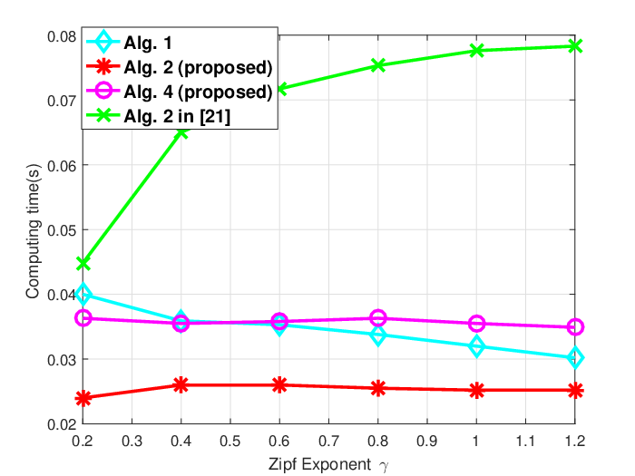
In this subsection, we show the convergence and complexity of the proposed algorithms. Fig. 3 illustrates the successful transmission probability versus the number of iterations when and . From Fig. 3, we can observe that the rate of convergence of Algorithm 1 is strongly dependent on the choices of stepsize . In addition, Algorithm 2 and Algorithm 4 have more robust convergence performance than Algorithm 1, as they do not rely on a stepsize. Fig. 4 illustrates the computing time versus the cache size and the Zipf exponent when and . From Fig. 4, we can observe that the computing times of all the algorithms do not change much with or , and the computing times of the proposed algorithms are shorter than that of Algorithm 2 in [21] which is to obtain an asymptotically optimal hybrid caching design. These observations demonstrate the advantage of the proposed algorithms in terms of complexity.


VI-B Successful Transmission Probabilities and Caching Probabilities
In this subsection, we compare the successful transmission probabilities and caching probabilities of the proposed joint and competitive caching designs with those of three baselines. Baseline 1 (most popular) refers to the design in which each POA in tier stores the most popular files [4, 5, 6]. Baseline 2 (i.i.d. file popularity) refers to the design in which each POA in tier randomly stores files, in an i.i.d. manner with file being selected with probability [31]. Baseline 3 (hybrid caching) refers to the hybrid caching design obtained by Algrithm 2 in [21]. The three baseline schemes also adopt the same multicasting scheme as in our design. Fig. 5 illustrates the successful transmission probability versus the cache size and the Zipf exponent , respectively. From Fig. 5, we can observe that as and increase, the successful transmission probability of each scheme increases. We can also observe that the two proposed designs outperform all the three baseline schemes. In addition, we can see that when or is large, the two proposed designs reduce to the most popular caching design. When or is small, the two proposed designs perform similarly as the hybrid caching design. These observations show that the two proposed designs can well adapt to the changes of the system parameters and can wisely utilize storage resources.
Fig. 6 illustrates the caching probabilities for the proposed joint caching design, competitive caching design and the hybrid caching design. From Fig. 6, we observe that under the proposed joint caching design and the hybrid caching design, when is above (below) some threshold, POAs of tier (POAs of tier ) cache the most popular files as they can offer relatively higher received powers. Recall that under the hybrid caching design, the files stored in the two tiers are non-overlapping, while the proposed joint caching design and competitive caching design allow a file to be stored in the two tiers. By comparing the caching probabilities under the three designs, we can see that the joint caching design and the competitive caching design offer much higher spatial file diversity, leading to higher successful transmission probabilities.
VII Conclusion
In this paper, we considered a random caching and multicasting scheme in a two-tier large-scale cache-enabled wireless multicasting network, operated by a single operator or two different operators. First, we derived tractable expressions for the successful transmission probabilities in the general region and the asymptotic region, respectively. Then, we formulated the optimal joint caching design problem in the asymptotic region. We develop an iterative algorithm, which is shown to converge to a stationary point. Next, we formulated the competitive caching design game in the asymptotic region, obtained the unique NE of the game and developed an iterative algorithm, which is shown to converge to the NE under a mild condition. Finally, by numerical simulations, we showed that the two proposed designs achieve significant gains over existing schemes, in terms of successful transmission probability and complexity.
Appendix A: Proof of Lemma 1
Appendix B: Proof of Corollary 1
Appendix C: Proof of Theorem 2
We show that the conditions in Theorem 2 (a) of [23] hold. i) By noting that (21) and (22) hold and is continuous and differentiable, we know that Assumption 2 in [23] is satisfied and is regular at any point in [23]. ii) Since is strictly concave on for any given , Problem 2 has a unique solution for any given . Therefore, by Theorem 2 (a) in[23], we can prove Theorem 2.
Appendix D: Proof of Lemma 3
First, we use Proposition 20.3 in [33] to prove the existence of NE of game . It is obvious that for all , the set of admissible strategies is nonempty, compact and convex, and the utility function is a continuous function of . Since is strictly concave on for any given , then is quasi-concave on for any given . Thus, by Proposition 20.3 in [33], we know that there exists at least one NE of game . Next, we prove the uniqueness of NE by Theorem 2 in [34]. By the first-order strict concavity condition, we know that a strictly concave function must be diagonally strictly concave[34]. Thus, by Theorem 2 in [34], we know that there exists a unique NE of game .
Appendix E: Proof of Theorem 3
We prove the convergence of Algorithm 4 by verifying the conditions in Theorem 1 of[35]. i) It can be easily seen that for all , is strictly concave on for any given and is second-order Fréchet differentiable[36]. ii) By Lemma 5, we know that there exists an optimal solution to Problem 6 for any given . iii) To guarantee the convergence of Algorithm 4, it remains to show that
| (32) |
holds for any and . Here, denotes the spectral norm [36]. By Corollary 1, we have
| (33) |
where is obtained by the definition of second-order derivative, is obtained by the definition of spectral norm, is obtained based on the formula , and is obtained due to
| (34) | ||||
| (35) |
References
- [1] K. Shanmugam, N. Golrezaei, A. Dimakis, A. Molisch, and G. Caire, “Femtocaching: Wireless content delivery through distributed caching helpers,” Information Theory, IEEE Transactions on, vol. 59, no. 12, pp. 8402–8413, Dec 2013.
- [2] J. Li, Y. Chen, Z. Lin, W. Chen, B. Vucetic, and L. Hanzo, “Distributed caching for data dissemination in the downlink of heterogeneous networks,” IEEE Transactions on Communications, vol. 63, no. 10, pp. 3553–3568, Oct 2015.
- [3] Y. Cui, F. Lai, S. Hanly, and P. Whiting, “Optimal caching and user association in cache-enabled heterogeneous wireless networks,” in Global Communications Conference (GLOBECOM), 2016 IEEE. IEEE, 2016, pp. 1–6.
- [4] E. Bastu, M. Bennis, M. Kountouris, and M. Debbah, “Cache-enabled small cell networks: Modeling and tradeoffs,” EURASIP Journal on Wireless Communications and Networking, 2015.
- [5] D. Liu and C. Yang, “Cache-enabled heterogeneous cellular networks: Comparison and tradeoffs,” in Communications (ICC), 2016 IEEE International Conference on. IEEE, 2016, pp. 1–6.
- [6] C. Yang, Y. Yao, Z. Chen, and B. Xia, “Analysis on cache-enabled wireless heterogeneous networks,” Wireless Communications, IEEE Transactions on, vol. 15, no. 1, pp. 131–145, Jan 2016.
- [7] Z. Chen, J. Lee, T. Q. Quek, and M. Kountouris, “Cooperative caching and transmission design in cluster-centric small cell networks,” IEEE Transactions on Wireless Communications, vol. 16, no. 5, pp. 3401–3415, 2017.
- [8] S. T. ul Hassan, M. Bennis, P. H. J. Nardelli, and M. Latva-aho, “Caching in wireless small cell networks: A storage-bandwidth tradeoff,” IEEE Communications Letters, vol. PP, no. 99, pp. 1–1, 2016.
- [9] S. Tamoor-ul Hassan, M. Bennis, P. H. Nardelli, and M. Latva-Aho, “Modeling and analysis of content caching in wireless small cell networks,” in Wireless Communication Systems (ISWCS), 2015 International Symposium on. IEEE, 2015, pp. 765–769.
- [10] J. Zhang, X. Zhang, M. A. Imran, B. Evans, and W. Wang, “Energy efficiency analysis of heterogeneous cache-enabled 5g hyper cellular networks,” in Global Communications Conference (GLOBECOM), 2016 IEEE. IEEE, 2016, pp. 1–6.
- [11] Y. Chen, M. Ding, J. Li, Z. Lin, G. Mao, and L. Hanzo, “Probabilistic small-cell caching: Performance analysis and optimization,” IEEE Transactions on Vehicular Technology, 2016.
- [12] W. Wen, Y. Cui, F.-C. Zheng, S. Jin, and Y. Jiang, “Random caching based cooperative transmission in heterogeneous wireless networks,” arXiv preprint arXiv:1701.05761, 2017.
- [13] K. Li, C. Yang, Z. Chen, and M. Tao, “Optimization and analysis of probabilistic caching in -tier heterogeneous networks,” arXiv preprint arXiv:1612.04030, 2016.
- [14] J. Wen, K. Huang, S. Yang, and V. O. Li, “Cache-enabled heterogeneous cellular networks: Optimal tier-level content placement,” arXiv preprint arXiv:1612.05506, 2016.
- [15] B. Serbetci and J. Goseling, “On optimal geographical caching in heterogeneous cellular networks,” in Wireless Communications and Networking Conference (WCNC), 2017 IEEE. IEEE, 2017, pp. 1–6.
- [16] Y. Tan, Y. Yuan, T. Yang, Y. Xu, and B. Hu, “Femtocaching in wireless video networks: Distributed framework based on exact potential game,” in Proc. IEEE ICCC. IEEE, 2016, pp. 1–6.
- [17] H. Kim, J. Park, M. Bennis, S.-L. Kim, and M. Debbah, “Ultra-dense edge caching under spatio-temporal demand and network dynamics,” arXiv preprint arXiv:1703.01038, 2017.
- [18] J. Li, J. Sun, Y. Qian, F. Shu, M. Xiao, and W. Xiang, “A commercial video-caching system for small-cell cellular networks using game theory,” IEEE Access, vol. 4, pp. 7519–7531, 2016.
- [19] K. Poularakis, G. Iosifidis, and L. Tassiulas, “A framework for mobile data offloading to leased cache-endowed small cell networks,” in Mobile Ad Hoc and Sensor Systems (MASS), 2014 IEEE 11th International Conference on. IEEE, 2014, pp. 327–335.
- [20] F. Shen, K. Hamidouche, E. Baştuğ, and M. Debbah, “A stackelberg game for incentive proactive caching mechanisms in wireless networks,” arXiv preprint arXiv:1609.02596, 2016.
- [21] Y. Cui and D. Jiang, “Analysis and optimization of caching and multicasting in large-scale cache-enabled heterogeneous wireless networks,” IEEE Trans. Wireless Commun., vol. 16, no. 1, pp. 250–264, 2017.
- [22] Y. Cui, D. Jiang, and Y. Wu, “Analysis and optimization of caching and multicasting in large-scale cache-enabled wireless networks,” IEEE Trans. Wireless Commun., vol. 15, no. 7, pp. 5101–5112, 2016.
- [23] M. Razaviyayn, M. Hong, and Z.-Q. Luo, “A unified convergence analysis of block successive minimization methods for nonsmooth optimization,” SIAM J. Optimization, vol. 23, no. 2, pp. 1126–1153, 2013.
- [24] S. Singh, H. S. Dhillon, and J. G. Andrews, “Offloading in heterogeneous networks: modeling, analysis, and design insights,” IEEE Trans. Wireless Commun., vol. 12, no. 5, pp. 2484–2497, March 2013.
- [25] J. Andrews, F. Baccelli, and R. Ganti, “A tractable approach to coverage and rate in cellular networks,” Communications, IEEE Transactions on, vol. 59, no. 11, pp. 3122–3134, November 2011.
- [26] S. H. Chae, J. Y. Ryu, T. Q. Quek, and W. Choi, “Cooperative transmission via caching helpers,” in Global Communications Conference (GLOBECOM), 2015 IEEE. IEEE, 2015, pp. 1–6.
- [27] S. Singh and J. Andrews, “Joint resource partitioning and offloading in heterogeneous cellular networks,” Wireless Communications, IEEE Transactions on, vol. 13, no. 2, pp. 888–901, Feb 2014.
- [28] S. M. Yu and S.-L. Kim, “Downlink capacity and base station density in cellular networks,” in Modeling Optimization in Mobile, Ad Hoc Wireless Networks (WiOpt), 2013 11th International Symposium on, May 2013, pp. 119–124.
- [29] D. P. Bertsekas, Nonlinear programming. Athena scientific Belmont, 1999.
- [30] G. Scutari, D. Palomar, and S. Barbarossa, “Competitive design of multiuser mimo systems based on game theory: A unified view,” IEEE Journal on Selected Areas in Communications, vol. 26, no. 7, 2008.
- [31] B. B. Nagaraja and K. G. Nagananda, “Caching with unknown popularity profiles in small cell networks,” in Global Communications Conference (GLOBECOM), 2015 IEEE. IEEE, 2015, pp. 1–6.
- [32] S. Singh, H. S. Dhillon, and J. G. Andrews, “Offloading in heterogeneous networks: Modeling, analysis, and design insights,” IEEE Transactions on Wireless Communications, vol. 12, no. 5, pp. 2484–2497, 2013.
- [33] M. J. Osborne and A. Rubinstein, A course in game theory. MIT press, 1994.
- [34] J. B. Rosen, “Existence and uniqueness of equilibrium points for concave n-person games,” Econometrica: Journal of the Econometric Society, pp. 520–534, 1965.
- [35] S. Li and T. Başar, “Distributed algorithms for the computation of noncooperative equilibria,” Automatica, vol. 23, no. 4, pp. 523–533, 1987.
- [36] D. G. Luenberger, Optimization by vector space methods. John Wiley & Sons, 1969.