FIT HE - 17-01
Holographic Cosmology and
Phase Transitions of SYM theory
†Kazuo Ghoroku11
1
gouroku@fit.ac.jp,
∗René Meyer33
3
Rene.Meyer@physik.uni-wuerzburg.de,
and ¶Fumihiko Toyoda44
4
ftoyoda@fuk.kindai.ac.jp
†Fukuoka Institute of Technology, Wajiro, Higashi-ku
Fukuoka 811-0295, Japan
∗Institute for Theoretical Physics and Astrophysics, University of Würzburg, 97074 Würzburg, Germany
¶Faculty of Humanity-Oriented Science and Engineering, Kinki University,
Iizuka 820-8555, Japan
Abstract
We study the time development of strongly coupled supersymmetric Yang Mills (SYM) theory on cosmological Friedmann-Robertson-Walker (FRW) backgrounds via the AdS/CFT correspondence. We implement the cosmological background as a boundary metric fulfilling the Friedmann equation with a four-dimensional cosmological constant and a dark radiation term. We analyze the dual bulk solution of the type IIB supergravity and find that the time-dependence of the FRW background strongly influences the dynamical properties of the SYM theory. We in particular find a phase transition between a confined and a deconfined phase. We also argue that some cosmological solutions could be related to the inflationary scenario.
1 Introduction
The holographic approach [1, 2, 3] to supersymmetric Yang Mills (SYM) theory can be extended from the theory on flat Minkowski space-time to the one on curved boundary background space-times [4, 5, 6, 7]. Such an extension is useful to understand for example the dynamical properties of the SYM theory on cosmologically developing four dimensional (4D) Friedmann-Robertson-Walker (FRW) type space-times. Indeed, the influence of the cosmological evolution on several dynamical properties of the SYM theory such as e.g. the quark-antiquark potential have been clarified in [4, 5, 6, 7]. Since the deconfined phase of QCD behaves in many ways similar to SYM theory at finite temperature, these studies yield interesting information about the behaviour of the quark-gluon plasma in the early universe before big bang nucleosynthesis.
In the holographic approach, the scale factor is undetermined by the bulk equations of motions due to gravity decoupling from the boundary and the boundary metric being nondynamical. For the same reason, the boundary cosmological constant can a priori be any function of time, . In [5, 6], the vacuum state of the SYM theory has been examined by setting to a constant parameter. This is equivalent to set to be a solution of the 4D Friedmann equation with a 4D cosmological constant . It has been found in particular [5, 6] that the ground state of the SYM theory is in the deconfinement and confinement phase for the positive and the negative values of , respectively.
In [7], this analysis has been extended by including a new parameter , the dark radiation constant, into the bulk solution. This parameter has been first introduced in [8, 9] in the context of brane world models, and its origin has been discussed in [10, 11]. From the holographic viewpoint, as shown in [7], the bulk solution is related by a large bulk diffeomorphism to the AdS5-Schwarzschild metric with Hawking temperature set by . The bulk diffeomorphism in particular acts on the boundary metric as a conformal transformation relating the FRW boundary metric to flat Minkowski space-time. Its field theory dual therefore represents a finite temperature SYM state in a FRW universe. In general, the dynamical properties of the dual theory are now controlled by the two parameters, and . In [12], the analysis was extended to time-dependent by assuming the existence of the matter other than the 4D cosmological constant in the boundary space-time, however the time-dependent properties of the SYM state has not been discussed there. It was found [12] that the system is in the deconfinement phase when is large enough even if the boundary cosmological constant is negative. Hence the two parameters and can provide opposite dynamical effects in the theory, as shown in [12, 13].
In this work we extend the analysis to the case where we can see how the state of the SYM system varies with the cosmological development of our universe. Our purpose is to propose a self-consistent procedure how to do it and to find the time dependence of the state of the SYM theory. The procedure is as follows: First, we obtain the energy momentum tensor of the SYM theory, , in the FRW boundary metric from holographic renormalization [14, 15, 16]. Then by using this tensor, the 4D Einstein equations (i.e. the Friedmann equation for the at that point arbitrary scale factor ) with and SYM as a matter are solved to obtain the boundary scale factor . After that, the time development of the SYM state is then analyzed by substituting this back into the bulk solution. We notice that the 4D Einstein equations used here were obtained in [17] from a different holographic regularization procedure by adding a 4D boundary gravitational action. This formulation may be related also to the designer gravity approach of [t, Kiri]o couple two AdS spacetimes together such that at the boundary a gravitational theory is induced.
The solutions of obtained in this way provide a ”sudden” singularity [19] in the 4D boundary space-time at the minimum value of the scale factor . The boundary cosmological constant is found as a two valued function of for . The two branches merge at the minimal value. We then study the solutions for the two cases and separately.
The region of negative 11 1 We should not confusing with . It seems they should be the same. We could see their exact difference and relation in the sction three. is realized in the case of , where we observe the expected phase transition between Wilson loop confinement and deconfinement. The equation of state , where and denote the pressure and energy densities of the SYM fields, is found to be a useful parameter for this the transition. The parameter , which varies with time, characterizes the state of the SYM theory. We found that the critical point of the confinement-deconfinement transition is at exactly . We speculate on why this point is critical in terms of the Virial theorem. For , on the other hand, inflation behavior will be found through this analysis and issues related to their cosmology are discussed.
As for the second branch of the solutions, which cover a larger positive region of , a simple behavior of the solution is obtained, and the relation to the cosmology is discussed. In both cases, the value of is bounded from below when the dark radiation is present. This implies that we need to take into account quantum gravitational effects to approach the dynamics in the region of since the curvature diverges at . In this region, an approach from quantum cosmology in the mini-superspace would be available to resolve the dynamical properties of the system.
The outline of this paper is as follows: In the next section, a bulk space-time is given as a solution of 10D type IIB supergravity, and previous results for the dual of SYM theory in the FRW space-time are reviewed. In the Sec. 3, the procedure to obtain the cosmological time-development of the SYM theory by self-consistently calculating is laid out in detail, and the solutions which cross the (de)confinement transition point are studied. Other kinds of solutions and their relation to the inflationary scenario are discussed in Sec. 4. The solutions, which cover large region, are given in the Sec. 5, and the relation to the cosmology is discussed. Summary and discussions are given in the final, sixth, section.
2 Holography of SYM theory in a FRW metric
We start with ten-dimensional type IIB supergravity retaining the dilaton , axion , as well as the selfdual five form field strength ,
| (2.1) |
All other fields are set to zero, and is Wick rotated to the Euclidean domain [20]. We are going to use the Freund-Rubin ansatz for , [21, 22] to reduce to the five noncompact dimensions.
The equations of motion of the above theory are then solved by an Ansatz for the 10D metric as ,
The five sphere radius is defined via .
The holographic dual to the large gauge theory embedded in 4D space-time with dark energy and ”dark radiation” is solved by the gravity on the following form of the metric,
| (2.2) |
where
| (2.3) |
and or . The arbitrary scale parameter of three space is set hereafter as . The solution is obtained from 10D supergravity of type IIB theory [7, EGR2, 12, 25].
| (2.4) | |||||
| (2.5) |
where
| (2.6) |
and
| (2.7) |
- •
- •
On the other hand, from the holographic viewpoint, it has been cleared that corresponds to the radiation energy of the SYM fields [7]. In the following, we adopt this interpretation.
- •
In general, we can see how the physical quantities of the SYM theory varies with time when the t-dependence of has been given. Our purpose is to find it. Before doing it, we briefly review the results of the previous analysis where the time dependence of is neglected by assuming that it varies very slowly.
2.1 Phase Diagram for const.
The dynamical properties of the theory can be studied under the assumption that varies very slowly compared to the time scale of the dynamics of the SYM theory. [7] 22 2 We should notice the following fact that the solution, constant, is actually found for negative constant and . This is considered as an extremal case of the slowly varying . Since there is no equation to determine in solving the 5D Einstein equations, then there is no constraint on the time dependence of . Then the parameters appearing in the bulk configuration ( and ) can be taken as arbitrary values.
In the case of constant , the factors and of the above solution are written as follows,
| (2.8) | |||||
| (2.9) |
| (2.10) |
In this case, the dynamical properties of the dual 4D SYM theory on the boundary are controlled by the and , or and .
- •
- •
finite and :
For this case, the 5D metric is reduced to the AdS5-Schwarzschild form, in which represents the black hole mass. Then, from the holographic viewpoint, corresponds to the thermal radiation of the SYM fields at a finite temperature [7]. So the system is in the deconfinement phase. - •
From the above two facts, we could suppose that the two parameters, and , compete with each other to realize the opposite phase of the theory, namely the deconfinement and confinement respectively. In fact, we could find the phase transition at a point where these two opposite effects are balanced [7, EGR2, 12, 25, GNI14]. The critical line is given by , where the density of dark radiation and the magnitude of are replaced by and as given by the formula (2.10). The phase diagram of the SYM theory in the FRW space-time is given as in the Fig. 1.
- •
In the deconfinement phase or in the region , the temperature is given as the Hawking temperature of the 5D metric. Then decreases with increasing up to the transition temperature () to the confinement phase. It is given as , which corresponds to the critical line in the Fig. 1.
- •
For positive case, the theory is in the deconfinied chiral symmetric phase. The description of the phase in plane is abbreviated.

2.2 For the case of time dependent
The case of the time independent and is a simple approximation. As shown below, here we solve the 4D Einstein equation to obtain a time dependence of and by using the 4D energy momentum tensor of the SYM theory which is obtained by the holographic method. Then the phase transition line given by (a) in the Fig. 1 is modified to (b), which obeys the following formula,
| (2.11) |
The derivation and the details of this result are given below.
3 Cosmological time development of SYM system
3.1 Holographic Cosmology
As mentioned above, the scale factor can not be determined by the bulk equations of motion. On the other hand, it is obtained as a solution of 4D cosmological equation, where the gravity couples to various matter. Here we give it by solving the 4D Einstein equation which couples to the SYM theory. In the equations, we use the energy momentum tensor of SYM, , which is holographically obtained. Using the obtained in this way, we can see the time-development of the state of the SYM theory.
Here we consider a simple 4D model, in which the matter part is dominated by the SYM fields. The action to be solved is given as
| (3.1) |
where and denote the 4D gravitational constant and cosmological constant respectively. Furthermore, the matter part is written as an effective action which is obtained by integrating out over all quantum fluctuations of the SYM fields under the FRW metric,
| (3.2) |
The factor is obtained by solving the following Einstein equation,
| (3.3) |
where
| (3.4) |
which represents the energy momentum tensor of SYM fields. It includes all quantum corrections of the interacting SYM fields in the background (3.2).
As we mentioned in the introduction, we should notice here that the Eq. (3.3) has been obtained from the holographic regularization procedure with a different boundary condition from the Dirichlet condition by adding an appropriate boundary 4D gravitational action. [17]
The strategy of our holographic approach is given as follows.
(i) First, is given by the holographic method.
3.2 Equations to be solved
The independent equations of (3.3) are obtained as follows
| (3.5) |
| (3.6) |
The first Eq. (3.5) represents the component of (3.3), it is called as Friedmann equation.
Using the above two equations, we obtain the following continuity equation,
| (3.7) |
where is supposed to be written by and as
| (3.8) |
The contents of the above are given as follows [12, 15, 16, 14]
| (3.9) |
| (3.10) |
It is easy to see that the equation (3.7) is satisfied by the above and .
We notice that to solve the Eqs. (3.5) and (3.6) is equivalent to solve Eqs. (3.5) and Eqs. (3.7). On the other hand, the Eq. (3.7) is satisfied for the above as mentioned above. So, our task to do here is to solve the Friedman equation (3.5) to obtain , and the equation to be solved is written as
| (3.11) |
where
| (3.12) |
The equation (3.11) is then solved at first with respect to as follows 33 3 We notice here,
| (3.13) |
In the following, we solve the above equations for and separately. The solutions of the two equations can be connected at a singular point , which is given below.
4 Solution of
4.1 For
The main purpose here is to study the state of the theory in the region of , which is realized for , since a phase transition is expected there. The case of is studied afterward.
The case of is realized for the solution, with negative . In this case, the equation to be solved is written as, In this case, the equation to be solved is written as,
| (4.1) |
We notice . And, here we suppose to cover the region of negative . For the solution of this equation, the value of varies in the range
| (4.2) |
The negative is found for
| (4.3) |
On the other hand, for the case,
| (4.4) |
we found positive . The right hand side of the inequality (4.4) denotes the condition for the reality of , and it provides the minimum of the allowed . It is given as
| (4.5) |
This point is called as ”sudden singularity” [19] since the scalar curvature diverges at this point due to the fact that at this point as shown below.
We should notice that the left hand inequality of (4.4) gives a constraint on from its upper side, but it is not the maximum value of possible determined by the Friedmann equation. It is given by (4.1) as shown below.
4.1.1 Solution of (4.1)
First, we consider the above equation (4.1) by rewriting it into the following form,
| (4.6) | |||||
| (4.7) |
The value of the solution is restricted from below by as given by (4.5). The upper bound, denoted , is given as the turning point, where or . Then from (4.6) and (4.7), we obtain it as
| (4.8) |
Actually, we could see for , then there is no real solution for .
Here, starting from , we solve (4.1) numerically for appropriate values of and to see the characteristic properties of . A typical solutions is shown in the Fig. 2.
We should notice here that, at , is finite, but . This point is called as sudden singularity. So the scalar curvature is divergent as assured by the curve (c), which represents , in the Fig. 2. Then our equation would not be useful near this point, where higher order of curvature terms and /or the quantum gravity effect would be important there. This issue would be discussed in the future.

Concentrating on the region , the following points are observed from the solution of (4.1).
- •
It is well known that the solution given by a periodic function for constant, negative and . In the present case of , we find only one turning point at as seen from the Fig. 2. Namely starts from and arrives at this turning point, then it comes back to the starting point. After that, can not return to the since there when it comes back.
- •
In the analysis, is restricted in the range
(4.9) However, the solution doesn’t oscillate between and since the point of is not a turning point but a singular point.
4.1.2 Phase transition of SYM theory
Using the solution of given above, the time-dependence of the parameters and is shown in the left of the Fig. 3. We find their cross point where the phase transition occurs for the case of constant . In the present case, as explained below, the transition point is given by the zero point of the curve (c) in the same figure, and it deviates slightly from the point of .


The transition point is determined here as follows.
- •
(1) For each solution , we search for the horizon, which is given as a zero point of , which is given by Eq. (2.5), with respect to .
- •
(2) When such a zero point could (not) be found, we can say that the phase of the state of the SYM theory is in the deconfinement (confinement) phase.
- •
(3) In this way, we find a point, where the horizon disappears, as the transition point from deconfinement to the confinement phase.
- •
(4) Performing the above procedure for different parameters with the same initial condition, we find a critical curve in the plane. It is shown in the Fig. 1.
In the step (1) of the above procedure, the zero of the numerator of in Eq. (2.5) is found by rewriting it as the quadratic equation of , and the solutions are given as
| (4.10) |
where
| (4.11) |
Then we search for positive solution of as a horizon of the 5D metric (2.2).
At the beginning, or at small , a horizon can be observed at large (small ). In other words, the SYM system is in a very hot plasma phase. Then, we expect that the horizon approaches to with growing and disappears at the transition point. We find that this transition point is realized at the point of
| (4.12) |
where the second equation is given in (2.11) in the second section. An example is shown by the right hand side figure of Fig. 3, where the transition point is found at . Then the values of and are found from the solution shown in the left hand side figure. We notice that this point shows a definite shift from the point of . After all, we find the critical curve (b) in the plane as shown in the Fig. 1.
Tension of potential
We notice that the above transition point is also assured from the potential between the quark and antiquark. In the confinement phase, a finite tension () for the linear potential appears in the confinement phase. The tension is given by [7]
| (4.13) |
where denotes the minimum point of . A typical calculation for is shown in the Fig. 4. From this figure, we can see that the transition point coincides with the one given above by observing the horizon.

Equation of state, ; Instead of
The two critical lines (a) and (b) in the Fig. 1 are definitely different. This difference is reduced to the correction factor, , appeared in the case of time-dependent scale factor . On the other hand, we could find a quantity which characterizes the critical point by its special value even if the time-dependent is considered. So we can use this quantity like the temperature to fix the state of the system.
Such a nice quantity is the ratio of the pressure and energy density . This is called as equation of state (EOS). Actually, at the critical point, we find
| (4.14) |
This is proved analytically by using (3.9)-(3.10) and (4.12). We should notice that the relation (4.14) is satisfied at the critical point independently of various parameters. Furthermore, we can see the relation (4.14) for the case of constant at the critical point . This point has not been discussed in the previous analysis.
In the present model, after the phase transition the temperature does not change from . However the state of the SYM system continues to change with time since the other quantities like and then also change. This fact implies that the dynamical properties of the system might be characterized by in the present case rather than by the temperature .
A speculation on the critical point from Virial theorem
When varies with time, for small or for high density, we find and a horizon is seen. Afterward, increases and the horizon approaches to and disappears for in the large region. What has happened at the critical point, ?
For , there is no radiation and only the negative exists. This case has been examined in [6], and we find the SYM theory is in the confinement phase with linear quark potential. In the case of , the above vacuum state is excited to a state with a radiated SYM fields, gluons.
These excited gluons can be observed as the thermal radiation in the deconfinement phase where the screening effect for the confinement force is overwhelming. Here we replace the strength of the screening effect by a force with the following form of potential,
| (4.15) |
where and are some constants and denotes the distance between the gluons (or between the quark and anti-quark). This force would be repulsive.
Next, we consider the virial theorem for the gluon (thermal-) system, and we obtain
| (4.16) |
where and denote the kinetic- and potential- energy for the gluons respectively. The vacuum expectation values for them are taken quantum mechanically. The equation of state is related to them as
| (4.17) |
From this, we find for . The system is in the confinement phase for . This implies that, in the region of , the confining potential ( [6]) overwhelms the screening (oe thermal) effect at large . As a result, the system should be in the confinement phase for .
It should be noticed that this is true when the system is in confinement phase for . When the system is in deconfinement phase for , the system remains in a deconfinement phase even if .
Behaviours of and
It is necessary to see the time-dependence of the physical quantities near the transition point. We show the energy density , pressure and the parameter , in the Fig. 5 in the present case. Unexpectedly, we can not see any sign of the phase transition in these quantities themselves since they all change very smoothly with time.

4.2 For the case of
For , is positive for all the region of . In this case, the Friedmann equation to be solved is written for the case of as,
| (4.18) |
Although this equation has a solution for and , it is solved here for to compare the case of negative in the above sub-section 4.1.
For the solution of this Friedmann equation (4.18), the value of varies in the range
| (4.19) |
We assure that is positive. As for the minimum of the , it is given by
| (4.20) |
Typical solution of (4.18)
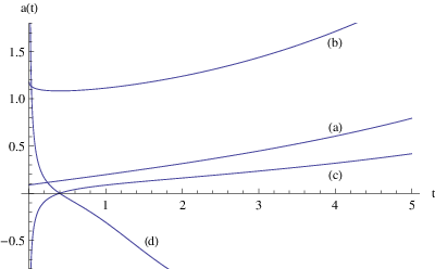
The characteristic features of the solution of (4.18) can be read from the typical and numerical solution given in the Fig. 6. The equation has been solved by the intial condition, as in the case of negative .
- •
The scale increases monotonically with almost constant velocity, . However, changes its sign at , so the expansion of the universe changes from decelerating to the accelerating one at . This implies that the dominant source of the expansion changes from the radiation to the positive dark energy at this time.
- •
It would be meaningful to see the value of at this point. We find it as
(4.21) This relation is also independent of the parameters of the theory as seen at the phase transition point above. The meaning of this fact would be discussed in the future work.
Emergence of the second horizon at
Next, we examine what happens at . In the present case of positive , is positive at any point of . As a result, the horizon represented by exists does not disappear at any time and as seen by the curve (b) in the Fig. 7. In other words, the theory is in the deconfinement phase at any time although the temperature decreases with increasing . In this sense, there is no phase transition to the confinement phase.
On the other hand, we observe that decreases from a large positive value and crosses -1/3 at an appropriate time, then decreases further and approaches to -1 for . It is interesting to see what happens in the present case after crosses . Our observation is summarized as follows.

- •
(i) There is no confinement deconfinement phase transition at this point as mentioned above. This is because of the fact that the theory for , where the radiation disappears and , is in the deconfinement phase as shown for the case. So the system should be continuing as the deconfinement phase even if the state is in the region .
- •
(ii) While the horizon () observed for smoothly varies as a horizon with positive value. On the other hand, when crosses , the value of changes its sign to positive. This implies that the second horizon, appears for . Then we could say that in the holographic sense, two theories are explicitly described by the dual 5D geometry for . Two boundaries for each horizon exist in this case, so we will find two 4D field theories on those boundaries. A similar case has been discussed in [23]. However, the two CFT would be non-interacting since they are not causal due to the two horizons between the boundaries [24]. Similar situation has been found and discussed in the case of negative [25]. On this point, we will discuss in the future work.
Instanton solution for
Up to here, we have examined the case of Lorentzian time, and we find one turning point for the case of . For , we can find a Euclidean time solution with two turning points for . Barvinsky, Kamenshchik, and Nesterev [26] have used this solution to construct a new hill-top inflation scenario. In this sense, this type of solution is very interesting, but we will discuss on this solution in the future.
5 Solution of
At the point of , takes its maximum value . The value of larger than this maximum of is realized by . So the solution of the equation solved here covers the side of larger than the case of .
In the present case, is always positive, so we can take any value of , . In any case, grows exponentially with the at enough large , where is positive and almost constant as shown in the Fig. 8. The typical solution is shown in the left of the Fig. 8. In this case, there is no turning point, so the Universe continues to expand exponentially forever.


Some important observations with respect to are summarized as follows.
- •
First, we observe that increases from to -1 with increasing time. The state is restricted to the region of , where the state is called as the phantom state since the kinetic energy is negative. How do we interpret this fact here is an open problem.
- •
As mentioned above, does not arrive at . As a result, the number of the horizon does not changes. We observe two horizons at any t. See Fig. 9

About the Connectedness of and at
As pointed out above, the solutions of and are connected at the sudden singularity, namely at the point of . The scalar curvature is divergent at this point. So it is not simple to connect the two solutions due to the singularity. As for this problem, there is an interesting approach proposed by Awad [19]. This idea is very interesting to make an inflation scenario, however, we would postpone to discuss this issue to the future work.
6 Summary and Discussion
In AdS/CFT, boundary gravity decouples from the bulk, and the boundary metric becomes nondynamical. Hence, the time-dependent scale factor in a FRW space-time on the boundary can not be determined self-consistently from the equations of motion of the bulk gravity theory, which in our case is a truncation of 10D supergravity. On the other hand, the bulk solution induces energy and momentum sourcing gravity on the boundary via the usual AdS/CFT dictionary for the metric. For example, a finite temperature state in the bulk (an AdS-Schwarzschild black hole), will induce a radiation energy density and a corresponding pressure on the boundary. Hence, in order to obtain a self-consistent holographic cosmological evolution, we need to impose the dynamics of the scale factor by hand.
In this work we proposed a way to do so by imposing the Friedmann equations for the boundary metric which relate energy density and pressures of the dual field theory to the time-development of the CFT by giving a solution for the scale factor . We hence solved the 4D boundary Einstein equations coupled to the SYM theory energy-momentum tensor and to a boundary cosmological constant . The energy momentum tensor itself is obtained from the holographic renormalization procedure in the the 5D reduction of type IIB 10D supergravity. By using the solved in this way we were able to find a time dependent 5D gravitational background, which consistently describes the time dependence of the state of SYM theory in the FRW space-time via the AdS/CFT correspondence.. The solution is characterized by two free parameters, and , the 4D cosmological constant and the dark radiation constant of the SYM fields. These two parameters control the dynamical properties of the SYM theory.
We then proceeded to analyze the phase structure of the SYM theory for different cases of these parameters. Our general finding is that negative drives the theory to a Wilson loop confinement phase. On the other hand, the dark radiation counteracts this tendency by the screening of the confinement force. Hence these competing effects lead to a confinement-deconfinement transition. The same phenomenon had been observed for the case of slowly varying already in [7]-[12].
We find that the solution for has two branches, and . These two branches arise from solving a quadratic equation for . 44 4 We should notice here that is not but it is given by and the dark radiation as shown above. Both solutions have a minimum of the scale factor , and both branches meet at this point. This point turns out to be singular since the acceleration diverges. At this point, the classical Friedmann equation breaks down, and quantum gravitational effects have to be taken into account to resolve the singularity, which is beyond the scope of this work.
The first branch itself separates into two cases depending on the sign of . For negative , the region of negative values of is covered. The Friedmann equation is then solved for hyperbolic () three-dimensional spatial topology and we find that the solution increases with time and arrives at a maximum turning point with and . After that, turns back to the singular point . An important phenomenon in this case is that, before arriving at , we find a phase transition of the SYM theory from the (Wilson loop) deconfinement to the confinement phase at a critical time . This transition happens exactly when the horizon zero in , which is present in the deconfinement phase at small , disappears. We have observed that at this transition point, the value of the ratio of the pressure to the energy density is exactly . This value is in particular independent of the two free parameters of the theory and . The meaning of this value has been discussed from the viewpoint of the Virial equilibrium. We would like to stress that the energy-momentum tensor components and (and hence also ) vary smoothly across the transition, which hence only shows in the Wilson loop potential.
In the case of , is always positive, and we can solve the Friedmann equation for any value of the spatial curvature , namely for and . In order to compare with the case of , we have first examined the case of negative curvature, . In this case, the solution increases monotonically and has no turning point. It furthermore has the following properties: First, the acceleration changes its sign from positive to negative at an appropriate time. While we find that is realized at this changing point independently of the parameters, its physical interpretation is an open question here. On the other hand, we find no phase transition at the point of since the horizon zero in remains present for all regions of . Thirdly, we noticed that a second horizon appears for , an interesting observation whose meaning we plan to investigate in a future work. Finally, for we found a Euclidean solution with two turning points. This solution has been used in [26] as an instanton solution to drive an inflation scenario. In our case such solutions exist for special values of the parameters, and . We postpone to discuss about this kind of solution related to the inflation scenario and the quantum cosmology.
For the second branch, , the solution increases monotonically with time in all cases and never has a turning point. At enough large , it expands exponentially as expected since is positive and grows . The value of increases monotonically from to -1, so at any . So the matter is in a phantom phase. We find always two horizons in this case.
Of course, the time dependence of the solutions obtained here depends on the 4D gravity model on the boundary as well as on the 5D bulk theory and the chosen solution therein. In the present case, it is constructed by the Einstein-Hilbert action with a cosmological constant and SYM theory. In general, other matter fields might be included, or the 4D Einstein equations could be modified. For example, higher order curvature terms may be needed near the ”sudden” singularity to resolve it. In this sense, some parts of the above results will be model dependent, but the chosen model, a otherwise conformal ground state in the bulk with only temperature turned on as well as the prudent choice of the standard two-derivative Einstein-Hilbert action coupled minimally to energy and momentum as well as a cosmological constant on the boundary is the simplest reasonable choice. Also, the results obtained here would be remained as useful clue when we perform the analysis of more complicated models.
Acknowledgments
The authors would like to thank M. Ishihara for useful discussions and comments. K. G thanks J. Erdmenger for encouragement.
References
- [1] J. M. Maldacena, “The Large N limit of superconformal field theories and supergravity,” Adv. Theor. Math. Phys. 2, 231 (1998) [Int. J. Theor. Phys. 38, 1113 (1999)] [hep-th/9711200].
- [2] S. S. Gubser, I. R. Klebanov and A. M. Polyakov, “Gauge theory correlators from noncritical string theory,” Phys. Lett. B 428, 105 (1998) [hep-th/9802109].
- [3] E. Witten, “Anti-de Sitter space and holography,” Adv. Theor. Math. Phys. 2, 253 (1998) [hep-th/9802150].
- [4] T. Hirayama, JHEP 0606, 013(2006) [hep-th/0602258].
- [5] K. Ghoroku M. Ishihara and A. Nakamura, “Gauge theory in de Sitter space-time from a holographic model,” Phys. Rev. D74 124020 (2006) .
- [6] K. Ghoroku M. Ishihara and A. Nakamura, “Flavor quarks in AdS4 and gauge/gravity correspondence,” Phys. Rev. D75 046005 (2007) .
- [7] J. Erdmenger, K. Ghoroku, R. Meyer, “Holographic (De)confinement Transitions in Cosmological Backgrounds ,” Phys.Rev. D84, 026004 (2011), [arXiv:1105.1776 (hep-th)] ; J. Erdmenger, K. Ghoroku, R. Meyer and I. Papadimitriou, “Holographic Cosmological Backgrounds, Wilson Loop (De)confinement and Dilaton Singularities,” Fortsch.Phys. 60 (2012) 991-997 [arXiv:1205.0677 (hep-th)]
- [8] P. Binetruy, C. Deffayet, U. Ellwanger and D. Langlois, “Brane cosmological evolution in a bulk with cosmological constant,” Phys.Lett. B477 (2000) 285-291,[hep-th/9910219]
- [9] D. Langlois, “Brane cosmological perturbations,” Phys .Rev. D62 126012 (2000) [hep-th/0005025] D. Langlois and L. Sorbo “Bulk gravitons from a cosmological brane,” Phys .Rev. D68 084006 (2003) [hep-th/0306281]
- [10] T. Shiromizu, K. Maeda and M, Sasaki, “The Einstein equation on the 3-brane world,” Phys. Rev. D62, 024012 (2000) [gr-qc/9910076]
- [11] M, Sasaki, T. Shiromizu and K. Maeda, “Gravity, stability and energy conservation on the Randall-Sundrum brane world,” Phys. Rev. D62, 024008 (2000) [hep-th/9912233]; K. Maeda, S. Mizuno and T. Torii, “Effective gravitational equations on brane world with induced gravity,” Phys. Rev. D68, 024033 (2003) [gr-qc/0303039];
- [12] K. Ghoroku and A. Nakamura, “Holographic Friedmann equation and N=4 supersymmetric Yang-Mills theory,” Phys. Rev. D87 063507 (2013) [arXiv:1212.2304 (hep-th)]
- [13] K. Ghoroku, M. Ishihara, M. Tachibana, and F. Toyota, “Chiral symmetry of SYM theory in hyperbolic space at finite temperature,” Phys. Rev. D92 026011 (2015) [arXiv:1502.04811(hep-th)]
- [14] C. Fefferman and C. Robin Graham, ‘Conformal Invariants’, in Elie Cartan et les Mathématiques d’aujourd’hui (Astérisque, 1985) 95.
- [15] S. de Haro, S. N. Solodukhin and K. Skenderis, Commun. Math. Phys. 217, 595 (2001) [hep-th/0002230].
- [16] Massimo Bianchi, Daniel Z. Freedman, Kostas Skenderis, Nucl.Phys. B631 (2002) 159-194, [hep-th/0112119].
- [17] Pantelis S. Apostolopoulos, George Siopsis, Nikolaos Tetradis, ”Cosmology from an AdS Schwarzschild black hole via holography”, Phys.Rev.Lett.102:151301 (2009) [arXiv:0809.3505 (hep-th)].
- [18] Kiri] Elias Kiritsis, Vasilis Niarchos, ”Josephson Junctions and AdS/CFT Networks”, JHEP07(2011)112, [arXiv:1105.6100 [hep-th]].
- [19] A. Awad, ”Weyl Anomaly and Initial Singularity Crossing”, Phys. Rev. D 93, 084006 (2016), arXiv:1512.06405[hep-th]
- [20] G. W. Gibbons, M. B. Green and M. J. Perry, Phys.Lett. B370 (1996) 37-44, [hep-th/9511080].
- [21] A. Kehagias and K. Sfetsos, Phys. Lett. B 456, 22(1999) [hep-th/9903109].
- [22] H. Liu and A.A. Tseytlin [hep-th/9903091].
- [23] Juan M. Maldacena, ”Eternal Black Holes in AdS”, JHEP 0304 (2003) 021, [ arXiv:hep-th/0106112].
- [24] Ali Mollabashi, Noburo Shiba, Tadashi Takayanagi, ” Entanglement between Two Interacting CFTs and Generalized Holographic Entanglement Entropy2, JHEP04(2014)185, [ arXiv:1403.1393 [hep-th]].
- [25] K. Ghoroku, M. Ishihara, and A. Nakamura, “AdS5 with two boundaries and holography of N=4 SYM theory,” Phys. Rev. D89 066009 (2014) [arXiv:1310.2007 (hep-th)]
- [26] A. O. Barvinsky, A. Yu. Kamenshchik, D.V. Nesterev, arXiv:1510.06858[hep-th]