Using a quantum work meter to test non-equilibrium fluctuation theorems
Abstract
Work is an essential concept in classical thermodynamics, and in the quantum regime, where the notion of a trajectory is not available, its definition is not trivial. For driven (but otherwise isolated) quantum systems, work can be defined as a random variable, associated with the change in the internal energy. The probability for the different values of work captures essential information describing the behaviour of the system, both in and out of thermal equilibrium. In fact, the work probability distribution is at the core of “fluctuation theorems” in quantum thermodynamics. Here we present the design and implementation of a quantum work meter operating on an ensemble of cold atoms, which are controlled by an atom chip. Our device not only directly measures work but also directly samples its probability distribution. We demonstrate the operation of this new tool and use it to verify the validity of the quantum Jarzynksi identity.
I Introduction
Classical fluctuation theorems establish surprising relations between non-equilibrium and equilibrium concepts. In particular, the work performed on a system during non-equilibrium processes is connected with key concepts of equilibrium thermodynamics, such as the free-energy [1, 2]. These relations have been verified in various experiments involving microscopic thermodynamic systems [3, 4, 5]. Recent advances in quantum technologies enable the control of small quantum systems that can be manipulated far from the regime where the usual thermodynamical laws are obeyed. This triggered the development of the rapidly growing field of non-equilibrium quantum thermodynamics [6, 7, 8, 9].
When quantum fluctuations dominate, defining and measuring work and heat, two central concepts in classical thermodynamics, is non-trivial. For driven, but otherwise isolated, quantum systems, work is a random variable associated with the change in the internal energy [10], as the first law of thermodynamics indicates. Thus, the commonly accepted definition of quantum work requires a two-time measurement strategy, which consists of performing two projective energy measurements, one at the beginning and the other at the end of the process. Then, work is associated with the measured energy difference. However, implementing the two-time measurement is experimentally difficult [11, 12] due to the fact that the two projective measurements are unavoidably disruptive (see Ref. [13] for an ion trap implementation). Alternative methods to evaluate the work probability distribution that rely on the direct estimation of its Fourier transform were also proposed in Refs. [14, 15] and later implemented in NMR experiments [16].
In this paper we present the design and the experimental implementation of a “quantum work meter” (QWM)
operating on an ensemble of cold atoms, combining the idea presented in Ref. [17] and the
experimental setup used in Ref. [18].
Our QWM is conceptually different from previous work-measurement devices.
Its main advantage is that the QWM efficiently samples , which is a direct observable in the experiment.
Namely, our QWM not only directly measures work but also directly samples its probability
distribution [i.e. the outcome is obtained with probability ]. As the work probability distribution
plays a central role in the fluctuation theorems of non-equilibrium quantum thermodynamics,
the QWM is an ideal tool to test their validity. In particular,
we use it to verify the Jarzynski identity [1, 19, 20, 21, 10].
II Results
Work measurement and the QWM. A QWM is an apparatus that measures the work performed on a driven quantum system whose Hamiltonian varies from an initial to a final with eigenvalues and , respectively. For an isolated system , with a -dimensional space of states, the number of different values of work is bounded by . Therefore, the pointer of the QWM has distinct positions (one for each value of ). The QWM presented here enables us to choose and (fixing the possible values of ) and to vary the intermediate driving (inducing different evolution operators denoted as ). In this way, we vary the probability , which depends on the intermediate driving .
By sampling , we use the QWM to verify a fundamental result in non-equilibrium quantum thermodynamics: the Jarzynski identity. This identity states that for any initial state with populations identical to the ones associated to a thermal Gibbs state and for any distribution , the linear combination , where is the inverse temperature of the system, is an equilibrium property (rather than a non-equilibrium one). The Jarzynski identity (see the Supplementary Note 1) reads
| (1) |
where is the free energy difference between the thermal states associated with the Hamiltonians and . In the absence of degeneracies, this implies that the vector formed by the measured probabilities belongs to a dimensional hyperplane: the “Jarzynski manifold” [as shown in the Supplementary Note 1, further constraints restrict this dimensionality to ]. With the QWM we measure for different driving fields showing that all probability vectors belong to the same manifold. By characterising this manifold, we not only verify the identity but also independently estimate the free energy difference [1, 3, 4, 5].
The work distribution sampled by the QWM [19, 20, 21, 10] is:
| (2) |
Thus, is the probability density of finding the
energy difference after a
measurement of followed by an intermediate driving
and a final measurement of . This is
indeed the case if is the probability of obtaining
when measuring and is
the probability of obtaining when
measuring given that was detected at the beginning.
Equation (3) defines a probability density that is independent of the initial
coherences in the energy basis. For the
discrete values of
we will use to denote the
probability (not the density) of each .
The concept on which our QWM is based was first discussed in Refs. [17, 22], where it was noticed
that the work done on , can be detected by performing a generalised quantum measurement, which enables the
number of outcomes to be larger than . This can be done by entangling
with an ancilla that stores a coherent record of .
Then a standard measurement on can reveal . Similar strategies have been later studied and extended to other
contexts in Refs. [22, 23, 24].

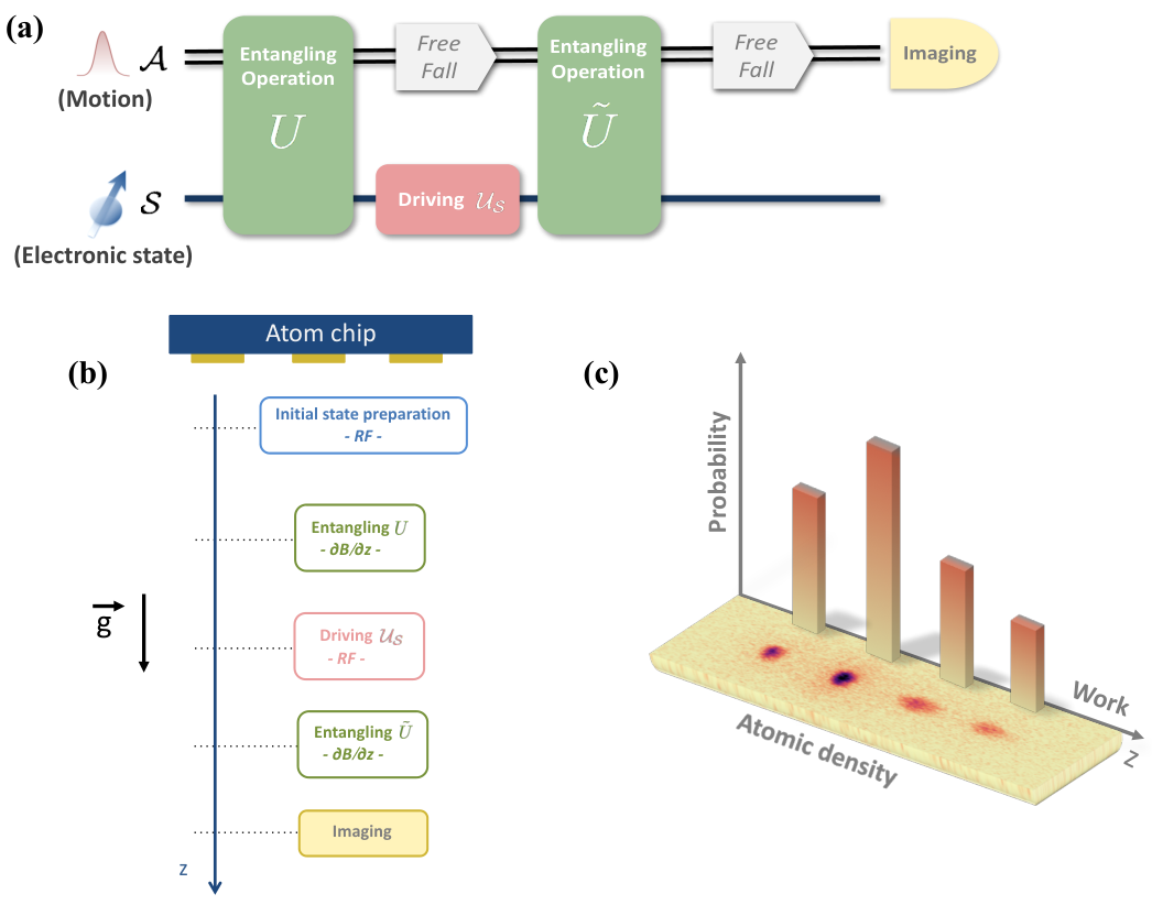
Design and operation of the QWM. A pictorial representation of the protocol we follow to operate the QWM is shown in Fig. 1a. The QWM is designed to measure the work done on a system whose Hamiltonian changes from to and which is subjected to a driving in between. We couple to a continuous variable system and use to denote its position (the generator of translations along the momentum ). A coherent record of is created by an “entangling interaction” between and that must take place before and after the driving . The unitary operators representing these interactions are: and , where is a coupling parameter. Thus, and respectively translate along by a displacement proportional to and . Then, as shown in detail in the Supplementary Note 3, the final measurement of on yields a random result whose distribution is a smeared version of the true work distribution defined in Eq. (3). In fact, outcome is obtained with a probability density , where the window function is fixed by , the initial state of [thus, by localising we improve the accuracy in the estimation of ].
A “universal” QWM is an
apparatus which can measure
and sample for any possible
choice of and . To build it, we
need enough control to enforce the
entangling operators and for
any choice of and .
Remarkably, this is achieved for a -level system
by the atom chip implementation we
describe below.
| (JI) | (PF) | (JI) | (PF) | |
|---|---|---|---|---|
Experimental implementation of the QWM. To describe our QWM we should identify the physical systems representing and , the way in which and can be chosen, and how the associated and are implemented. In our experiment we represent by the subspace associated with the Zeeman sublevels and of a 87Rb atom that, as in Ref. [18], behaves as a two-level system (see below). The motional degree of freedom of the atom plays the role of .
A key element of the QWM presented here is the atom chip [25], which efficiently entangles the internal and motional degrees of freedom of an atom just m away from the chip surface, through short and strong Stern-Gerlach type magnetic gradient pulses. These pulses are generated using a -current-carrying-wire setup on the chip surface (described in Ref. [26] and Methods). A gradient pulse along the direction with amplitude and duration , induces a momentum kick on an atom in the state (, where and are, respectively, the Bohr magneton and the Landé factor [18]). The evolution of the state of the atom induced by such a pulse is described by the unitary operator , where the operator . This physical operation translates along the momentum by a displacement (notice that the operator defines the magnetic dipole moment of the atom since ). As described below, we apply two gradient pulses with different amplitudes ( and ) and different durations ( and ). Thus, defining and , and implement the required entangling operation and , respectively. In this implementation is consequently replaced by and , enforcing . The momentum kicks induced by both pulses are controlled in the experiment, and consequently, by fixing their ratio, we can simulate an arbitrary system with initial and final Hamiltonians and which are characterised by having the same ratio. Finally, let us note that the two pulses utilise and with opposite signs to ensure that the sequence creates a record of work corresponding to .
To achieve universality we only need to be able to fix the energy splitting and of and , as well as their eigenbasis. The traces of and (the sum of their eigenvalues) do not affect but only add a constant to all values of . As arbitrary and can be simulated and any change of basis can be absorbed into , we conclude that our atom chip QWM can sample for an arbitrary 2-level system and is thus universal.
The 87Rb atoms are magnetically trapped in state and evaporatively cooled to a Bose-Einstein condensation (BEC). The BEC is released from the trap and a radio-frequency (RF) pulse is used to prepare a superposition of and . A strong homogeneous magnetic field (created by external coils) suppresses the transitions taking into the state (due to the non-linear Zeeman effect [18]). The initial populations ( and ) are chosen so that . The initial motional state is a wave-packet localised in position and momentum.
It should be noted that the initial internal state of the atom, while having the same populations as defined by the temperature of a thermal state, is still a pure state. However, the quantum coherences of this initial state do not affect the results of the QWM. As explained in the Supplementary Note 3, the contribution of the initial coherences to the final probability is multiplied by the overlap between the motional states of the atom associated with the different values of work. Thus, when the atomic clouds associated with the different work values are well separated, the effect of initial coherences is negligible. In this regime, our experiment gives the same result as the one we would obtain by preparing an initial thermal state (with no coherences). The study of the importance of the initial coherences in the definition of work is an interesting topic in itself, which is beyond the scope of our paper (see, for example, Ref. [27, 28, 29, 24, 30]).
The experimental sequence, presented in Fig. 1b, is: i) prepare the initial state and release the cloud (which then freely falls along , the direction of gravity), ii) apply the magnetic gradient along , iii) apply the driving by exposing the atoms to a RF field resonant with the Zeeman splitting induced by the homogeneous bias field, iv) apply the gradient , v) obtain an image of the four clouds after a time-of-flight and count the number of atoms in each cloud. More details of the experiment can be found in Methods and the Supplementary Note 3. For the experimental demonstration presented here we set the ratio between the measured momentum kicks induced by the two pulses to . Hence, our realisation of the QWM samples the work distribution of a simulated system in which the energy splitting is reduced to of its original value, from to , while driven by .
Fig. 1c shows a typical image
obtained by the QWM. Four clouds are
visible.
From the positions of
the center of each cloud, , we infer
the total momentum shift, ,
induced by the pulses on that cloud
(we take into account both the
free fall and the kicks induced by the pulses, see the Supplementary Note 3).
Then, we obtain the corresponding value of work
as ( is
proportional to , whose value, together with
the experimental results, determine the work ).
Furthermore, the probability for each is directly measured
by the number of atoms in each cloud.
Notably, this experiment determines the entire distribution
in a single shot.
Testing the Jarzynski identity. We repeat the experiment fixing the timing, duration and pulse strength. We consider three initial ’s and vary the intermediate driving by changing the duration of the RF field. In this way, we obtain many sets of probability distributions, each of which defines a 3D–vector (as there are three independent probabilities). When we represent all these vectors in the same 3D-plot, we see that they all belong to the same –dependent manifold. Fig. 2a shows that this manifold is a –dependent line (the dimensionality of this “Jarzynski manifold” is , which in this case equals ).
Using the measured work probabilities we calculate the exponential average of the work for each driving field. Fig. 2b displays the value of as a function of the duration of the intermediate RF field, that parametrises . As established by the Jarzynski identity, is independent of the driving field and only depends on . The horizontal lines in Fig. 2b are the theoretically predicted values of , obtained from a direct calculation (with its own theoretical uncertainty, due to the error in the estimation of ). This calculation simply involves computing the initial and final partition functions, respectively denoted as and , and using the identity . We find that, as the Jarzynski identity establishes, . From Fig. 2b one can notice that the largest errors in the estimation of appear for . In this case, for two values of and, therefore, the relative error in the atom number estimation is large, inducing a larger error in the estimation of .
In Table 1 we compare
measured and estimated values of
. The uncertainty in the estimation of
and is close to
10%, which is enough to distinguish the three values of .
On the other hand, in the case of , there is a significant
overlap in the measured values which does not allow to properly distinguish between the three
different cases due to the error in the estimation of .
III Discussion
We presented and implemented
a QWM, a new device directly sampling
the work distribution on an ensemble of
cold atoms. Our QWM can be used to simulate
the behaviour of an arbitrary -level system.
We implemented it with an atom chip and verified the
Jarzynski identity over a wide range of non-equilibrium processes. This is the first experiment,
and so far the only one, directly sampling
offering advantages and
different perspectives over previous work measurement schemes.
Remarkably, in this cold atom experiment, the QWM
extracts full statistical information
about the work distribution in a single shot.
IV Methods
Initial state preparation. After preparing the BEC,
a homogeneous magnetic field of G (, where is Planck’s constant) is used to
push the transition to out of resonance by
kHz due to the
non-linear Zeeman effect, which is larger than the power
broadened driving RF field of . This ensures that the atoms
behave as -level systems.
The BEC is released from the trap and a RF pulse is used
to prepare a superposition of
and . By varying the relative populations we consider three different pseudo-thermal
states.
The initial motional state is a wave packet ,
well localised at m
from the chip
and momentum .
Entangling operations and measurement. An
inhomogeneous magnetic field is used to couple spin and motional
degrees of freedom.
This is generated by a current A in the 3-wire setup
during a time .
The three parallel gold wires lie on the direction
of the chip surface (Fig. 1.b). They
are mm long, m wide and m
thick. Their centers are at m
and the same current run through them in
alternating directions (, respectively),
creating a D quadrupole field at m
below the chip.
After a time of flight of ms the atoms are at
. At this point the
first gradient pulse implements :
s with an amplitude of G/mm,
such that the momentum kick is along .
Then, after 3.1 ms the atoms are at mm
and the second gradient pulse implements :
s,
G/mm, such that the momentum
kick is along . The relative strengths of the
spin-dependent forces sets the energy splitting of
the Hamiltonians which in this case is on average
(this is the measured value, that takes into account
fluctuations in the initial
position of the cloud and in the gradient pulses).
In between the entangling operation is applied
with a RF pulse.
Finally, an image of the atomic clouds is obtained after a
time-of-flight of ms after the nd gradient
(the clouds are centered around mm). The
position and
number of atoms of each cloud is determined.
The momentum shifts of each cloud (that codifies the value of )
are obtained from the difference in positions between the
clouds, that follow approximately classical trajectories (see Supplementary Note 3).
Uncertainties.
The main source of position error is the initial distance of the cloud from the atom chip, whose uncertainty is .
This error is later translated to momentum uncertainty, since the field gradients are position dependent.
The field gradients have a
fractional uncertainty of due to current fluctuations [18].
The central position of each
cloud is estimated by fitting a Gaussian profile.
Each work probability is estimated as a normalised sum of the measured
optical density in a relevant region around the cloud,
introducing probability uncertainty (due to atom numbers uncertainty). Our optical resolution also induces an error in the determination of the position for each cloud.
We perform three different runs for each combination of initial
state population ratios and intermediate driving
and use the average values of position and probability.
This gives us a position uncertainty of and a probability uncertainty
of (standard error).
Acknowledgments.
FC, AJR and JPP acknowledge financial support from ANPCyT (PICT 2013-0621 and PICT 2014-3711), CONICET
and UBACyT. YM and RF gratefully acknowledge funding by the
Israel Science Foundation, the EC Matter-Wave consortium
[FP7-ICT-601180],
and the German DFG through the DIP program [FO703/2-1]. SM acknowledges
financial support by the Foundation for Fundamental Research on Matter (FOM),
which is part of the Netherlands Organisation for Scientific Research (NWO).
We also thank the BGU nano-fabrication team for
making available the high quality chip, and Zina Binstock
for helping with the electronics.
References
- [1] Jarzynski, C. Nonequilibrium equality for free energy differences. Physical Review Letters 78, 2690–2693 (1997).
- [2] Crooks, G. E. Entropy production fluctuation theorem and the nonequilibrium work relation for free energy differences. Physical Review E 60, 2721–2726 (1999).
- [3] Hummer, G. & Szabo, A. Free energy reconstruction from nonequilibrium single-molecule pulling experiments. Proceedings of the National Academy of Sciences 98, 3658–3661 (2001).
- [4] Liphardt, J., Dumont, S., Smith, S. B., Tinoco, I. & Bustamante, C. Equilibrium information from nonequilibrium measurements in an experimental test of jarzynski’s equality. Science 296, 1832–1835 (2002).
- [5] Collin, D. et al. Verification of the crooks fluctuation theorem and recovery of rna folding free energies. Nature 437, 231–234 (2005).
- [6] Esposito, M., Harbola, U. & Mukamel, S. Nonequilibrium fluctuations, fluctuation theorems, and counting statistics in quantum systems. Reviews of Modern Physics 81, 1665–1702 (2009).
- [7] Campisi, M., Hänggi, P. & Talkner, P. Colloquium: Quantum fluctuation relations: Foundations and applications. Reviews of Modern Physics 83, 771–791 (2011).
- [8] Seifert, U. Stochastic thermodynamics, fluctuation theorems and molecular machines. Reports on Progress in Physics 75, 126001 (2012).
- [9] Goold, J., Huber, M., Riera, A., del Rio, L. & Skrzypczyk, P. The role of quantum information in thermodynamics—a topical review. Journal of Physics A: Mathematical and Theoretical 49, 143001 (2016).
- [10] Talkner, P., Lutz, E. & Hänggi, P. Fluctuation theorems: Work is not an observable. Physical Review E 75, 050102 (2007).
- [11] Huber, G., Schmidt-Kaler, F., Deffner, S. & Lutz, E. Employing trapped cold ions to verify the quantum jarzynski equality. Physical Review Letters 101, 070403 (2008).
- [12] Watanabe, G., Venkatesh, B. P. & Talkner, P. Generalized energy measurements and modified transient quantum fluctuation theorems. Physical Review E 89, 052116 (2014).
- [13] An, S. et al. Experimental test of the quantum jarzynski equality with a trapped-ion system. Nature Physics 11, 193–199 (2015).
- [14] Mazzola, L., De Chiara, G. & Paternostro, M. Measuring the characteristic function of the work distribution. Physical Review Letters 110, 230602 (2013).
- [15] Dorner, R. et al. Extracting quantum work statistics and fluctuation theorems by single-qubit interferometry. Physical Review Letters 110, 230601 (2013).
- [16] Batalhão, T. B. et al. Experimental reconstruction of work distribution and study of fluctuation relations in a closed quantum system. Physical Review Letters 113, 140601 (2014).
- [17] Roncaglia, A. J., Cerisola, F. & Paz, J. P. Work measurement as a generalized quantum measurement. Physical Review Letters 113, 250601 (2014).
- [18] Machluf, S., Japha, Y. & Folman, R. Coherent stern–gerlach momentum splitting on an atom chip. Nature Communications 4, 2424 (2013).
- [19] Tasaki, H. Jarzynski relations for quantum systems and some applications. Preprint at https://arxiv.org/abs/cond-mat/0009244 (2000).
- [20] Kurchan, J. A quantum fluctuation theorem. Preprint at https://arxiv.org/abs/cond-mat/0007360 (2000).
- [21] Mukamel, S. Quantum extension of the jarzynski relation: analogy with stochastic dephasing. Physical Review Letters 90, 170604 (2003).
- [22] De Chiara, G., Roncaglia, A. J. & Paz, J. P. Measuring work and heat in ultracold quantum gases. New Journal of Physics 17, 035004 (2015).
- [23] Talkner, P. & Hänggi, P. Aspects of quantum work. Physical Review E 93, 022131 (2016).
- [24] Solinas, S., Miller, H. J. D. & Anders, J. Measurement-dependent corrections to work distributions arising from quantum coherences. Preprint at https://arxiv.org/abs/1705.10296 (2017).
- [25] Keil, M. et al. Fifteen years of cold matter on the atom chip: promise, realizations, and prospects. Journal of Modern Optics 63, 1840–1885 (2016).
- [26] Margalit, Y. et al. A self-interfering clock as a “which path” witness. Science 349, 1205–1208 (2015).
- [27] Solinas, P. & Gasparinetti, S. Full distribution of work done on a quantum system for arbitrary initial states. Physical Review E 92, 042150 (2015).
- [28] Kammerlander, P. & Anders, J. Coherence and measurement in quantum thermodynamics. Scientific reports 6, 22174 (2016).
- [29] Perarnau-Llobet, M., Bäumer, E., Hovhannisyan, K. V., Huber, M. & Acin, A. No-go theorem for the characterization of work fluctuations in coherent quantum systems. Physical Review Letters 118, 070601 (2017).
- [30] Sampaio, R., Suomela, S., Ala-Nissila, T., Anders, J. & Philbin, T. G. The impossible quantum work distribution. Preprint at https://arxiv.org/abs/1707.06159 (2017).
Appendix A Supplementary Material.
Supplementary Note 1 - Jarzynski identity and quantum work measurement
Work is the energy variation induced on a system by a certain driving (the system is otherwise isolated). Suppose that the Hamiltonian of changes from an initially to a final and that the system is driven by a certain unitary operator in between. We denote the eigenvalues and eigenvectors of as and (where labels different eigenstates with the same energy). In turn the eigenvalues and eigenvectors of are denoted as and (again, labels states with the same energy ). Suppose that we measure the energy at the initial and final times. The work probability distribution is nothing but the probability density to obtain a value as the difference between the results of the two energy measurements. This can obviously be computed as
| (3) |
where is the probability of initially measuring energy and is the probability of measuring energy at the end of the driving given that was detected at the beginning. If the initial state of is , the above probabilities can be simply written in terms of the projectors and . Thus,
| (4) |
Jarzynski identity follows immediately from the above definition of the work probability distribution. In fact, if we compute the exponential average of the work, we get
| (5) | |||||
If the initial state is thermal, then (where is the partition function with being the degeneracy of level ). Then, we can replace and perform the summation over the label by noticing that . In this way we obtain
where the partition function of the final Hamiltonian is , with the degeneracy of level . The final step that leads to the Jarzynski identity is simply to notice that for a Gibbs state we have . Thus, the average exponential work becomes independent of the intermediate driving process and turns out to be determined by equilibrium properties. Thus, .
When has a finite dimensional Hilbert space, can only take discrete values. In this case, instead of using the probability density we use directly the probability for each value of . Thus, we can arrange as a vector with components. Taking into account the normalisation condition, the vector of independent probabilities is dimensional. In turn, being the Jarzynski identity a linear equation in terms of it constraints the probability vector to belong to a dimensional hyperplane. But, of course, there are further constrains reducing the number of independent probabilities. The simplest way to obtain this number is to go back to the definition of in Supplementary Equation (3) and count the number of free parameters we have. In this equation, the probabilities are fixed by the initial state. Then, the number of independent probabilities is determined by the number of independent parameters in . For the non-degenerate case we consider here (where all the values of work are different), the calculation is simple. In fact, the coefficients form a doubly stochastic matrix (since they are all positive numbers such that ). For such square matrix of dimension , there is always free parameters. Indeed, this is the dimensionality of the manifold of where the probability vector lies. Jarzynski identity establishes that this manifold is a -dependent hyperplane (a line in our case, where ).
Supplementary Note 2 - Work measurement as a POVM
Let us consider a system with a -dimensional space of states and show, in a simple way, that the work measurement can be viewed as a generalised quantum measurement. For this, we start by writing the probability for a given value of work as
| (6) |
Using the formula for the transition probability, we find that
| (7) |
where
| (8) |
It is simple to verify that the operators expand the identity as and that they are positive semi-definite (i.e., that for any state we have ). Therefore, the operators define a positive operator valued measure (POVM), which is the most general type of measurement one can perform in quantum mechanics. Therefore, work can be measured in the same way as any POVM can: A powerful result (Neumark’s theorem) establishes that any POVM can be realised by coupling the system with an ancillary system and then performing a standard projective measurement on . This measurement can be performed at a single time. Thus, surprisingly, the two-time work measurement strategy can be replaced by a single-time strategy (which is the basic idea exploited by our QWM). In the following section we show how one can construct an approximation for that ideal apparatus, that we call Quantum Work Meter (QWM).
Supplementary Note 3 - Probability distribution for the outcome of a QWM
Here we compute the probability distribution for the result of the measurement of the auxiliary register of a general Quantum Work Meter. The protocol defining the apparatus is shown in Figure 1 of the main text. A system is coupled to an ancillary one . This ancilla is a continuous variable system (of course this can be relaxed). The system and the ancilla are subject to the following evolution: an entangling interaction is applied (which correlates and ), the evolution is applied on the system , a second entangling interaction is applied. Finally, after this sequence is measured. The initial state of the system formed by will be assumed to be a product state. For simplicity, we first assume that the states are pure and denote them as (the state of ) and (the state of ). We will later generalise the result for an initial state which is a tensor product of arbitrarily mixed states. After the sequence of operations we described above, the total final state is:
The nature of the two entangling operations, that was discussed in the main text, is such that they both induce translations of which depend on the state of . More specifically, and , where we use to denote the generator of translations of along a certain variable . Using this, it is simple to rewrite the final state as
In this equation the displacement operators act on the states of and are defined as .
The interpretation of the above equation is simple: After the sequence of operations, and become entangled in such a way that a record of is stored in . The states are “flag states” associated with the different values of work. When these states are orthogonal, they can be unambiguously distinguished and the value of work can be retrieved. Below, we will consider a more realistic scenario where the initial state of is a localised coherent state. In that case, the flag states are displaced coherent states (which are simply translated along the variable direction by an amount that is proportional to ). These states are not strictly orthogonal, but have a finite overlap. This induces an error in the work estimation protocol. However, the error can be exponentially reduced by simply increasing the interaction strength (as the overlap exponentially decreases with ).
From the above expression it is simple to obtain the quantum state of by computing its reduced density matrix (which is obtained from the total state by tracing out the system ). Thus,
| (9) |
This expression can be generalised to the case where the initial states of and are initially mixed. In fact, if and respectively denote the initial density matrices of and , the final state of is
| (10) |
From the above equation we obtain the probability density for detecting the value in a measurement of . Thus,
| (11) |
The contribution of the diagonal () and off-diagonal () terms play a different role in the above expression. In fact, it is simple to show that the diagonal contribution is a smeared version of the true work distribution. Thus,
| (12) |
where the window function is
| (13) |
Therefore, the off-diagonal terms of are responsible for the error in the work estimation and should be made small for it to be accurate. It is simple to show that if the momentum wave function of the initial state is a Gaussian with a momentum dispersion ( is the position dispersion), then the off-diagonal terms are bounded by:
Thus, by increasing (the interaction strength) or (the position dispersion of the initial state) we exponentially reduce the error in the work estimation. It is worth noting that by increasing we reduce the momentum uncertainty and localise the initial state in momentum. Naturally, the method becomes precise when the initial localisation in momentum is much smaller than the difference between the first momentum kicks (which is fixed by the product ). When these conditions are satisfied, the off-diagonal terms can be neglected and the probability density to detect is
where the window function is defined as (which, for a coherent state is simply ).
QWM using an atom chip
Here we consider the implementation of the QWM using a cloud of atoms in a chip. As described in the main text, is the pseudo spin 1/2 associated with the , hyperfine states of a atom (which, as discussed in the main text, behaves as a two level atom). is encoded in the motional degrees of freedom of each atom. There are two subtle differences between the ideal protocol for a QWM described in the previous section and the implementation in an atom chip. The first different concerns the final measurement. Thus, in the previous section we computed the probability for a final momentum measurement but in the real experiment we are forced to measure the atomic position by taking an image of the atomic clouds. Therefore we will show below that the position measurement enables us to determine work and sample . The second difference is that in the real experiment we should take into account the fact that the ancilla evolves during the whole process because the atoms actually move (they freely fall along the vertical direction). Thus, the real protocol describing the experiment is shown in Fig. 3.
Let us now analyse this process. We can first neglect the free fall taking place between the two entangling operations (we take this into account later) and assume the initial state of is a coherent state localised around initial values of position and momentum which we arbitrarily take as and . We denote this state as . The calculation presented in the above section should be slightly modified. In this case the flag states are . Taking into account that (where is the duration of the free-fall, is the mass of the atoms, and the gravity acceleration) we can easily compute the expectation value of the position for each flag state (as well as the corresponding position dispersion). In fact, we have
| (14) |
Therefore, we can notice that by measuring the final position of the atoms we can infer the value of the momentum before the fall and thus acquire information about work . In fact, the difference between the positions of the clouds is proportional to the difference in the values of work. The price we have to pay, is that the spread of the wave packets increases during the free-fall.
In a more realistic description of the experiment, we need to include also the free fall between the entangling gates ( in the Supplementary Figure 3). It is easy to verify that since (where is the duration of the free fall), then . Thus, the first term is the usual entangling operation and the last term is just a phase depending on the value of the energy. In turn, the second term is an entangling operation where the atom is displaced along position (instead of momentum) depending on the state of . In summary, the free-fall in between the entangling gates simply induces an extra translation of the atoms by an amount that depends on the final value of the energy.
Finally, we show in the Supplementary Figure 4 the distribution probability that we obtain in each experiment. In the plots we show the projections of the Jarzynski manifold, that appears in Fig. 2 (a) of the main text, onto the different axes.