Loom: Exploiting Weight and Activation Precisions to Accelerate Convolutional Neural Networks
Abstract.
Loom (LM), a hardware inference accelerator for Convolutional Neural Networks (CNNs) is presented. In LM every bit of data precision that can be saved translates to proportional performance gains. Specifically, for convolutional layers LM’s execution time scales inversely proportionally with the precisions of both weights and activations. For fully-connected layers LM’s performance scales inversely proportionally with the precision of the weights. LM targets area- and bandwidth-constrained System-on-a-Chip designs such as those found on mobile devices that cannot afford the multi-megabyte buffers that would be needed to store each layer on-chip. Accordingly, given a data bandwidth budget, LM boosts energy efficiency and performance over an equivalent bit-parallel accelerator. For both weights and activations LM can exploit profile-derived per layer precisions. However, at runtime LM further trims activation precisions at a much smaller than a layer granularity. Moreover, it can naturally exploit weight precision variability at a smaller granularity than a layer. On average, across several image classification CNNs and for a configuration that can perform the equivalent of 128 multiply-accumulate operations per cycle LM outperforms a state-of-the-art bit-parallel accelerator (1) by without any loss in accuracy while being more energy efficient. LM can trade-off accuracy for additional improvements in execution performance and energy efficiency and compares favorably to an accelerator that targeted only activation precisions. We also study 2- and 4-bit LLM variants and find the the 2-bit per cycle variant is the most energy efficient.
1. Introduction
Deep neural networks (DNNs) have become the state-of-the-art technique in many recognition tasks such as object (2) and speech recognition (3). Given their many applications and high computation and memory demands, DNNs are prime candidates for hardware acceleration. While a few different types of DNNs exist, Convolutional Neural Networks (CNNs) in particular dominate applications where the input is an image or video. Devices executing such CNNs will be required to perform mostly if not only inference. An example is computational photography where machine learning has shown great promise in replacing classical algorithms (4).
We present Loom (LM), a hardware accelerator for inference with CNNs targeting embedded systems where reducing the amount of data transfered per memory connection, be it an external or internal one, is paramount. Specifically, given a memory bandwidth budget LM’s goal is to boost performance and energy efficiency compared to a state-of-the-art data-parallel accelerator. LM exploits the precision requirement variability of CNNs to reduce the memory footprint, increase bandwidth utilization, and to deliver performance which scales inversely proportional with precision for both convolutional (CVLs) and fully-connected (FCLs) layers. Ideally, compared to using a fixed precision of 16 bits, LM achieves a speedup of and for CVLs and FCLs where and are the precisions of weights and activations, respectively. LM also reduces the number of weight and activation bits read by and . To deliver these benefits LM processes both activations and weights bit-serially while compensating for the loss in computation bandwidth by exploiting parallelism. Judicious reuse of activations and weights enables LM to improve performance and energy efficiency over conventional bit-parallel designs without requiring a wider memory interface. For both weights and activations LM utilizes profile-derived per layer precisions. For activations, LM further trims their precision at a much finer granularity at runtime utilizing the approach of Lascorz et al. (5). By exploiting precision LM delivers benefits for all activations and weights regardless of whether they are ineffectual or not.
We evaluate LM on an SoC and compare against a bit-parallel fixed-precision accelerator (DPNN) over a set of image classification CNNs. For a configuration that is sized to match the peak computation bandwidth of a bit-parallel accelerator that can perform at peak 128 multiply-accumulate operations per cycle, on average LM yields a speedup of , , and over DPNN for the convolutional, fully-connected, and all layers, respectively. The energy efficiency of LM over DPNN is , and for the aforementioned layers, respectively. LM enables trading off accuracy for additional improvements in performance and energy efficiency. For example, accepting a 1% relative loss in accuracy, LM yields higher performance and more energy efficiency than DPNN. We also perform a sensitivity study varying the equivalent peak compute bandwidth and the number of bits that LM processes per cycle. LM scales well up up to a configuration equivalent to 256 multiply-accumulate operations per cycle and that a 2-bit per cycle design achieves the best energy efficiency albeit not the best performance.
The rest of this document is organized as follows: Section 2 illustrates the key concepts behind LM via an example. Section 3 presents the DPNN and Loom architectures. The evaluation methodology and experimental results are presented in Section 4. Section 5 reviews related work, and Section 6 concludes.
2. Loom: A Simplified Example
This section explains how LM would process CVLs and FCLs on an example using 2-bit activations and weights.
Conventional Bit-Parallel Processing: Figure 1a shows a bit-parallel processing engine which multiplies two input activations with two weights generating a single 2-bit output activation per cycle. The engine can process two new 2-bit weights and/or activations per cycle a throughput of two products per cycle.
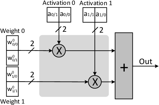
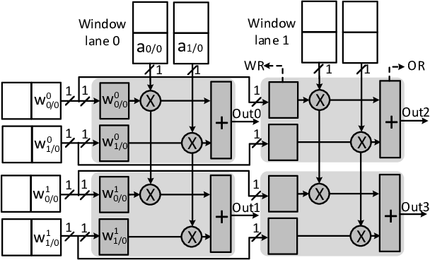
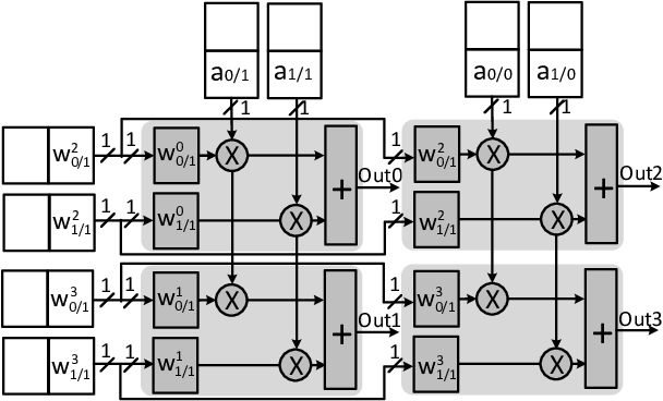
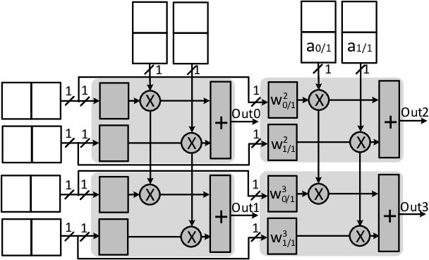
Loom’s Approach: Figure 1b shows an equivalent LM engine which matches the bit-parallel engine’s throughput by producing 8 products every cycle. The engine comprises an array of bit-serial subunits (4 in total). Each subunit accepts 2 bits of input activations and 2 bits of weights per cycle and performs 2 products. The subunits along the same column share the activation inputs while the subunits along the same row share their weight inputs. In total, this engine accepts 4 activation and 4 weight bits equaling the input bandwidth of the bit-parallel engine. Each subunit has two 1-bit Weight Registers (WRs), one 2-bit Output Register (OR) for accumulating its products.
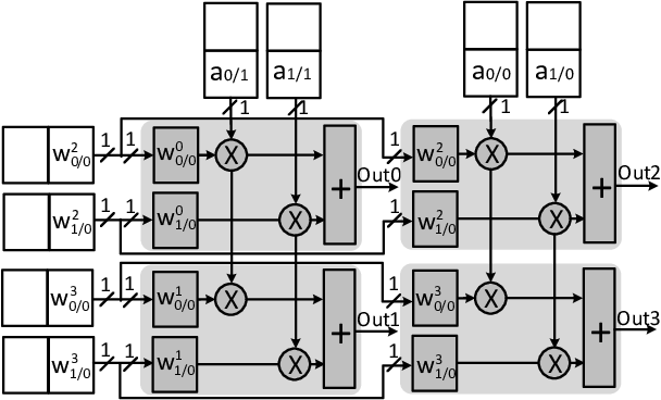
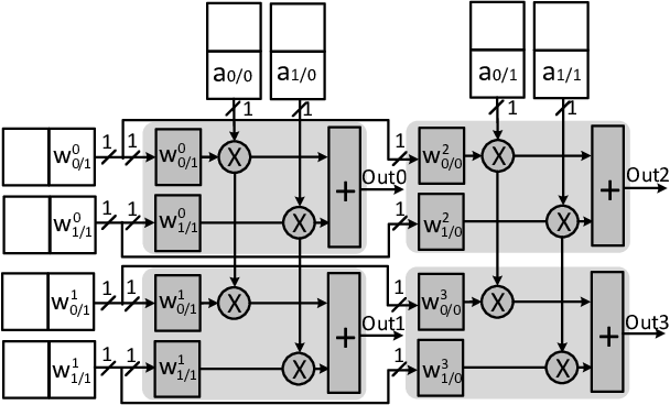
Figure 1b through Figure 1f show how LM would process an FCL. As Figure 1b shows, in cycle 1, the left column subunits receive the least significant bits (LSBs) and of activations and , and , , , and , the LSBs of four weights from filters 0 and 1. Each of these two subunits calculates two products (the product and accumulation would take place in the subsequent cycle adding one more pipeline stage, a detail the example omits for clarity) and stores their sum into its OR. In Figure 1c and cycle 2, the left column subunits now multiply the same weight bits with the most significant bits (MSBs) and of activations and respectively accumulate these into their ORs. In parallel, the two right column subunits load and , the LSBs of the input activations and , and multiply them by the LSBs of weights , , , and from filters 2 and 3. In cycle 3, the left column subunits now load and multiply the LSBs and with the MSBs , , , and of the four weights from filters 0 and 1. In parallel, the right subunits reuse their WR-held weights , , , and and multiply them by the most significant bits and of activations and (Figure 1d). In cycle 4 and Figure 1e, the left column subunits multiply their WR-held weights and and the MSBs of activations and and finish the calculation of output activations and . Concurrently, the right column subunits load , , , and , the MSBs of the weights from filters 2 and 3 and multiply them with and . In cycle 5 and Figure 1f, the right subunits complete the multiplication of their WR-held weights and and the MSBs of the two activations. By the end of this cycle, output activations and are ready as well.
In total it took 4+1 cycles to process 32 products (4, 8, 8, 8, 4 products in cycles 1 through 5, respectively). Notice that at the end of the 5th cycle, the left column subunits are idle, thus the WRs could have loaded another set of weights commencing the computation of a new set of outputs. In the steady state, with input activations and weights, this engine will be producing 8 terms every cycle thus matching the 2 throughput of the parallel engine. If the weights could be represented using only one bit, LM would be producing two output activations per cycle, twice the bandwidth of the bit-parallel engine.
In general, if the bit-parallel hardware was using bits to represent the weights while only bits were actually required, for the FCLs the LM engine would outperform the bit-parallel engine by . The LM would use an array of units, where the number of products DPNN processes per cycle. Each subunit would produce products. Since there is no weight reuse in FCLs, cycles are required to load a different set of weights to each of the columns. Thus having activations that use less than bits would not improve performance (but could improve energy efficiency).


Convolutional Layers: LM processes CVLs similarly to FCLs but exploits weight reuse across different windows to exploit a reduction in precision for both weights and activations. Specifically, in CVLs the subunits across the same row share the same weight bits which they load in parallel into their WRs in a single cycle. These weight bits are multiplied by the corresponding activation bits over cycles. Another set of weight bits needs to be loaded every cycles, where is the input activation precision. Here LM exploits weight reuse across multiple windows by having each subunit column process a different set of activations. Assuming that the bit-parallel engine uses bits to represent both input activations and weights, LM will outperform the bit-parallel engine by where and are the weight and activation precisions LM uses respectively.
3. Loom Architecture
This section describes the baseline fixed precision bit-parallel accelerator and the Loom architecture.
3.1. Data Supply and Baseline System
Our baseline design (DPNN) shown on Figure 2a is an appropriately configured data-parallel engine inspired by the DaDianNao accelerator (1) the de facto standard used for comparison in most accelerator studies. DPNN uses 16-bit fixed-point activations and weights. DPNN comprises inner product units (IP) each processing a different filter. Every cycle DPNN accepts as input activations and corresponding weights per filter out of filters. In the configuration shown and . The activations are broadcast to all IP units. Each IP unit multiplies each of the activations with one out of its weights, reduces the resulting 32b products with an adder tree, and accumulates the result into an output register. In total, every cycle, DPNN calculates products producing partial output activations.
An Activation Memory (AM) and a Weight Memory (WM) supply respectively the activations and the weights. An input activation buffer (ABin) buffers the input activations while an output activation buffer (ABout) temporarily buffers the output activations. For clarity, in our description we assume a single tile that processes up to 128 weights (8 filters) and 16 activations per cycle.
3.2. Loom
For LM to match our DPNN configuration it needs to process 128 filters concurrently and 16 weight bits per filter per cycle, for a total of weight bits per cycle. Alternatively, LM could process 32 filters over 64 windows, however, we leave this investigation for future work. LM also accepts 256 1-bit input activations each of which it multiplies with 128 1-bit weights thus matching the computation bandwidth of base in the worst case where both activations and weights need 16 bits. Figure 2b shows the Loom design. It comprises 2K Serial Inner-Product Units (SIPs) organized in a grid. Every cycle, each SIP multiplies 16 input activations with 16 weights and reduces these products into a partial output activation. The SIPs along the same row share a common weight bus, and the SIPs along the same column share a common activation bus. Accordingly, as in DPNN, the SIP array is fed by a weight bus and a activation input bus. Similar to DPNN, LM has an ABout and an ABin. LM processes both activations and weights bit-serially.
Reducing Memory Footprint and Bandwidth: Since both weights and activations are processed bit-serially, LM can store weights and activations in a bit-interleaved fashion and using only as many bits as necessary thus boosting the effective bandwidth and storage capacity of the weight memory and the AM. For example, given 2K weights to be processed in parallel, LM would pack first their bit 0 onto continuous rows, then their bit 1, and so on up to bit 12. DPNN would stored them using 16 bits instead. A transposer can rotate the output activations prior to writing them to AM from ABout. Since each output activation entails inner-products with tens to hundreds of inputs, the transposer demand will be low.
Convolutional Layers: Processing starts by reading in parallel 2K weight bits from memory, loading 16 bits to all WRs per SIP row. The loaded weights will be multiplied by 16 corresponding activation bits per SIP column bit-serially over cycles where is the activation precision for this layer . Then, the second bit of weights will be loaded into WRs and multiplied with another set of 16 activation bits per SIP row, and so on. In total, the bit-serial multiplication will take cycles. where the weight precision for this layer . Whereas DPNN would process 16 sets of 16 activations and 128 filters over 256 cycles, LM processes them concurrently but bit-serially over cycles. If and/or are less than 16, LM will outperform DPNN by . Otherwise, LM will match DPNN’s performance.
Fully-Connected Layers: Processing starts by loading the LSBs of a set of weights into the WR registers of the first SIP column and multiplying the loaded weights by the LSBs of the corresponding activations. In the second cycle, while the first column of SIPs is still busy with multiplying the LSBs of its WRs by the second bit of the activations, the LSBs of a new set of weights can be loaded into the WRs of the second SIP column. Each weight bit is reused for 16 cycles multiplying with bits 0 through bit 15 of the input activations. Thus, there is enough time for LM to keep any single column of SIPs busy while loading new sets of weights to the other 15 columns. For example, as shown in Figure 2b LM can load a single bit of 2K weights to SIP(0,0)..SIP(0,127) in cycle 0, then load a single-bit of the next 2K weights to SIP(1,0)..SIP(1,127) in cycle 1, and so on. After the first 15 cycles, all SIPs are fully utilized. It will take cycles for LM to process 16 sets of 16 activations and 128 filters while DPNN processes them in 256 cycles. Thus, when is less than 16, LM will outperform DPNN by and it will match DPNN’s performance otherwise.

| Convolutional Layers | ||||
| Network | 100% Accuracy | 99% Accuracy | ||
| Act. / Per Layer | W | Act. / Per Layer | W | |
| NiN | 8-8-8-9-7-8-8-9-9-8-8-8 | 11 | 8-8-7-9-7-8-8-9-9-8-7-8 | 10 |
| AlexNet | 9-8-5-5-7 | 11 | 9-7-4-5-7 | 11 |
| 10-8-10-9-8-10-9-8-9-10-7 | 11 | 10-8-9-8-8-9-10-8-9-10-8 | 10 | |
| VGGS | 7-8-9-7-9 | 12 | 7-8-9-7-9 | 11 |
| VGGM | 7-7-7-8-7 | 12 | 6-8-7-7-7 | 12 |
| VGG19 | 12-12-12-11-12-10-11-11-13-12-13-13-13-13-13-13 | 12 | 9-9-9-8-12-10-10-12-13-11-12-13-13-13-13-13 | 12 |
| Fully-Connected Layers | ||||
| 100% Accuracy | 99% Accuracy | |||
| Weights /Per Layer | Weights/Per Layer | |||
| NiN | N/A | N/A | ||
| AlexNet | 10-9-9 | 9-8-8 | ||
| 7 | 7 | |||
| VGGS | 10-9-9 | 9-9-8 | ||
| VGGM | 10-8-8 | 9-8-8 | ||
| VGG19 | 10-9-9 | 10-9-8 | ||
SIP: Bit-Serial Inner-Product Units: Figure 3 shows LM’s Bit-Serial Inner-Product Unit (SIP). Every clock cycle, each SIP multiplies 16 single-bit activations by 16 single-bit weights to produce a partial output activation. Internally, each SIP has 16 1-bit Weight Registers (WRs), 16 2-input AND gates to multiply the weights in the WRs with the incoming input activation bits, and a 16-input adder tree that sums these partial products. accumulates and shifts the output of the adder tree over cycles. Every cycles, shifts the output of and accumulates it into the OR. After cycles the Output Register (OR) contains the inner-product of an activation and weight set. In each SIP, a multiplexer after implements cascading. To support signed 2’s complement activations, a negation block is used to subtract the sum of the input activations corresponding to the most significant bit of weights (MSB) from the partial sum when the MSB is 1. Each SIP also includes a comparator (max) to support max pooling layers.
Dynamic Precision Reduction: So far we assumed that software provided profile-derived per layer activation and weight precisions (6). Lascorz et al., observed that the hardware can further shorten these precisions by inspecting the actual values at runtime (5). LM determines adjusts precision per group of 256 activations that it processes concurrently. Per bit position OR trees produce a 16-bit vector indicating the positions where any of the activations has a 1. A leading one detector identifies the most significant position and thus the precision in bits that is sufficient.
Processing Layers with Few Outputs: For LM to keep all the SIPs busy an output activation must be assigned to each SIP. This is possible as long as the layer has at least 2K outputs. However, in the networks studied some FCLs have only 1K output activations, To avoid underutilization, LM’s implements SIP cascading, in which SIPs along each row can form a daisy-chain, where the output of one can feed into an input of the next via a multiplexer. This way, the computation of an output activation can be sliced along the bit dimension over the SIPs in the same row. In this case, each SIP processes only a portion of the input activations resulting into several partial output activations along the SIPs on the same row. Over the next cycles, where is the number of bit slices used, the partial outputs can be reduced into the final output activation.
Other Layers: Similar to DaDN, LM processes the additional layers needed by the studied networks. To do so, LM incorporates units for MAX pooling as in DaDN. Moreover, to apply nonlinear activations, an activation functional unit is present at the output of the ABout. Given that each output activation typically takes several cycles to compute, it is not necessary to use more such functional units compared to DPNN.
Total computational bandwidth: In the worst case, with 16b activations and weights, a single product that would have taken DPNN one cycle to produce, now takes LM 256 cycles. Since DPNN calculates 128 products per cycle, LM needs to calculate the equivalent of products every 256 cycles. LM has SIPs each producing 16 products per cycle. Thus, over 256 cycles, LM produces products matching DPNN’s compute bandwidth.
Tuning the Performance, Area and Energy Trade-off: We can trade off some of the performance benefits to reduce the number of SIPs and the respective area overhead by processing multiple activation bits per cycle. The evaluation section considers 2-bit () and 4-bit () LM configurations which need 8 and 4 SIP columns and accommodate precisions that are multiple of 2 and 4, respectively. For example, for reducing the from 8 to 5 bits produces no performance benefit, whereas for the it would improve performance by .
4. Evaluation
This section evaluates Loom performance, energy and area and explores the trade-off between accuracy and performance comparing to DPNN and Stripes (7).
4.1. Methodology
Execution time is modeled via a custom cycle-accurate simulator and energy and area measurements are collected over layouts of all designs. The designs were synthesized for worst case, typical case, and best case corners with the Synopsys Design Compiler using a TSMC 65nm library. Layouts were produced with Cadence Innovus using the typical corner case synthesis results which were more pessimistic for LM than the worst case scenario. Power results are based on the actual data-driven activity factors. The clock frequency of all designs is set to 1GHz. The ABin and ABout SRAM buffers were modeled with CACTI (8) and AM and WM were modeled as eDRAM with Destiny (9). We first evaluate LM assuming that all the activations fit on chip and the weights can be read from off-chip memory without any bandwidth constraint to explore the design space without being affected by the choice of a particular off-chip memory. We conclude by investigating performance with a single-channel of low-power DDR4-4267.
4.2. Weight and Activation Precisions:
Table 1 reports the profile-derived per layer precisions of input activations and network precisions of weights for the CVLs and FCLs using the method of Judd et al. (6). Since LM’s performance for the CVLs depends on both and , we adjust them independently. We use per layer activation precisions and a common across all CVLs weight precision. We found little inter-layer variability for weight precisions but additional per layer exploration is warranted. Since LM’s performance for FCLs performance depends only on we only adjust weight precision for FCLs. The precisions that guarantee no top-1 accuracy loss for CVLs input activations vary from 5 to 13 bits and for weights vary from 10 to 12. When a 99% relative top-1 accuracy is still acceptable, the activation and weight precision can be as low as 4 and 10 bits, respectively. The per layer weight precisions for the FCLs vary from 7 to 10 bits.
| FULLY-CONNECTED LAYERS | CONVOLUTIONAL LAYERS | |||||||||||||||
| Network | Stripes | Loom 1-bit | Loom 2-bit | Loom 4-bit | Stripes | Loom 1-bit | Loom 2-bit | Loom 4-bit | ||||||||
| Perf | Eff | Perf | Eff | Perf | Eff | Perf | Eff | Perf | Eff | Perf | Eff | Perf | Eff | Perf | Eff | |
| 100% TOP-1 Accuracy | 100% TOP-1 Accuracy | |||||||||||||||
| NiN | n/a | n/a | n/a | n/a | n/a | n/a | n/a | n/a | 1.76 | 1.54 | 2.97 | 2.40 | 2.92 | 2.75 | 2.91 | 3.05 |
| AlexNet | 1.00 | 0.88 | 1.65 | 1.34 | 1.66 | 1.56 | 1.66 | 1.74 | 2.34 | 2.04 | 4.25 | 3.43 | 4.20 | 3.96 | 3.66 | 3.84 |
| 0.99 | 0.87 | 2.25 | 1.82 | 2.27 | 2.14 | 2.28 | 2.39 | 1.76 | 1.50 | 2.63 | 2.12 | 2.49 | 2.34 | 2.12 | 2.22 | |
| VGGS | 1.00 | 0.88 | 1.63 | 1.32 | 1.63 | 1.54 | 1.63 | 1.71 | 1.89 | 1.65 | 3.98 | 3.21 | 3.78 | 3.56 | 3.02 | 3.17 |
| VGGM | 1.00 | 0.88 | 1.63 | 1.32 | 1.64 | 1.54 | 1.64 | 1.72 | 2.12 | 1.86 | 4.12 | 3.33 | 3.69 | 3.47 | 3.34 | 3.50 |
| VGG19 | 1.00 | 0.88 | 1.62 | 1.31 | 1.63 | 1.53 | 1.63 | 1.71 | 1.34 | 1.17 | 2.17 | 1.76 | 2.09 | 1.97 | 2.03 | 2.13 |
| Geomean | 1.00 | 0.88 | 1.74 | 1.41 | 1.75 | 1.65 | 1.75 | 1.84 | 1.84 | 1.61 | 3.25 | 2.63 | 3.10 | 2.92 | 2.78 | 2.92 |
| 99% TOP-1 Accuracy | 99% TOP-1 Accuracy | |||||||||||||||
| NiN | n/a | n/a | n/a | n/a | n/a | n/a | n/a | n/a | 2.31 | 2.02 | 4.21 | 3.40 | 4.09 | 3.85 | 3.78 | 3.96 |
| AlexNet | 1.00 | 0.88 | 1.85 | 1.49 | 1.85 | 1.74 | 1.85 | 1.94 | 2.57 | 2.25 | 4.62 | 3.73 | 4.49 | 4.23 | 4.36 | 4.57 |
| 0.99 | 0.87 | 2.25 | 1.82 | 2.27 | 2.14 | 2.28 | 2.39 | 1.80 | 1.58 | 2.91 | 2.35 | 2.74 | 2.58 | 2.30 | 2.42 | |
| VGGS | 1.00 | 0.88 | 1.78 | 1.44 | 1.78 | 1.68 | 1.79 | 1.87 | 1.89 | 1.65 | 3.98 | 3.21 | 3.78 | 3.56 | 3.15 | 3.30 |
| VGGM | 1.00 | 0.88 | 1.79 | 1.45 | 1.80 | 1.69 | 1.80 | 1.89 | 2.12 | 1.86 | 4.49 | 3.63 | 4.03 | 3.79 | 3.64 | 3.82 |
| VGG19 | 1.00 | 0.88 | 1.63 | 1.32 | 1.63 | 1.54 | 1.63 | 1.71 | 1.45 | 1.27 | 2.28 | 1.84 | 2.21 | 2.08 | 2.07 | 2.17 |
| Geomean | 1.00 | 0.88 | 1.85 | 1.49 | 1.85 | 1.75 | 1.86 | 1.95 | 1.99 | 1.74 | 3.63 | 2.93 | 3.45 | 3.25 | 3.11 | 3.26 |


4.3. Performance and Energy Efficiency
Figures 4a and 4b show respectively the performance and energy efficiency of Loom, Stripes, and DStripes configurations relative to DPNN with the precision 100% profiles of Table 1 and for all layers combined. Stripes is based on Stripes which exploits only profile-derived per layer activation precisions and only for CVLs (7). DStripes incorporates dynamic prediction reduction (5).
On average, outperforms DPNN by more than while being more than energy efficient. When LM processes multiple bits per cycle the performance benefits are lower but energy efficiency improves up to . consistently outperforms Stripes and DStripes in performance and Stripes in energy efficiency. is more energy efficient than DStripes except for GoogleNet where its energy efficiency is within of DStripes.
Table 2 reports per network performance and energy efficiency for LM configurations relative to DPNN for the FCLs and CVLs separately, and for the 100% and 99% accuracy profiles. In general, outperforms and in most cases with the latter two being more energy efficient. On occasion the latter two outperform under the 100% accuracy profiles in FCLs. Since for LM the performance improvement in FCLs is only due to the use of lower weight precisions, processing multiple activation bits per cycle does not effect performance in the steady state. However, processing more activation bits per cycle reduces the initiation interval per layer an effect that becomes noticeable for small FCLs.
The table reports detailed results for Stripes. For FCLs, Stripes performance and energy efficiency suffer as it does not exploit weight precisions. With the 99% accuracy profiles, both performance and energy efficiency improve considerably for FCLs and CVLs. Performance with DStripes would be identical to Stripes for the FCLs. We do not present detailed results for DStripes due to space limitations noting that LM consistently outperforms DStripes while being more energy efficient except for the CVLs for GoogLeNet where the difference in energy efficiency is small.
| Network | Effective Precision Per Layer |
|---|---|
| NiN | 8.85-10.29-10.21-7.65-9.13-9.04-7.63- |
| 8.65-8.62-7.79-7.96-8.18 | |
| AlexNet | 8.36-7.62-7.62-7.44-7.55 |
| 6.19-5.75-6.80-6.28-5.34-6.70-6.31-5.02 | |
| -5.49-7.89-4.83 | |
| VGGS | 9.94-6.96-8.53-8.13-8.10 |
| VGGM | 9.87-7.55-8.52-8.16-8.14 |
| VGG19 | 10.98-9.81-9.31-9.09-8.58-8.04-7.89-7.86 |
| -7.51-7.20-7.36-7.47-7.61-7.66-7.66-7.63 |
4.4. Area Overhead
Post layout measurements were used to measure the area of DPNN and Loom. The configuration requires more area over DPNN while achieving on average a speedup. The and reduce the area overhead to and while still improving the execution time by and , respectively. Thus LM exhibits better performance vs. area scaling than DPNN.
4.5. Scaling
Thus far we assumed that all activations fit on chip and focused on a single LM configuration. We next consider configurations with practical on- and off-ship memory hierarchies. Specifically, we size the activation memory so that most layers can fit on-chip avoiding off-chip accesses that today require at least two orders of magnitude more energy a critical consideration in embedded systems. Accordingly, DPNN requires 2MB of activation memory (VGG19 requires 10MB which is impractical for embedded systems and thus has to spill activations off-chip). Since LM processes both activations and weights bit-serially, it naturally stores and communicates values on- and off-chip using the per layer precisions. As a result, LM requires only 1MB on-chip memory for the activations. However, since LM processes more filters concurrently compared to DPNN, it can benefit from a larger weight memory.
Figure 5 shows how average performance over all networks scales for different configurations where the number of SIPs is chosen to match the peak compute bandwidth (x-axis) of a bit-parallel accelerator. For example, the "128" configurations can perform the equivalent of 128 multiply-accumulate operations per cycle. For each configuration Figure 5 reports performance relative to DPNN and absolute performance as frames per second (fps). The figure reports results for the convolutional layers only and also for all layers. This is done because fully-connected layers are off-chip bound (and thus are affected by our choice of off-chip memory) whereas the convolutional layers are compute bound. Here we restrict attention to .
LM outperforms DPNN for all design points shown and can achieve real-time processing rates even for the "32" configuration. The relative performance advantage of LM drops for the larger configurations since LM requires more parallelism and suffers more from increased underutilization as the number of weight lanes grows. DStripes’s relative performance over DPNN remains constant for the range shown. LM outperforms DStripes up to the "128" configurations. At "256" LM and DStripes perform nearly identically and at "512" the latter performs better.
The figure also reports the weight memory capacity, the relative (vs. DPNN) area overhead, and the energy efficiency for the various LM configurations. For the "64" and "32" configurations LM requires and less memory in total than DPNN. However, for the "128" and the "256" configurations LM requires more memory than DPNN. Regardless, the performance benefits exceed the relative area overhead and thus LM provides a better performance/area trade-off than DPNN. For the "256" configuration energy efficiency suffers with LM. However, this measurement ignores the energy of off-chip traffic which is on average less with LM. Moreover, as CNNs evolve to process higher resolution images the size of activation memory increases significantly compared to the filter sizes which makes the effect of data compression more important (11). Thus we expect that for higher resolution images LM will ever more appealing.

| All LAYERS COMBINED | ||||||
|---|---|---|---|---|---|---|
| Network | Loom 1-bit | Loom 2-bit | Loom 4-bit | |||
| Perf | Eff | Perf | Eff | Perf | Eff | |
| 100% TOP-1 Accuracy | ||||||
| NiN | 3.38 | 2.73 | 3.32 | 3.13 | 3.31 | 3.48 |
| AlexNet | 5.66 | 4.57 | 5.61 | 4.57 | 4.95 | 5.19 |
| 3.19 | 2.57 | 3.02 | 2.84 | 2.80 | 2.93 | |
| VGGS | 5.72 | 4.62 | 5.46 | 5.13 | 4.42 | 4.63 |
| VGGM | 6.03 | 4.87 | 5.46 | 5.14 | 4.60 | 4.83 |
| VGG19 | 3.38 | 2.73 | 3.28 | 3.09 | 3.01 | 3.15 |
| Geomean | 4.38 | 3.54 | 4.20 | 3.95 | 3.76 | 3.94 |
4.6. Per Group Weight Precisions
Thus far we assumed that LM exploits software provided profile-derived per layer weight precisions (6). However, exploiting the approach of Lascorz et al. (10) LM can further trim the weight precisions at a finer granularity to boost the performance and energy efficiency of both FCLs and CVLs. The per group weight precisions can be detected at runtime similarly to the activation precisions, or can be detected statically and communicated via per group metadata.
Table 3 reports the average effective weight precision per layer for a group of 16 weights. The estimated performance and energy efficiency of Loom configurations relative to DPNN with the precision profiles of Table 3 and for all layers combined is shown in Table 4. For these estimates we assume that performance scales linearly with weight precision.
Exploiting the effective weight precisions yields a speedup of , , and over DPNN for , , and configurations, respectively. The energy efficiency of LM over DPNN is , , and for the aforementioned configurations.
5. Related Work
Due to space limitations, we limit attention to a few works that are the most related. We have already compared to Stripes (7) extended with dynamic prediction reduction (5).
Pragmatic’s performance for the CVLs depends only on the number of activation bits that are 1, but does not improve performance for FCLs (12). Further performance improvement may be possible by combining Pragmatic’s approach with LM’s but the costs per SIP may make this prohibitively expensive. Proteus exploits per layer precisions reducing memory footprint and bandwidth but requires crossbars per input weight (13). Loom does not need crossbars. Hardwired NN implementations naturally exploit per layer precisions (14). Loom does not require that the whole network fit on chip nor does it hardwire precisions. Furthermore, Loom further trims activations precisions at runtime.
6. Conclusion
This work presented Loom, a hardware inference accelerator for DNNs whose execution time for the convolutional and the fully-connected layers scales inversely proportionally with the precision used to represent the input data. LM can trade-off accuracy vs. performance and energy efficiency on the fly. Future work may consider extending LM to further exploit weight sparsity.
References
- (1) Y. Chen, T. Luo, S. Liu, S. Zhang, L. He, J. Wang, L. Li, T. Chen, Z. Xu, N. Sun, and O. Temam, “Dadiannao: A machine-learning supercomputer,” in Microarchitecture (MICRO), 2014 47th Annual IEEE/ACM International Symposium on, pp. 609–622, Dec 2014.
- (2) R. B. Girshick, J. Donahue, T. Darrell, and J. Malik, “Rich feature hierarchies for accurate object detection and semantic segmentation,” CoRR, vol. abs/1311.2524, 2013.
- (3) A. Y. Hannun, C. Case, J. Casper, B. C. Catanzaro, G. Diamos, E. Elsen, R. Prenger, S. Satheesh, S. Sengupta, A. Coates, and A. Y. Ng, “Deep speech: Scaling up end-to-end speech recognition,” CoRR, vol. abs/1412.5567, 2014.
- (4) R. Lukac, Computational photography: methods and applications. CRC Press, 2016.
- (5) A. D. Lascorz, S. Sharify, P. Judd, and A. Moshovos, “Dynamic stripes: Exploiting the dynamic precision requirements of activation values in neural networks,” CoRR, vol. abs/1706.00504, 2017.
- (6) P. Judd, J. Albericio, T. Hetherington, T. Aamodt, N. E. Jerger, R. Urtasun, and A. Moshovos, “Reduced-Precision Strategies for Bounded Memory in Deep Neural Nets ,” arXiv:1511.05236v4 [cs.LG] , 2015.
- (7) P. Judd, J. Albericio, T. Hetherington, T. Aamodt, and A. Moshovos, “Stripes: Bit-serial Deep Neural Network Computing ,” in Proc. of the 49th Annual IEEE/ACM Intl’ Symposium on Microarchitecture, 2016.
- (8) N. Muralimanohar and R. Balasubramonian, “Cacti 6.0: A tool to understand large caches,” 2015.
- (9) M. Poremba, S. Mittal, D. Li, J. Vetter, and Y. Xie, “Destiny: A tool for modeling emerging 3d nvm and edram caches,” in Design, Automation Test in Europe Conference Exhibition, March 2015.
- (10) A. Delmas, S. Sharify, P. Judd, M. Nikolic, and A. Moshovos, “Dpred: Making typical activation values matter in deep learning computing,” arXiv preprint arXiv:1804.06732, 2018.
- (11) W. Liu, D. Anguelov, D. Erhan, C. Szegedy, S. Reed, C.-Y. Fu, and A. C. Berg, “SSD: Single Shot MultiBox Detector,” arXiv:1512.02325 [cs.CV], 2016.
- (12) J. Albericio, A. Delmás, P. Judd, S. Sharify, G. O’Leary, R. Genov, and A. Moshovos, “Bit-pragmatic deep neural network computing,” in Proceedings of the 50th Annual IEEE/ACM International Symposium on Microarchitecture, MICRO-50 ’17, pp. 382–394, 2017.
- (13) P. Judd, J. Albericio, T. Hetherington, T. M. Aamodt, N. E. Jerger, and A. Moshovos, “Proteus: Exploiting numerical precision variability in deep neural networks,” in Proceedings of the 2016 International Conference on Supercomputing, p. 23.
- (14) T. Szabo, L. Antoni, G. Horvath, and B. Feher, “A full-parallel digital implementation for pre-trained NNs,” in IJCNN 2000, Proceedings of the IEEE-INNS-ENNS International Joint Conference on Neural Networks, 2000, vol. 2, pp. 49–54 vol.2, 2000.
- (15) S. Han, X. Liu, H. Mao, J. Pu, A. Pedram, M. A. Horowitz, and W. J. Dally, “Eie: Efficient inference engine on compressed deep neural network,” in Proceedings of the 43rd International Symposium on Computer Architecture, ISCA ’16, (Piscataway, NJ, USA), pp. 243–254, IEEE Press, 2016.
- (16) J. Albericio, P. Judd, T. Hetherington, T. Aamodt, N. Enright Jerger, and A. Moshovos, “Cnvlutin: Ineffectual-neuron-free deep neural network computing,” in 2016 IEEE/ACM International Conference on Computer Architecture (ISCA), 2016.
- (17) S. Zhang, Z. Du, L. Zhang, H. Lan, S. Liu, L. Li, Q. Guo, T. Chen, and Y. Chen, “Cambricon-x: An accelerator for sparse neural networks,” in 49th Annual IEEE/ACM International Symposium on Microarchitecture, MICRO 2016, Taipei, Taiwan, October 15-19, 2016, pp. 1–12, 2016.
- (18) A. Parashar, M. Rhu, A. Mukkara, A. Puglielli, R. Venkatesan, B. Khailany, J. Emer, S. W. Keckler, and W. J. Dally, “Scnn: An accelerator for compressed-sparse convolutional neural networks,” in Proceedings of the 44th Annual International Symposium on Computer Architecture, ISCA ’17, pp. 27–40, 2017.