Nongeneric positive partial transpose states
of rank five in dimensions
Leif Ove Hansen and Jan Myrheim
Department of Physics, Norwegian University of Science and Technology,
N-7491 Trondheim, Norway
August 24, 2026
Abstract
In dimensions, entangled mixed states that are positive under partial transposition (PPT states) must have rank at least four. These rank four states are completely understood. We say that they have rank since a state and its partial transpose both have rank four. The next problem is to understand the extremal PPT states of rank . We call two states -equivalent if they are related by a product transformation. A generic rank PPT state is extremal, and and both have six product vectors in their ranges, and no product vectors in their kernels. The three numbers are -invariants that help us classify the state. There is no analytical understanding of such states. We have studied numerically a few types of nongeneric rank five PPT states, in particular states with one or more product vectors in their kernels. We find an interesting new analytical construction of all rank four extremal PPT states, up to -equivalence, where they appear as boundary states on one single five dimensional face on the set of normalized PPT states. The interior of the face consists of rank states with four common product vectors in their kernels, it is a simplex of separable states surrounded by entangled PPT states. We say that a state is -symmetric if and are -equivalent, and is genuinely -symmetric if it is -equivalent to a state with . Genuine -symmetry implies a special form of -symmetry. We have produced numerically, by a special method, a random sample of rank -symmetric states. About fifty of these are of type , among those all are extremal and about half are genuinely -symmetric. All these genuinely -symmetric states can be transformed to have a circulant form. We find however that this is not a generic property of genuinely -symmetric states. The remaining -symmetric states found in the search have product vectors in their kernels, they inspired us to study such states without regard to -symmetry.
1 Introduction
Entanglement between subsystems of a composite quantum system is a phenomenon which has no counterpart in classical physics. Entangled quantum states show correlations in measurements which cannot be modelled within any local theory, including classical physics. A classical local description of such systems implies so called Bell inequalities [1], which are violated in experiments [2]. So entangled quantum states exhibit a nonlocality that excludes any local theory, though nonlocal deterministic theories are still possible.
Pure product states are the only pure quantum states that are not entangled, and they resemble pure classical states in that they have no correlations at all. By definition, a mixed quantum state is a statistical ensemble of pure quantum states, and it is represented mathematically by a density matrix. One single density matrix may represent many different ensembles. A basic postulate is that there is no way to distinguish experimentally between different ensembles represented by the same density matrix.
A mixed quantum state is said to be separable if it can be mixed entirely from pure product states. The entangled states are exactly those that are not separable. While the separability problem for pure states is solved entirely via Schmidt decomposition of state vectors, the problem of how to characterize the set of separable mixed states, and to decide whether a given mixed state is separable or entangled, is known to be a very difficult mathematical problem in general, and it has been demonstrated that operational procedures are NP-hard [3].
In recent years these problems have been given considerable attention, mainly due to the fact that quantum entanglement has found use in many applications. Many new developments require an understanding of entanglement as a resource, in areas such as quantum communication, quantum cryptography, and quantum computing. How to prepare, manipulate and detect entangled quantum states has become an important issue.
Sound operational methods or criteria for entanglement checking only exist for special cases and/or for low dimensional systems. The separable states have the property that they remain positive after partial transposition, they are PPT states. The set of PPT states is in general larger than the set of separable states, but the difference between the two sets is small in low dimensions, and in the and systems [4]. Thus the condition of positive partial transpose, known as the Peres separability criterion [5], is completely adequate as long as the system has dimension .
For systems of dimension , entangled PPT states, also known as states with bound entanglement, exist. It is these states that make up the difference between and , they are the states where the Peres separability criterion is not sufficient.
Another useful criterion is the range criterion, which states that if a state is separable then its range is spanned by a set of product vectors such that the range of the partial transpose is spanned by . It was shown that this criterion is independent from the PPT criterion, as there are PPT entangled states that violate the range criterion and there are NPT states satisfying it [6].
The close relation between PPT states and product vectors has been used to prove the separability of sufficiently low rank PPT states. It was shown that all PPT states of rank at most supported on a Hilbert space of dimension with , are separable [7].
For the system this means that the lowest possible rank of an entangled PPT state is four. Bennett et al. [8, 9] introduced a method for constructing low rank entangled PPT states by using unextendable product bases (UPBs). A UPB is defined as a maximal set of orthogonal product vectors which is not a complete basis of the Hilbert space. If one constructs an orthogonal projection onto the UPB, then its complementary projection is an entangled PPT state. The UPB construction is most successful in the case of rank four PPT states in the system, where it leads to a construction of all entangled PPT states of rank four [10, 11].
This UPB strategy fails for rank five states in the system, since a UPB must lie in the kernel of the state it defines, and no UPB has only four elements. The lack of such a simple construction method makes the characterization of entangled PPT states in the system a much more challenging problem for the rank five states than for the rank four states. We report here on a study of the rank five states, describing in particular several nongeneric forms.
A PPT state is partly characterized by two numbers , where is its rank and is the rank of its partial transpose. A necessary condition for a PPT state in dimension to be extremal is that [12]. Most of the states we have studied have rank , but it should be noted that states of rank and rank are also easy to find numerically, and they are generically extremal. There also exist PPT states of rank , but they can not be extremal [13].
Outline of the paper
The contents of the present paper are organized in the following manner.
In Sections 2 and 3 we review some linear algebra and introduce notation. We emphasize the importance of product vectors and product transformations in our study of low-rank PPT states in bipartite composite systems. It is useful to classify such a state by the number of product vectors in its range and kernel.
Since a generic subspace of dimension four contains no product vectors, a rank five state with product vectors in its kernel is nongeneric. In Section 4 we define a standard form for PPT states of rank five with four product vectors in the kernel. All these special PPT states of rank are nonextremal, but this scheme leads to a new method for constructing extremal PPT states of rank , and is highly relevant to our further study of nongeneric PPT states of rank , presented in Section 7.
In Section 5 we review some features regarding product vectors in generic subspaces of dimension five in the system. We also discuss nongeneric subspaces in the system, specifically how to construct pairs of orthogonal subspaces and with and , such that the number of product vectors in is nonzero.
In Section 6 a summary of our numerical results on rank five PPT states is presented. This includes data for the generic states with no product vectors in , and several nongeneric cases with up to four product vectors in . We also present some results from our random searches for -symmetric states.
In Section 7 we present a collection of nongeneric standard forms for orthogonal subspaces and , with dimensions five and four respectively. The nongeneric feature is that the number of product vectors in is nonzero. For the various and , we have produced PPT states of rank with and . The number of product vectors in is either six or infinite, while the number of product vectors in ranges from one to four. The latter is presented as a special case in Section 4.
Finally, in Section 8 we present a very special five-dimensional subspace of that contains only two product vectors, with one product vector in the orthogonal complement. We construct analytically a set of states found by transformation to a standard form of one particular rank nonextremal PPT state in this subspace. This nonextremal PPT state was found completely by chance in our random searches for -symmetric states.
2 Basic linear algebra
We want to review some basic concepts of linear algebra, partly in order to define our notation and make the paper self-contained, and partly in order to review some useful but less well known facts.
2.1 Density matrices
The natural structure of the set of Hermitian matrices is that of a real Hilbert space of dimension with the scalar product
| (1) |
The set of mixed states, or density matrices, is defined as
| (2) |
A density matrix has a spectral representation in terms of a complete set of orthonormal eigenvectors with eigenvalues ,
| (3) |
The spectral representation is one particular ensemble representation of . It implies that
| (4) |
The rank of is the number of eigenvalues . The matrices
| (5) |
are Hermitian and project orthogonally onto the two complementary orthogonal subspaces , the range of , and , the kernel (or null space) of .
When all we say that is positive (or positive semidefinite) and write . An equivalent condition is that for all . It follows from the last inequality and the spectral representation of that .
The fact that the positivity conditions are linear in implies that is a convex set, so that if is a proper convex combination of ,
| (6) |
then . Furthermore, since
| (7) |
when , it follows that
| (8) |
independent of , when is a proper convex combination as above. Since is independent of , so is = .
A compact (closed and bounded) convex set is determined by its extremal points, those points that are not convex combinations of other points in the set. The extremal points of are the pure states of the form with and . Thus the spectral representation is an expansion of as a convex combination of extremal points in where is the rank of .
2.2 Perturbations and extremality in
Let be a density matrix, and define the projections and as in Equation (5). Consider a perturbation of the form
| (9) |
where is Hermitian, and so that . The real parameter may be infinitesimal or finite.
We observe that if , or equivalently if , then there will be a finite range of values of , say with , such that and . This is so because the eigenvectors of with zero eigenvalue will remain eigenvectors of with zero eigenvalue, and all the positive eigenvalues of will change continuously with into eigenvalues of . Since is compact, we may choose and such that has at least one negative eigenvalue when either or . The negative eigenvalue becomes zero at or , this makes strictly larger than and strictly smaller than in both limits and .
The other way around, if for with , then is a convex combination of and for every in the open interval . Hence is independent of in this open interval, implying that and .
This gives us three equivalent formulations for the extremality condition of on . The state is extremal in if and only if
- –
There exists no with and .
- –
The equation for the Hermitian matrix has as its only solution (up to proportionality).
- –
There exists no with and .
We may replace the condition by the weaker condition . By standard perturbation theory it implies that the zero eigenvalues of do not change to first order in . Thus, the perturbation in Equation (9), with and infinitesimal, preserves the rank but not necessarily the range of .
2.3 Projection operators on
Using the projections and defined above we can define projection operators , , and on , the real Hilbert space of Hermitian matrices, as follows,
| (10) |
Here is the identity operator on . It is straightforward to verify that these are complementary projections, with , and so on. They are symmetric with respect to the natural scalar product on , hence they project orthogonally, and relative to an orthonormal basis for they are represented by symmetric matrices.
Relative to an orthonormal basis of with the first basis vectors in and the last basis vectors in , a Hermitian matrix takes the block form
| (11) |
with and . In this basis we have
| (12) |
and hence
| (13) |
3 Composite systems
In order to describe entanglement in quantum systems it is necessary to develop the basic theory of tensor product spaces. We do this for a bipartite system consisting of two subsystems A and B.
3.1 Product vectors
If then the tensor product spaces (a complex tensor product) and (a real tensor product) describe a composite quantum system with two subsystems A and B of Hilbert space dimensions and .
A vector then has components , where
| (14) |
A product vector has components . We see that is a product vector if and only if its components satisfy the quadratic equations
| (15) |
These equations are not all independent, the number of independent complex equations is
| (16) |
For example, if we get a complete set of independent equations by taking , , and .
Since the Equations (15) are homogeneous, any solution gives rise to a one parameter family of solutions where . A vector in a subspace of dimension has independent complex components. Since the most general nonzero solution must contain at least one free complex parameter, we conclude that a generic subspace of dimension will contain nonzero product vectors if and only if
| (17) |
The limiting dimension
| (18) |
is particularly interesting. In this special case a nonzero solution will contain exactly one free parameter, which has to be a complex normalization constant. Thus up to proportionality there will exist a finite set of product vectors in a generic subspace of this dimension, in fact the number of product vectors is [14]
| (19) |
A generic subspace of lower dimension will contain no nonzero product vector, whereas any subspace of higher dimension will contain a continuous infinity of different product vectors (different in the sense that they are not proportional).
These results hold for generic subspaces. It is trivially clear that nongeneric subspaces with low dimensions exist that contain product vectors. In the special case studied here, the limiting dimension given by Equation (18) is five, and the number of product vectors given by Equation (19) is six. As described in Section 8 we have found one special example of a five dimensional subspace with only two product vectors. Nongeneric cases are treated more generally in [11].
The facts that product vectors always exist in and higher dimensions, but not always in and lower dimensions, are special cases of a theorem proved by Parthasarathy for systems composed of any number of subsystems [15]. These results have profound implications for the construction of unextendible product bases.
3.2 Partial transposition and separability
The following relation between matrix elements
| (20) |
defines the partial transpose of the matrix with respect to the second subsystem B. The partial transpose with respect to the first subsystem A is where denotes total transposition. Since we work with Hermitian matrices, is the same as complex conjugation. The partial transposition is transposition of the individual submatrices of dimension in the matrix . If then .
A density matrix is called separable if it is a convex combination of tensor product pure states,
| (21) |
with , , and . It follows that
| (22) |
We denote the set of separable density matrices by .
The obvious fact that is positive when is separable is known as the Peres criterion, it is an easily testable necessary condition for separability. For this reason it is of interest to study the set of PPT or Positive Partial Transpose matrices, defined as
| (23) |
We may call it the Peres set. A well known result is that for , whereas is strictly larger than in higher dimensions [4].
We will classify low rank PPT states by the ranks of and respectively. Here we study the special case , then the ranks and are equivalent for the purpose of classification, because of the symmetric roles of the subsystems A and B, and the arbitrariness of choice of which subsystem to partial transpose.
3.3 Product vectors in the kernel and range
Recall that when , and similarly for . The identity
| (24) |
therefore implies, for a PPT state , that if and only if .
Let the number of product vectors in , and be respectively , , and . Then is also the number of product vectors in , and is characterized by . We find numerically that the generic entangled PPT states of rank are by this characterization states.
We write the product vectors in as
| (25) |
And likewise for ,
| (26) |
Since the two subspaces are orthogonal, it is necessary that for all , hence for every pair we must have either or .
3.4 The range criterion and edge states
If is the separable state given in Equation (21), then is spanned by the product vectors , and is spanned by the partially conjugated product vectors . No such relation is known to exist between product vectors in and when is an entangled PPT state.
The existence of a set of product vectors spanning the range of , such that the partially conjugated product vectors span the range of , is therefore seen to be a necessary condition for separability, called the range criterion [6]. Since there exist entangled states satisfying the range criterion, the condition is not sufficient.
Please note that the range criterion demands that there should exist at least one such set of product vectors, not that all product vectors in the ranges should be related by partial conjugation. For example, in dimensions, which is the case discussed here, when a separable state is a convex combination of five randomly chosen pure product states, and will contain exactly six product vectors each, but the sixth product vector in is not the partial conjugate of the sixth product vector in .
An edge state is defined as a PPT state that breaks the range criterion maximally, in the sense that there exists no product vector in the range of with its partial conjugate in the range of . All edge states are entangled by the range criterion.
It is straightforward to see that every extremal entangled PPT state must be an edge state. In fact, if and , then is not extremal, because is a PPT state for both positive and negative in some finite interval. The converse is not true: there exist plenty of edge states that are not extremal [13].
3.5 Extremality in
We will now describe the extremality test in , which follows directly from the extremality test in . We want to outline also how to use perturbations with various restrictions in order to calculate the dimensions of surfaces of states in of fixed ranks. Thus we are interested in perturbations that preserve the ranks of and simultaneously, but do not necessarily preserve the ranges.
As we did for , we define and as the orthogonal projections onto and . We then define
| (27) |
These are again projections on the real Hilbert space , and like and they are symmetric with respect to the natural scalar product on . We use these projection operators on to impose various restrictions on the perturbation matrix in Equation (9).
Testing for extremality in
Clearly is extremal in if and only if is the only simultaneous solution of the two equations and . Another way to formulate this condition is that there exists no , with both and
Since and are projections, the equations and together are equivalent to the single eigenvalue equation
| (28) |
Note that the operator is real symmetric and positive and therefore has a complete set of nonnegative real eigenvalues and eigenvectors.
When we diagonalize we will always find as an eigenvector with eigenvalue 2. If it is the only solution of Equation (28), this proves that is extremal in . If is a solution not proportional to , then we may impose the condition (replace by if necessary), and we know that there exists a finite range of both positive and negative values of such that , hence is not extremal in .
Perturbations preserving the PPT property and ranks
The rank and positivity of is preserved by the perturbation to first order in , both for and , if and only if . Similarly, the rank and positivity of is preserved if and only if . These two equations together are equivalent to the single eigenvalue equation
| (29) |
Again is real symmetric and has a complete set of real eigenvalues and eigenvectors. The number of linearly independent solutions for in Equation (29) is then the dimension of the surface through of rank PPT states.
We may want to perturb in such a way that , but not necessarily , that is, we only require and to have the same rank. Then the conditions on are that and , or equivalently
| (30) |
In this case the number of linearly independent solutions for is the dimension of the surface through of rank PPT states with fixed range .
3.6 Product transformations
A product transformation of the form
| (31) |
where is a normalization factor and , , preserves positivity, rank, separability and other interesting properties that the density matrix may have. It preserves positivity of the partial transpose because
| (32) |
A transformation of the form of Equation (31) is also sometimes referred to as a local SL-transformation.
The range and kernel of and transform in the following ways,
| (33) |
We say that two density matrices and related in this way are -equivalent. The concept of -equivalence is important because it simplifies very much the classification of the low rank PPT states. Since this -equivalence is transitive it generates equivalence classes of matrices.
-symmetry under partial transposition
We say that the state is -symmetric if and are -equivalent, that is, if
| (34) |
Since SL-transformations of product type preserve the number of product vectors in a subspace, any transformation must transform the set of product vectors in the range of to the set of product vectors in the range of , so for -symmetric states we must have . If the product vectors in are with and the product vectors in are for , then
| (35) |
Since our understanding of the relation between the sets and is quite limited for entangled states, it is difficult to say much in general about what makes some states -symmetric and others not.
Genuine -symmetry
We say that a state is genuinely -symmetric if there exists a transformation
| (36) |
such that . The transformation of implies that
| (37) |
when we define . The genuine -symmetry implies further that
| (38) |
and hence
| (39) |
and with . This shows that genuine -symmetry implies -symmetry, and Equation (39) requires that preserves the trace of ,
| (40) |
A sufficient but not necessary condition for this trace preservation is that is unitary.
The relation implies that has some special properties. One implication is that , and hence . If we multiply by some phase factor , then is multiplied by , and in this way we may redefine such that .
We conclude that for the state to be genuinely -symmetric it must be -symmetric with a transformation of the form given in Equation (39). For the system, would have the form
| (41) |
with and .
Since the transformation has the form in the case of genuine -symmetry, by Equation (35) the product vectors in and will be related by the transformations and . This is a necessary condition for genuine -symmetry which may be tested as soon as we know the product vectors in and .
Assume that for a given PPT state we find that and are related by a transformation of the form given in Equation (39). Then a further problem to be solved is to find a transformation that demonstrates explicitly the genuine -symmetry of . Here is completely arbitrary, hence the simplest solution is to take . Next we have to solve the equation for . We find one particular solution by assuming that . This gives the equation , and the solution is the matrix square root,
| (42) |
Since , this is consistent with the assumption .
It should be noted that the matrix square root is in general many valued. A standard solution is found by the rapidly converging Newton–Raphson method: starting with we iterate the substitution
| (43) |
We find in practice that this solution for always works.
4 The rank extremal PPT states revisited
The rank extremal PPT states in dimension are well understood [10, 11, 16, 17]. They are all -equivalent to states constructed from unextendible product bases (UPBs), and they all have exactly six product vectors in their kernels. A construction method not using UPBs was discussed in [17], and as part of that discussion the structure of a PPT state with at least four product vectors in was derived.
In the present section we will review and expand on the discussion given in [17]. This is relevant for our present study of nongeneric rank PPT states, and it leads to a new construction of the rank extremal PPT states.
Given a PPT state of rank at most five, and four product vectors in , in some definite but arbitrary order. We assume that any three vectors and any three vectors are linearly independent. Then we may perform a product transformation as in Equation (31), and subsequent normalizations, so that the vectors take the form
| (44) |
and
| (45) |
The transformation is unique. In this four dimensional subspace there exist no other product vectors. The real form of the product vectors implies that .
It is equally easy to see that there exist exactly six product vectors in the orthogonal subspace. In fact, in order to have for all and , we must have for each pair that either or . Since any three vectors and any three vectors are linearly independent, a vector can be orthogonal to at most two vectors, and a vector can be orthogonal to at most two vectors. This gives the six possibilities for orthogonality listed in the table.
The unique solution is the following:
| (46) |
| (47) |
The five dimensional subspace given by (47) defines a face of dimension . Recall that
| (48) |
In terms of the face , Equation (48) means that and , or equivalently, that . Equation (48) restricts to have the following form, with real coefficients ,
| (49) |
This form implies that . Since is a face on , we see that is a face on , and the intersection is a face on . Equation (49) with the normalization condition
| (50) |
shows that the face has dimension five.
The state defined in Equation (49) is a linear combination, but not necessarily a convex combination, of the six pure product states,
| (51) |
Since the matrices are linearly independent, and there are no other pure product states in , we see that is separable if and only if all the coefficients are nonnegative. However, we will now see that it is possible for to be an entangled PPT state even if one of the coefficients is negative.
An eigenvalue of , and of , is a root of the characteristic polynomial
| (52) |
with
| (53) |
If we start with for , then is a rank separable state. If we next change the coefficients continuously, will continue to have five positive eigenvalues until we get . Hence the equation defines the boundary of the set of density matrices, and also of the set of PPT states since .
We know that the boundary is not reached before at least one coefficient becomes zero or negative. If two coefficients become zero simultaneously, then and we have reached a boundary state which is separable. To get negative coefficients while is a rank PPT state we have to make one coefficient negative before the others. Let us say, for example, that , and that we want to make also negative, while for . Then we first have to make , in which case and we have already crossed the boundary .
In conclusion, the entangled boundary states have for , and they have one negative and five positive coefficients satisfying the equation
| (54) |
Thus the boundary consists of two types of states.
- 1.
Separable states that are convex combinations of up to four of the pure product states .
- 2.
Rank entangled PPT states that are linear combinations of all the six pure product states with exactly one negative coefficient.
It is well known that rank entangled PPT states are extremal.

Figure 1 shows an example of a two dimensional section through the five dimensional face of defined by Equations (51) and (50). The section through is the hexagon with corners to . In Table 2 we have listed the coefficients , multiplied by 12, that define the states to by Equation (51). The hexagon is reflection symmetric about two axes.
| 0 | 0 | 3 | 6 | 6 | 3 | |
| 1 | 0 | 0 | 1 | 2 | 2 | |
| 6 | 3 | 0 | 0 | 3 | 6 | |
| 2 | 2 | 1 | 0 | 0 | 1 | |
| 3 | 6 | 6 | 3 | 0 | 0 | |
| 0 | 1 | 2 | 2 | 1 | 0 |
The most general rank entangled PPT states
Consider a general rank entangled PPT state in dimensions. It is known that any such state is extremal, and has exactly six product vectors in its kernel. We can now see that it is -equivalent, in no less than 360 different ways, to such states on the boundary of the five dimensional face of that we have described here. The 360 transformations are found in the following way.
Pick any four of the six product vectors in , this can be done in 15 different ways. Order them next in one of the 24 possible ways. Altogether there are possibilities. There is then a unique product transformation that transforms the four product vectors to the form given in Equation (45). We know that it must transform the state into one of the rank states described by the Equations (51), (50), and (54), since these are the only rank entangled PPT states of this form.
5 Rank PPT states in dimensions
Our main purpose with the present study has been to try to understand the rank entangled PPT states in dimensions. In particular, we would like to understand better the relation between and when is a rank PPT state. A natural question is whether is -symmetric, as defined in Equation (34), so that with .
The product vectors in and are very useful for answering the question of -symmetry, especially when both these spaces have dimension five. By Equation (16), the number of constraints to be satisfied by a product vector is , thus is precisely the critical dimension at which every subspace contains one or more product vectors, and a generic subspace contains a finite number of product vectors, exactly six in this case. From these product vectors one may construct invariants that may be used to test whether the two spaces are related by some product transformation , which is a necessary condition for the -symmetry of the state .
5.1 Generic five dimensional subspaces
Any set of five product vectors in a generic five dimensional subspace may be transformed by an -transformation, followed by suitable normalizations, to the standard form [17]
| (55) |
with as real or complex parameters. By generic we here mean that any three vectors in and in are linearly independent. There will also be a sixth product vector which is a linear combination of the above five. The parameters are determined by the following ratios of determinants,
| (56) |
| (57) |
All the parameters are invariant under -transformations. Hence for given vectors and not on standard form these formulas may be used to calculate the values of the parameters without actually performing the transformation to standard form.
Though only and occur in Equations (56) and (57), since the numbering is arbitrary all six product vectors must be taken into consideration when calculating the invariants. Different permutations of the six product vectors will in general give different values for the invariants.
The standard form in Equation (55), or equivalently the invariants defined in Equations (56) and (57), can be used to check whether and are -equivalent. We must find the six product vectors in and , in some order. Then we either transform these to the standard form in Equation (55), or calculate directly the invariants for both subspaces. For the comparison we should try all the permutations of the six product vectors in one of the two subspaces. If the invariants so calculated are identical for a given permutation, then and can be transformed by a unique -transformation to the standard form in Equation (55) with the same values of . The transformations of both spaces to a common standard form then define a unique transformation from to . It is then easy to check whether for some .
Note that different permutations may give identical sets of invariants, but different that transform between the two spaces. We may have to try all of these transformations in order to find one that transforms into .
Note also that the partial transpose of with respect to subsystem is . If is -symmetric under this partial transposition, then it means that the invariants of will be the complex conjugates of the invariants of . In general, this type of symmetry is just as likely to occur.
Separable rank states
In a generic five dimensional subspace of containing six normalized product vectors , we may construct a five dimensional set of separable states as convex combinations
| (58) |
with and . Hence all the separable states in the subspace are contained in a simplex with the six pure product states as vertices. The partial transpose of is
| (59) |
where is the partial conjugate of . The six partially conjugated product vectors will be linearly independent in the generic case, hence the separable states in the interior of the simplex will have rank .
On the boundary where one coefficient vanishes, will be a rank PPT state. In this case five of the product vectors in and in are partial conjugates of each other, whereas the sixth product vectors in the two spaces are related in a more complicated way, unless all the vectors are real.
The surface of generic rank PPT states
It is known that a generic four dimensional subspace is not the range of any entangled rank PPT state [10]. It appears however in our numerical investigations that every generic five dimensional subspace is the common range of extremal and hence entangled rank PPT states that together form an eight dimensional surface [17]. It is an interesting numerical observation that the dimension of the surface of rank PPT states in a generic five dimensional subspace is higher than the dimension of the simplex of separable states.
In order to compute this surface numerically we consider the perturbation
| (60) |
with and satisfying Equation (30).
We find eight linearly independent solutions for in addition to the trivial solution , meaning that the surface has dimension eight.
5.2 Nongeneric five dimensional subspaces
By definition, for a generic set of vectors in any subset of three vectors will be linearly independent. For a generic rank PPT state , the range contains six product vectors . A nonzero vector can at most be orthogonal to two vectors , and a nonzero can at most be orthogonal to two , hence can at most be orthogonal to four . Since it is clear that in the generic case it is not possible to have a product vector in , as described in Section 3.3. Thus generic states must have .
In order to construct pairs of orthogonal subspaces and with and , such that contains one or more product vectors, we must alter the generic linear dependencies of the and vectors. Instead of the generic condition that any three vectors , and any three , must be linearly independent and span , we introduce the condition that any four vectors must span . Then it is possible to have one or more product vectors with each orthogonal to and orthogonal to where is some permutation of .
In the above sense it is the subspaces that are interesting, and to a lesser degree the states themselves. A general characterization of two orthogonal subspaces and with regard to the number of product vectors they contain, is then .
Since if and only if , it is clear that the kernels of and are related when they contain product vectors. In particular, if is real then . As long as , which is always the case in the examples we have constructed here, we can always choose a standard form where all the vectors and are real.
6 A summary of numerical results
We summarize here the main results of our numerical investigations. For ease of reference we number the cases from I to VII.
6.1 Generic states: Case I
The generic rank PPT state is an extremal and hence entangled state. By definition, a generic state is found in a completely random search for rank PPT states. The number of generic rank PPT entangled states we have generated are in the thousands. None of them are -symmetric, and since they are extremal they are also edge states. The partial transpose of a generic rank PPT state is again a generic rank PPT state.
Unfortunately, we have made little progress in understanding these states. We have no general understanding of the relation between the five dimensional subspaces and , which both contain six product vectors. Thus we have found no basis for a more detailed classification, in terms of canonical forms allowing us to use analytical methods in their construction.
6.2 -symmetric states: Case Ia
The complete set of PPT states of rank has dimension 48, and the set of -transformations has dimension , so the set of equivalence classes of rank states with respect to -transformations will have dimension 16, see [17]. Hence in a completely random search for PPT states of rank we will never find two states belonging to the same equivalence class. We also find that such a state , which we call generic, does never belong to the same -equivalence class as its partial transpose .
This shows that -symmetric states can be found numerically only by conducting restricted searches. We will describe now two different search methods. For some reason that we can only guess, the second method produces states of a more special kind than the first method.
Method I
An easy general procedure for constructing numerically PPT states of specified rank that are genuinely -symmetric, is to construct positive matrices that are symmetric under partial transposition, and then subject them to random -transformations.
Method II
Method I leaves open the question whether there exist PPT states that are -symmetric but not genuinely -symmetric. In order to answer this question, we produced in a random search more than a hundred -symmetric PPT states of rank , together with their associated -transformations. We find that 50 of these are states like the generic rank states, and we will now describe these. Our search was rather special in the sense that we looked for transformations of the form (34) with , i.e. transformations that are trace preserving. This choice allowed for the possibility that the states found might be genuinely -symmetric.
Out of the 50 states, about half are in fact genuinely -symmetric, as defined by Equation (36). To test for genuine -symmetry of a state we compare the transformation from to , found during the search, to the special form given in Equation (41). If it is of the wanted form, we construct the transformation from (42). If it is not of the wanted form, we have to produce more transformations, until we either find one of the wanted form, or decide that probably none exists.
We consider two transformation matrices to be identical if they differ only by a phase factor. For the -symmetric states that are not genuinely -symmetric, we find only one transformation from to . By definition, this is never of the form given in Equation (41). For the states of genuine -symmetry found by method II, the number of transformations we find is always three, and out of these there is only one that has the form given in Equation (41).
A special class of states proposed by Chruściński and Kossakowski have what they call the circulant form [18]
| (61) |
As long as the matrices , , and are positive, then so is , since the eigenvalues of are the eigenvalues of the submatrices , , and . There are similar additional constraints on the elements and in order for to be a PPT state.
Interestingly, all the genuinely -symmetric PPT states of rank which we have produced by method II, can be transformed by product transformations to the form (61). This property is all the more surprising, since none of the states produced by method I have the same property. We will now describe how to find the transformations.
As already mentioned, for such a state we always find three different product transformations , , and such that
| (62) |
Exactly one of them is of the form (41). There are six transformations, not necessarily different, of the form
| (63) |
transforming from back to . It does not matter which of the six transformations we choose. We find that with suitable normalization the equation is satisfied, and we have the eigenvalue decompositions
| (64) |
where the two sets of three eigenvalues and are both in arbitrary order, with . The eigenvectors are orthonormal, like the eigenvectors . The transformation with
| (65) |
is such that either or , depending on the permutation of the eigenvectors of and .
The fact that the genuinely -symmetric PPT states of rank produced by method II are of a more special type than those produced by method I, in that they can be transformed to the circulant form (61), needs an explanation. We guess that it is due to the existence of three product transformations from to , rather than one. Presumably it is easier to find a transformation when three solutions exist. Hence, we introduce a bias when we search simultaneously for a state of rank five and a transformation such that .
6.3 Nongeneric states: Cases II to VII
Our searches for -symmetric states have also produced a small number of states that have the nongeneric property, in addition to being -symmetric, that they have product vectors in their kernels. In particular, the very special subspace of type discussed in Section 8 is identified from four -symmetric states of type found in these random searches.
In Section 7, we discuss standard forms of states that are generically not -symmetric, but have the properties that and . We have generated numerically and studied nongeneric states having from one to four product vectors in the kernel, as discussed in Section 5.2. We define standard forms for nongeneric orthogonal subspaces and of dimensions five and four, respectively, with various numbers of product vectors. We take the product vectors in to have the standard form given in Equation (45), using only the first vectors. We have then produced a large number of PPT states of rank with and . We have studied the following nongeneric cases.
Case II, . Then contains from Equation (45), and is defined by Equation (83). The rank PPT states found are all extremal and of type .
Case III, . This is the special subspace presented in Section 8, producing both extremal and nonextremal entangled rank PPT states. The extremal states are of type . Some of the nonextremal states are of type , others are symmetric under partial transposition and therefore of type .
Case IV, . Then in the standard form contains , and is defined by Equation (75). The rank PPT states found are all extremal and of type .
Case V, , where contains , and is defined by Equation (67). The rank PPT states found are all nonextremal and of type .
Case VI, . This is the case discussed in Section 4, with defined by Equation (46). It gives a new way of constructing the extremal rank PPT states.
Case VII, . contains from Equation (45), whereas is defined by Equation (78) and contains an infinite number of product vectors. The resulting states include both extremal and nonextremal states, and also some interesting rank PPT states. We know that the latter do not exist in generic subspaces [17].
Table
Using the projection operators and extremality tests outlined earlier, we can calculate the dimensions of the surfaces defined by Equations (28)–(30) for the various types of states. We use the abbreviation for the operation that preserves the range of both and , for the preservation of the rank of both and , and finally and for the two other projections. The dimension given by has been subtracted Note that for many of the states the dimension defined by is zero, proving that the state is extremal and therefore entangled.
Presented in Table 3 are data for the various random rank PPT states we have produced. They were produced in large numbers with the exception of the extremal states, where a total of 15 states were produced. As we would expect, none of the states found were -symmetric, except in case Ia where the search was restricted to -symmetric states.
In addition to the dimensions defined above, we also indicate whether the states are edge states and whether they satisfy the range criterion, as defined in Section 3.4.
| Case | Edge | Range | |||||
| I, Ia | 48 | 8 | 8 | 0 | Yes | No | |
| II | 49 | 9 | 9 | 0 | Yes | No | |
| III | 49 | 9 | 9 | 0 | Yes | No | |
| IV | 50 | 10 | 10 | 0 | Yes | No | |
| V | 51 | 11 | 11 | 3 | No | No | |
| VI | 52 | 12 | 12 | 5 | No | Yes | |
| VII | 50 | 12 | 12 | 0 | Yes | No | |
| 50 | 11 | 11 | 6 | No | No | ||
| VIIa | 50 | 15 | 15 | 9 | No | No |
7 Nongeneric rank PPT states
We present here several standard forms for nongeneric orthogonal subspaces and of dimensions five and four. The set of parameters is usually assumed to be chosen in a generic, or completely random manner. One may however also investigate certain nongeneric choices for these coefficients.
These standard forms can be used to construct nongeneric rank PPT states with a range defined by the given standard form, and with . Some of these constructions give states that generically are extremal in and therefore entangled, while some return generically only nonextremal states.
Case V:
Given three product vectors in the kernel of we can make a product transformation so that we get for these for from Equation (45). We choose the orthogonality relations
| (66) |
A standard form for the six product vectors in the range of is then
| (67) |
| (68) |
Let be the matrix that results from removing the rows of zeros, i.e. the rows one, five, and nine from , then
| (69) |
Since we want the six product vectors to span a five dimensional space we require that . This equation determines the sixth parameter uniquely if we choose random values for five of the parameters .
We impose the further restrictions that all the six parameters should be nonzero, and that
| (70) |
Then the three vectors are linearly dependent, and so are and , but these are the only sets of three vectors that are linearly dependent. In the same way, the only sets of three linearly dependent vectors are , then , and . These linear dependencies make it possible for the three product vectors , and only these, to be orthogonal to all the six product vectors . One may check that with these choices of parameters there are no more product vectors that are linear combinations of the six vectors .
It should be noted that with our standard form for the three product vectors we still have a further freedom of doing diagonal product transformations. In this way we may actually reduce the number of parameters in our standard form from six to one, setting for example . We must then set in order to satisfy all the conditions. Setting we then get
| (71) |
A PPT state with spanned by the product vectors and with must also have , since are real. For given and these restrictions on reduce our search for such states to a seven dimensional subspace of . Six of the seven dimensions are spanned by the pure product states , with normalization factors , and there is only one dimension left where there is room for entangled PPT states. With and defined as in Equation (71) the seventh direction is given by the matrix
| (72) |
In random numerical searches we have produced different sets of six product vectors and hundreds of rank PPT states in the corresponding seven dimensional subspace of . All the states we find are entangled but not extremal. The only extremal PPT states in this subspace are the six pure product states and a four dimensional surface of rank states. The states define a five dimensional simplex of separable states, which contains two special equilateral triangles with corners and .
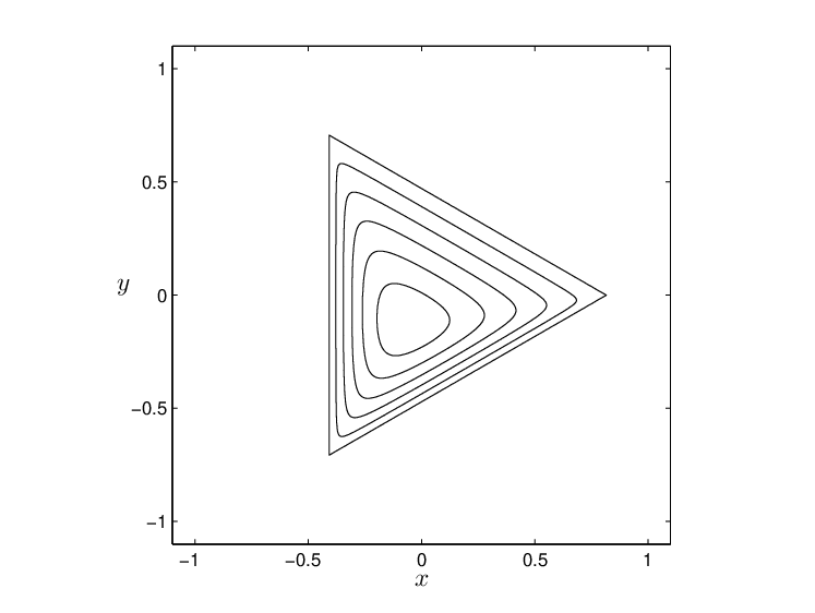
A convex combination of an arbitrary rank extremal PPT state and an arbitrary separable state from one of the two special triangles is always a rank entangled PPT state, and every rank PPT state of the above form can be constructed in this way. Thus, it lies inside a three dimensional set of rank PPT states bounded by an equilateral triangle, either or , and a two dimensional surface of extremal rank PPT states. An example of this geometry is shown in Figure 2. It implies that when is a rank PPT entangled state there are always three product vectors such that . The two possible sets of three are or . Since there are less than five such product vectors, the range criterion is not fulfilled.
A separable state mixed from product states has rank if . It has rank and lies in the interior of the simplex if . Rank entangled states arise in many ways, for example as convex combinations of one rank extremal state and pure product states from both special triangles, for example and . Ranks higher than six are of course impossible, since contains the three product vectors . Another consequence of the last fact is that contains six product vectors of the form in Equation (68), usually with other values for the coefficients .
We conclude that all of the rank states produced in these searches are entangled nonextremal states that are neither edge states nor satisfy the range criterion.
Case IV:
Given two product vectors in the kernel of we can always make a product transformation so that we get for these for from Equation (45).
We have the freedom of doing further product transformations with
| (73) |
In order to have six product vectors orthogonal to , one possibility is to impose the following orthogonality conditions,
| (74) |
These conditions are satisfied when the six product vectors in the range of have the standard form
| (75) |
with . We then get
| (76) |
We may generate random values of the coefficients defining any five of the six product vectors . Then we always find a sixth product vector, unique up to normalization, which is a linear combination of the five. The complete set of six product vectors then has rank five and automatically takes the form given in Equation (76). It is straightforward to check that are the only product vectors orthogonal to all the .
We generate rank PPT states with . With the additional restriction that the two fixed product vectors and should be in , the search can be restricted to an 11 dimensional subspace of the 81 dimensional space of Hermitian matrices.
With different sets of product vectors generated in this way we have produced numerically, by random searches, hundreds of rank PPT states. They are all extremal. Hence they are also edge states, that is, when we never have . The partial transpose of such a state always has the same characteristics, i.e. there are six product vectors in of the form given in Equation (76), but with different values of the coefficients .
In summary, all the states produced in this way are extremal states.
Case VII: with symmetric orthogonality relations
Observe that for the above standard form given in Equation (75), the orthogonality relations in Equation (74) overlap. This has been done intentionally, and the reason will become clear when we now try to impose the more symmetric orthogonality relations
| (77) |
This would give six product vectors in on a standard form
| (78) |
where . As compared to Equation (83) it means that we set . We then get
| (79) |
Omitting one of the six product vectors gives . However, omitting for example , we can find no sixth product vector of the form in the five dimensional subspace. On the other hand, there will be infinitely many product vectors that are linear combinations of . In fact, and must be linear combinations
| (80) |
and then for any the product vector with
| (81) |
will be a linear combination of . All these product vectors lie in a three dimensional subspace of a subspace.
Our search for rank PPT states with and can now be restricted to a 13 dimensional subspace of . Using five such randomly generated product vectors to create subspaces of dimension five, we have produced numerically by random searches hundreds of rank PPT states. Most of the states we find are separable, but we also find a very small number of extremal rank PPT states.
We find that 11 of the 13 dimensions in represent unnormalized separable states, and the entangled PPT states account for the last two of the 13 dimensions. This can be understood as follows. The product vectors span a three dimensional subspace containing infinitely many product vectors. These product vectors generate a set of unnormalized separable states of dimension nine, the same as the complete set of unnormalized density matrices on the three dimensional subspace. In addition we get two more dimensions of separable states from the product vectors and .
Note that a separable state mixed from more than three product vectors in the subspace will have rank . Hence, if we mix in also one or both of we will get separable states of rank or rank , respectively.
The partial transposes of the states we construct numerically have the same characteristics, thus all the states are of type . It is noteworthy that it is possible for an extremal rank PPT state to have infinitely many product vectors in its range.
Case II:
Given a product vector in the kernel of we may perform a product transformation as in Equation (31) so that the vector after normalization take the form from Equation (45).
This transformation is not unique, and we have the freedom of doing further transformations with
| (82) |
We assume that the six product vectors in the range of have the standard form
| (83) |
where . They are then orthogonal to because
| (84) |
The normalization in Equation (83) presupposes that the third component of every vector is nonzero. There is no loss of generality in this assumption, because of the freedom we have to do product transformations. This freedom could actually be used to reduce the number of parameters in the standard form given in Equation (83).
In our numerical searches we generate, for example, random values for the coefficients for . This is then a generic case in which span a five dimensional subspace, and there will be a unique solution for such that lies in this subspace. There are no other product vectors in the subspace, in the generic case.
Furthermore, there can be no product vector orthogonal to all , apart from . In fact, can at most be orthogonal to three vectors , because any four of the vectors span . Similarly, can at most be orthogonal to three vectors . The only set of three linearly dependent vectors is , and the only set of three linearly dependent vectors is . The only possibility is therefore that with and with , implying that .
We generate rank PPT states with this subspace as range. In general, there is a 25 dimensional real vector space of Hermitian matrices operating on a fixed subspace of dimension five. However, when we are searching for a PPT state with , we have the additional restriction that the partially conjugated product vector must be in . This reduces the 25 dimensions to 17, because the equation gives the four extra complex equations with and . It is straightforward to find numerically rank PPT states in this 17 dimensional space of Hermitian matrices.
In random searches we have produced hundreds of such states for many different sets of product vectors . All states produced in this manner are extremal. Hence they are edge states, that is, when we never have . We find that the partial transpose always has the same characteristics as , i.e. there are six product vectors in of the form in Equation (83), but with different values for the coefficients .
So in our classification all these states are extremal states.
8 Case III: An exceptional subspace of type
A generic five dimensional subspace of contains exactly six product vectors. Obviously, a nongeneric five dimensional subspace may well contain infinitely many product vectors, if it contains a whole product space , , or . On the other hand, it may also contain less than six product vectors, if the set of equations in (15) have degenerate solutions [11]. The maximum dimension of an entangled subspace, i.e. a subspace that does not contain any product vectors, is known from [15], and for the system the limiting dimension is four. So any subspace of of dimension five or higher must contain at least one product vector. We describe here a very special subspace of .
In our random searches for rank PPT states with the special symmetry property that the state and its partial transpose are -equivalent, we have found four such states with . A further special property of these states is that , i.e. there is exactly one product vector in . The states are not extremal, since three of them lie on a line between a pure product state and a rank extremal PPT state, whereas one lies inside a two dimensional region bounded by a closed curve of rank extremal PPT states.
Further numerical random searches for rank PPT states with the same ranges as the nonextremal rank PPT states described above, but not restricted to -symmetric states, reveal extremal rank PPT states of type . It is clear that a subspace with only two product vectors supports just one line of separable states.
We find that the pure product state and the curve of rank states are parts of the same geometry, which can be transformed to a standard form as shown in Figure 3. It is an empirical fact that a rank state involved in such a construction of a rank state can always be transformed to a standard form where the product vectors in are related to regular icosahedra [19]. We will now describe this standard form in more detail.
8.1 Rank PPT states in a region bounded by rank PPT states
We describe here analytically a set of states found by transformation to standard form of one particular rank nonextremal PPT state found numerically in a random search. This particular state lies inside a curve of rank states, but the three other states we have found belong to the same geometry. It is remarkable that analytically defined states possessing such very special properties turn up in random searches. Our limited imagination would not have enabled us to deduce their existence.
After transformation to standard form, the rank state lies inside a circle bounded by extremal rank PPT states. The interior of the circle consists entirely of rank PPT states, each of which has exactly one product vector in its kernel, this vector is common to all the rank and rank states. Each of the rank states has five additional product vectors in its kernel, these are different for the different states. The rank states have no product vectors in their ranges, whereas all the rank states have one common range containing exactly two product vectors. All the rank and rank states are symmetric under partial transposition.
Product vectors from a regular icosahedron
In the standard form we define, all the product vectors in the kernels of all the rank states are defined from regular icosahedra, as follows. We define , , thus
| (85) |
Note that is the golden mean, defined by the equation .
We define product vectors for with
| (86) |
The 12 vectors are real and are all the corners of a regular icosahedron. The vectors as defined here are the same vectors in a different order. We define and in such a way that and . The product vector is going to play a special role, it will be the one common product vector in the kernels of any two of the rank states.
A circle of extremal rank PPT states
The six product vectors are linearly dependent and define a five dimensional subspace of . The orthogonal projection on this subspace may be written as
| (87) |
Since is a projection, with , and is symmetric under partial transposition, , we conclude that the matrix
| (88) |
is a rank PPT state, entangled and extremal. This method for constructing such states is known as a UPB construction, since any five of the six vectors form an unextendible product basis for the subspace, so called because there is no product vector orthogonal to all of them [8, 9].
Note that and are symmetric under partial transposition with respect to subsystem , in our notation and , because the vectors defined in Equation (86) are real. They are also symmetric under partial transposition with respect to subsystem , in our notation and , because the vectors are real.
We now define product vectors for with
| (89) |
Note that and
| (90) |
We define
| (91) |
and then the two Hermitian matrices
| (92) |
Since , is symmetric under partial transposition,
| (93) |
and so are and . Define now
| (94) |
with real parameters and . The eigenvalues of are four times 0, three times 1/4, and
| (95) |
Since , we get a rank PPT state with when
| (96) |
In particular, gives the state that we started from. Equation (96) defines a circle of rank states , which are in fact extremal PPT states. All the states inside the circle are rank nonextremal PPT states. The centre of the circle we call , it has and .
All the states defined by Equation (94) are symmetric under partial transposition with respect to subsystem , we have that
| (97) |
However, because and are complex, is complex when or . Then it is not symmetric under partial transposition with respect to subsystem , we have then that
| (98) |
All the rank states on the circle are projections. The rank state at an angle around the circle from the state is where is a unitary product transformation,
| (99) |
The kernel of is defined by the transformed icosahedron vectors and . This transformation leaves invariant and invariant up to a phase factor. A rotation by is a cyclic permutation of the first five icosahedron vectors,
| (100) |
Note that the vectors , , , and are eigenvectors of the transformation matrices and , for example,
| (101) |
Hence the pure states are invariant under the transformation .

Two three-dimensional solid cones
The geometry of this construction is depicted in Figure 3. The four traceless matrices , and define directions in that are mutually orthogonal. The directions and define the plane of the circle centred on . Thus, the two states with , together with the circle of rank states, define two cones that are different three-dimensional faces of , the set of PPT states. All the nonextremal states on the surface of a cone are rank states. A state in the interior of the cone may be written as a convex combination
| (102) |
with inside the circle and . This state also has rank five, since . But its partial transpose will have rank six, because it is a convex combination of and one of the two pure product states
| (103) |
Since , that is, is not symmetric under partial transposition with respect to system , we conclude that neither is . The same conclusion, that , follows because must have rank six, in fact it has the same eigenvalues as .
The conical surface
Since as defined in Equation (89) is real, it follows that when we define
| (104) |
Thus, a state of this form is a rank state on the surface of the cone that is symmetric under partial transposition with respect to system . Since and have the same eigenvalues, it follows that and have the same eigenvalues, although they are neither -equivalent nor -equivalent.
If we define
| (105) |
using a different rank state in place of the special state , then we get a state that has no longer the same symmetry as , but is equivalent to by a unitary product transformation as given in Equation (99). In this case again , , and all have the same eigenvalues, in fact, they have the same eigenvalues as , , and .
If we replace by in Equation (104), then the state we get is not -equivalent to any one of or . We find empirically that all three states , , and still have the same set of eigenvalues, although the reason is not clear.
Four similar constructions
The construction just described is one of four different ways of extending the four dimensional subspace to a five dimensional subspace which is orthogonal to and contains exactly two product vectors . Define
| (106) |
We find that the only possibilities are those given in Table 4. They give rise to four different circles of rank (4,4) extremal PPT states. The specific possibility given by Equation (89) is case 2 in Table 4. Note that the cases 1 and 2 are related by complex conjugation, and so are 3 and 4.
| Case | ||||
|---|---|---|---|---|
| 1 | ||||
| 2 | ||||
| 3 | ||||
| 4 | ||||
In our numerical random searches for -symmetric PPT states of rank we have found four examples of states that are -equivalent to states lying on the surface of such a cone. In one example the state lies inside the circle, and is of the form given in Equation (94). This is the case discussed in detail above, corresponding to case 2 in Table 4. In the three other examples the state lies on the conical surface, and is of the form given in Equation (104). These correspond to the cases 3 and 4 in Table 4, where .
9 Summary and outlook
The work presented here is mainly a continuation of previous studies of the entangled PPT states of rank five in the system, with an emphasis on nongeneric states.
For dimension it is known that the extremal PPT states of lowest rank, apart from the pure product states, are entangled states of rank four. It is by now well established that all these rank four states are equivalent by -transformations to states constructed by simple procedures that can be described analytically. The first such procedure, introduced by Bennett et al., was based on unextendible product bases [8]. A second procedure is described in [17]. As a byproduct of our present study of rank states we have found a third procedure, which is described here. The structure of extremal rank five PPT states is much more complex, and no exhaustive classification or set of construction methods is known.
The equivalence between PPT states under -transformations is an important concept, and quantities invariant under such transformations are especially useful for classification. In particular, we classify a state by the ranks of and , and by the number of product vectors in the subspaces , , and , respectively. Generic PPT states of rank are extremal and of type .
As a first attempt towards a general classification we define a state to be -symmetric under partial transposition if it is -equivalent to its partial transpose . We define to be genuinely -symmetric if it is -equivalent to a state with . We then show that genuine -symmetry implies -symmetry, in such a way that at least one -transformation from to must have a special diagonal block form and in addition be trace preserving.
In random numerical searches where we searched specifically for -symmetric PPT states of rank , along with their associated transformations, we found about 50 such states of type . The condition of -symmetry enforced during the search means that these states are not generic. Another restriction imposed was that we looked for product transformations that were trace preserving. This allowed us to find states that are genuinely -symmetric. Out of the 50 states produced in this way, about half are genuinely -symmetric. All these genuinely -symmetric states are -equivalent to a special class of states proposed by Chruściński and Kossakowski [18]. This is a curious result which we do not understand, especially since random states of rank five that are constructed with the only restriction that they should be symmetric under partial transposition, can not be transformed to this special form.
How to construct PPT states with was discussed in [17], and we develop these matters further here. For the system this is essentially a study of orthogonal complementary subspaces of dimensions five and four, with certain nongeneric properties as described in Section 5.2. We have constructed several standard forms for and , with from one to four product vectors in , and then produced random PPT states of rank with and . A detailed summary is given in Section 6.
For the case we find the new analytical construction, already mentioned, of all rank four extremal PPT states, up to -equivalence, where they appear as boundary states on one single five dimensional face on the set of normalized PPT states. The interior of the face consists of rank five states, a simplex of separable states surrounded by entangled PPT states. All these states are real matrices, symmetric under partial transposition.
A very special subspace, of type , is collected from a small number of states found in our random searches for -symmetric states. We describe analytically a set of states on such a subspace, in a standard form, illustrated in Fig. 3.
Apart from this special case, we have only considered five dimensional subspaces containing at least six product vectors. The maximum dimension of an entangled subspace, containing no product vectors, is known from [15]. For the system the limiting dimension is four, hence any subspace of dimension five or higher must contain at least one product vector. An analysis on how to construct subspaces with fewer than six product vectors is given in [11]. To fully describe extremal rank five PPT states according to the number of product vectors in the range and kernel, all these cases should be investigated.
Finally, we want to remind the reader that the basic problem of understanding the generic PPT states of rank remains unsolved. Also, we are even further from a full understanding of higher rank extremal PPT states in dimensions, or in higher dimensions.
Acknowledgements
We acknowledge gratefully the research grant from The Norwegian University of Science and Technology (Leif Ove Hansen) and cooperation and help from Børge Irgens especially with development of programs, but also with other insights during the research.
References
- [1]
J.S. Bell,
On the Einstein Podolsky Rosen paradox.
Physics 1, 195 (1964). - [2]
A. Aspect, J. Dalibard, and G. Roger,
Experimental test of Bell’s inequalities using time-varying analyzers.
Phys. Rev. Lett. 49, 25 (1982). - [3]
S. Gharibian,
Strong NP-hardness of the quantum separability problem.
Quant. Inf. and Comp. 10, 3 (2010). - [4]
M. Horodecki, P. Horodecki, and R.Horodecki,
Separability of mixed states: necessary and sufficient conditions.
Phys. Lett. A 223, 1 (1996). - [5]
A. Peres,
Separability criterion for density matrices.
Phys. Rev. Lett 77, 1413 (1996). - [6]
P. Horodecki,
Separability criterion and inseparable mixed states with positive partial transposition.
Phys. Lett. A 232, 5 (1997). - [7]
P. Horodecki, M. Lewenstein, G. Vidal, and I. Cirac,
Operational criterion and constructive checks for the separability of low-rank density matrices.
Phys. Rev. A 62, 032310 (2000). - [8]
C.H. Bennett, D.P. DiVincenzo, T. Mor, P.W. Shor, J.A. Smolin, and B.M. Terhal,
Unextendible Product Bases and Bound Entanglement.
Phys. Rev. Lett. 82, 5385 (1999). - [9]
D.P. DiVincenzo, T.Mor, P.W. Shor, J.A. Smolin, and B.M. Terhal,
Unextendible Product Bases, Uncompletable Product Bases and Bound Entanglement.
Commun. Math. Phys. 238, 379 (2003). - [10]
J.M. Leinaas, J. Myrheim, and P.Ø. Sollid,
Low-rank extremal positive-partial-transpose states and unextendible product bases.
Phys. Rev. A 81, 062330 (2010). - [11]
L. Chen and D.Z. Djokovic,
Description of rank four PPT entangled states of two qutrits.
J. Math. Phys. 52, 122203 (2011). - [12]
J.M. Leinaas, J. Myrheim, and E. Ovrum,
Extreme points of the set of density matrices with positive partial transpose.
Phys. Rev. A 76, 034304 (2007). - [13]
J.M. Leinaas, J. Myrheim, and P.Ø. Sollid,
Numerical studies of entangled PPT states in composite quantum systems.
Phys. Rev. A 81, 062329 (2010). - [14]
R. Hartshorne,
Algebraic Geometry.
Springer, New York (2006). - [15]
K.R. Parthasarathy,
On the maximal dimension of a completely entangled subspace for finite level quantum systems,
Proc. Math. Sci. 114, 464 (2004). - [16]
Ł. Skowronek,
Three-by-three bound entanglement with general unextendible product bases.
J. Math. Phys. 52, 122202 (2011). - [17]
L.O. Hansen, A. Hauge, J. Myrheim, and P.Ø. Sollid,
Low-rank positive-partial-transpose states and their relation to product vectors.
Phys. Rev. A 85, 022309 (2012). - [18]
D. Chruściński and A. Kossakowski,
Circulant states with positive partial transpose.
Phys. Rev. A 76, 032308 (2007). - [19]
P.Ø. Sollid, J.M. Leinaas, and J. Myrheim,
Unextendible product bases and extremal density matrices with positive partial transpose.
Phys. Rev. A 84, 042325 (2011).