Post-Kerr black hole spectroscopy
Abstract
One of the central goals of the newborn field of gravitational wave astronomy is to test gravity in the highly nonlinear, strong field regime characterizing the spacetime of black holes. In particular, “black hole spectroscopy” (the observation and identification of black hole quasinormal mode frequencies in the gravitational wave signal) is expected to become one of the main tools for probing the structure and dynamics of Kerr black holes. In this paper we take a significant step towards that goal by constructing a “post-Kerr” quasinormal mode formalism. The formalism incorporates a parametrized but general perturbative deviation from the Kerr metric and exploits the well-established connection between the properties of the spacetime’s circular null geodesics and the fundamental quasinormal mode to provide approximate, eikonal limit formulae for the modes’ complex frequencies. The resulting algebraic toolkit can be used in waveform templates for ringing black holes with the purpose of measuring deviations from the Kerr metric. As a first illustrative application of our framework, we consider the Johannsen-Psaltis deformed Kerr metric and compute the resulting deviation in the quasinormal mode frequency relative to the known Kerr result.
I Introduction
The direct observation of merging black hole binaries during the first observation run (O1) of Advanced LIGO marked a milestone in the history of astronomy and fundamental physics. The three detections (GW150914 [1], GW151226 [2] and GW170104 [3]), plus a fourth candidate LVT151012 that is likely of astrophysical origin [4], provide a formidable laboratory to test general relativity (GR) in the strong-gravity regime [5, 6, 7]. More detections are expected in the near future.
The first event, GW150914, was particularly striking for its high signal-to-noise ratio (SNR), and because it allowed a direct observation of the strong-field merger and ringdown of the binary. Similar observations in the future may allow us to do “black hole spectroscopy”: as first proposed by Detweiler [8], the measurement of multiple oscillation frequencies and damping times of the merger remnant may identify Kerr black holes, just like atomic lines allow us to identify atomic elements [9, 10]. However, given our current understanding of astrophysical black hole formation, the detection of several modes will require either more advanced detectors on Earth and in space [11, 12, 13] or better data analysis techniques [14].
Vishveshwara discovered quasinormal modes (QNMs) via time evolutions in the Schwarzschild spacetime [15]. Soon afterwards, Press computed QNM frequencies in a short-wavelength (eikonal) approximation [16], and Goebel (inspired by Ames and Thorne’s study of collapsing stars [17]) understood that there is an intimate relation between QNM frequencies and unstable null geodesics [18] (see e.g. [19, 20] for reviews). The imaginary part of the modes is similarly related to the Lyapunov exponent, (the inverse of) the instability timescale associated with null geodesic motion [21].
This connection between null geodesics and QNMs has been explored in depth for Kerr black holes [22, 23, 24, 25, 26]. Our goal here is to extend this connection beyond the Kerr spacetime, and to turn it into a practical scheme to test experimentally whether a set of QNM frequencies (such as those potentially observable by LIGO) is consistent with the dynamics of the Kerr spacetime.
The remainder of the paper is structured as follows. In Section I.1 we briefly discuss the inherent difficulty in computing QNMs in non-GR theories of gravity and motivate the use of the eikonal limit approximation. Section I.2 provides a practical summary of the post-Kerr toolkit and the main result of the paper, namely, the eikonal QNM formulae. In Section II we study circular null geodesics (“light rings”) in a general stationary axisymmetric spacetime. In Sec. III we specialize these results to the case of a general post-Kerr metric and calculate the associated light ring frequency and Lyapunov exponent. In Section IV we consider the Johannsen-Psaltis (JP) deformed Kerr metric and compute eikonal QNM frequencies for both small and generic deviations from Kerr. Our concluding remarks can be found in Section V. Some technical material and lengthy equations are collected in the Appendices.
I.1 The eikonal post-Kerr parametrization scheme
The post-Kerr scheme of this paper is based on the use of eikonal limit formulae for a QNM’s real and imaginary parts. This approach is dictated more by necessity than by choice. Computing QNMs in generic non-GR theories is unrealistic, because black hole perturbation theory should be developed (in principle) for any given choice of the field equations. There have been attempts to build such a formalism for specific classes of theories, such as Horndeski gravity. However these attempts are usually limited to spherical symmetry, and they often lead to the conclusion that large classes of black hole solutions are unstable [27, 28]. As far as we know, QNM frequencies in modified gravity were computed only in a handful of cases, specifically in Einstein-dilaton-Gauss-Bonnet [29, 30, 31] and dynamical Chern-Simons [32, 33] theories, and even then only for spherically symmetric black hole solutions. These calculations are therefore of limited utility in data analysis applications, both because they must be developed on a case-by-case basis, and because the remnant of a binary black hole merger is almost inevitably a rotating black hole11 1 Producing a Schwarzschild remnant requires an astrophysically unrealistic fine-tuning of the parameters of the merging binary, such that the individual black hole spins exactly cancel the orbital angular momentum at merger [34, 35]..
Relying on the eikonal limit/QNM link is a reasonable alternative strategy, reinforced by the fact that it is known to perform surprisingly well in the case of the Kerr spacetime as long as one is interested in approximating the fundamental QNM for a given multipole [23, 24, 25, 26]. This is the mode associated with the spacetime’s circular null geodesics and with the peak of the radial potential that determines the properties of wave scattering after separating angular variables in the perturbation equations (see e.g. [36]).
The light ring/QNM correspondence should be broadly valid in modified theories of gravity that can be used as tests of GR provided that (i) gravitational waves propagate with the speed of light (e.g. Lorentz-violating theories likely fall short of this requirement [6]) and (ii) deviations from the Einstein field equations (and deviations of the corresponding black hole solutions from Kerr) can be parametrized by some small perturbative parameter [37].
Our post-Kerr formalism implicitly assumes a “Kerr-like” situation, in the sense that the non-Kerr spacetime should admit a single geodesic light ring structure that can be physically connected to the observed QNM signal. In fact, these fundamental QNMs are known to dominate the spacetime’s perturbative dynamics as it happens, for example, in the case of general relativistic Kerr black holes and ultracompact stars [19, 20].
This restriction aside, the post-Kerr scheme can handle equally well “bumpy Kerr metrics” (i.e. makeshift deformed Kerr metrics that are not consistent solutions of any gravitational field equations, see e.g. [38, 37] for reviews) and known black hole spacetime solutions produced by modified theories of gravity (but for which the QNM perturbation calculation is often very complicated or impractical) [6, 37].
As an illustrative application, in this paper we study the JP “bumpy Kerr” metric [39] (see Section IV below). There is an abundance of “bumpy” black hole metrics that could be considered for data analysis applications, such as those proposed in Refs. [40, 41, 42].
Besides focusing on the fundamental QNMs, in this paper we exclusively study the angular multipoles. There is good reason for this choice, since these modes are considered to be the most powerful emitters of gravitational waves, and as a consequence the most easily detectable by gravitational wave observatories [10, 43, 44, 11, 45, 46, 47, 48, 49, 50, 12, 51, 14]. At the same time they are the easiest to model with the eikonal approximation, since they are associated with equatorial photon orbits (more specifically, a positive/negative corresponds to prograde/retrograde orbital motion).
In order to facilitate the comparison between Kerr and non-Kerr QNMs we need to express the former in an eikonal form. To this end we introduce the “offset” function defined by
| (1) |
where is the exact Kerr QNM frequency and is the analytically known, eikonal-limit formula [22, 52]. The offset function can be obtained via numerical fits to tabulated Kerr QNM data [10, 20]. These fits and their accuracy are discussed in Appendix A.
An eikonal QNM frequency can be obtained from the properties of the equatorial light ring of a given non-Kerr spacetime. Then, an observed QNM frequency , gleaned from gravitational wave data, is match-filtered by the complex-valued “template”,
| (2) |
A genuine Kerr QNM signal obviously implies . On the other hand, the combination of a non-Kerr spacetime and a non-Kerr light ring structure is bound to lead to a mismatch
| (3) |
In practice (and taking into account the recent gravitational wave observations of merging black holes) we would expect to face situations where the deviation from Kerr is small. This means that it makes sense to employ a simpler post-Kerr form and get
| (4) |
with encoding the deviation from the Kerr metric. A large portion of this paper is devoted to the explicit calculation of this parameter; the final outcome will be a fully algebraic expression in terms of , and leading-order metric deviations from Kerr evaluated at the Kerr light ring. The derivation of a similar algebraic result for a general non-Kerr spacetime is not possible, for the simple reason that the radial location of the light ring comes as a solution of a transcendental equation.
The proposed parametrization is a simple null test: if and only if the spacetime is exactly described by the Kerr metric. This scheme fails in the special (and presumably highly unlikely!) case of a non-Kerr metric with a Kerr light ring. It is also obvious that, if present, the measured deviation from Kerr will carry some amount of inaccuracy due to the use of the Kerr offset .
I.2 The post-Kerr QNM toolkit summarized
This section collects the key elements of the post-Kerr formalism in the form of a “toolkit” that can be used in the construction of parametrized QNM templates. The detailed calculations leading to these results are presented in subsequent sections. A remark about notation: the label “ph” identifies Kerr parameters evaluated at the Kerr circular photon orbit while Kerr functions at an arbitrary radius are labelled by a “K”. Non-Kerr parameters are identified by a subscript “0”.
The main idea is to work with a simple, perturbative post-Kerr metric correction , such that a general axisymmetric-stationary metric is expressed in the form
| (5) |
where is the Kerr metric and we only keep leading-order terms in the perturbative parameter . Also, the -dependence has been suppressed, as we are considering equatorial orbits.
This expansion can be used to find modifications to the Kerr light ring radius (the upper/lower sign corresponds to prograde/retrograde motion)
| (6) |
and to the Kerr light ring angular frequency
| (7) |
The result is
| (8) | ||||
| (9) |
where the shifts and can be computed by expanding the light ring equation. The explicit forms of these post-Kerr modifications are
| (10) |
and
| (11) |
where
| (12) | ||||
| (13) | ||||
| (14) |
In these expressions a prime stands for and and its derivatives are to be evaluated at .
Apart from the light ring frequency shift, the formalism makes contact with the local divergence rate of photon orbits grazing the light ring. These orbits can be approximated near the light ring as,
| (15) |
where is a constant. The divergence rate of photon orbits grazing the light ring (which is essentially the Lyapunov exponent for these orbits) is also modified with respect to its Kerr value:
| (16) |
The Kerr expression for this parameter is [22, 52]
| (17) |
where .
For the post-Kerr shift we find the rather complicated result
| (18) |
where the various coefficients are listed in Appendix C.
The eikonal-limit formulae for the QNM frequency associated with the light ring are
| (19) |
Their post-Kerr approximation is the principal result of this paper:
| (20) | ||||
| (21) |
Both quantities are functions of the Kerr parameters and of the post-Kerr metric correction evaluated at the Kerr light ring . The imaginary part in addition depends on the first and second derivatives of .
II Light ring in a general stationary axisymmetric spacetime
In this section we consider circular photon orbits in a spacetime that is stationary and axisymmetric, but otherwise arbitrary. The special case of the Kerr metric is textbook material that we review (mostly to establish notation) in Appendix B.
II.1 Equatorial photon orbits
As pointed out earlier, we are interested in equatorial null geodesics. The four-velocity normalization gives,
| (22) |
Given the imposed symmetries, any geodesic has a conserved energy and angular momentum (both per unit mass). These relations can be inverted:
| (23) | ||||
| (24) |
where . From these we can immediately obtain the (coordinate) azimuthal angular frequency,
| (25) |
After eliminating the two velocities in (22) we obtain an effective potential equation for the radial motion:
| (26) |
If the orbit has a turning point () at , then
| (27) |
where we introduced the impact parameter:
| (28) |
At the same time, Eq. (22) can be written as
| (29) |
where . Thus, at any turning point
| (30) |
Obviously, this simple relation will hold for a circular photon orbit as well.
II.2 Light ring
Circular motion at a radius must meet the following two conditions:
| (31) |
Both equations lead to quadratics of :
| (32) | |||
| (33) |
In solving these we follow the same steps as in the corresponding analysis of Kerr orbits (see Appendix B). From Eq. (33) we get
| (34) |
where the upper (lower) sign corresponds to prograde (retrograde) motion. Inserting this in Eq. (32) we obtain the light ring equation:
| (35) |
The angular frequency at the light ring22 2 It should be pointed out that the two angular frequency expressions (30) and (36) hold for orbits of massive particles as well. Interestingly, the latter expression has a hidden “symmetry” that allows it to take the equivalent “inverted” form . This is of course a consequence of the high symmetry of the underlying spacetime. is obtained with the help of Eq. (30),
| (36) |
In the Kerr metric limit, , Eqs. (34)-(36) reduce to well known expressions [cf. Eqs. (97), (98) and (101) in Appendix B].
II.3 Orbiting near the light ring
The association between the light ring structure and the spacetime’s fundamental QNM frequency requires, apart from the properties of the circular photon orbits themselves, the study of orbits that approach the light ring from far away and asymptotically tend to become circular. In other words these are parabolic-like orbits with their periapsis located at . The rate with which these orbits “zoom-whirl” towards the light ring is the key parameter connected to the imaginary part of the eikonal QNM (in the Kerr spacetime there is also a direct link between this parameter and the curvature of the wave potential at the location of its maximum).
Considering non-circular equatorial photon orbits, we follow the textbook approach and use the auxiliary radial variable . Then,
| (37) |
After eliminating and with the help of (24) and (26), we arrive at a Binet-type equation describing the shape of the orbit:
| (38) |
Given that is a turning point, we should have
| (39) |
The portion of the orbit near the light ring can be studied via an expansion
| (40) |
The leading order perturbative term solves
| (41) |
where we have defined
| (42) |
For the second -derivative of at we find
| (43) |
and this leads to
| (44) |
Eq. (41) admits the exponential solutions
| (45) |
This can be written as a time domain expression with the simple substitution . The resulting equation describes the convergence/divergence of our light ring-grazing orbits as a function of time:
| (46) |
where has been rescaled and
| (47) |
This expression illustrates the role of the parameter as a measure of the local divergence rate of null geodesics at . In other words, is the Lyapunov exponent of these orbits.
III Post-Kerr light ring formalism and eikonal QNM
So far our analysis has been based on the use of a general stationary-axisymmetric metric. As we have seen in the preceding sections, we can derive the light ring’s angular frequency [Eq. (36)] and Lyapunov exponent [Eq. (47)] as functions of the metric and its derivatives evaluated at the light ring’s radius . Once these parameters have been calculated, the eikonal QNM frequency can be obtained immediately via Eqs. (19). The main drawback of this general approach is that is not known beforehand, but must be computed by solving Eq. (35) which, in general, is a transcendental expression.
III.1 Post-Kerr light ring
A more practical approach, closer to the spirit of producing QNM templates that could be used as a measuring device of the “Kerrness” of black holes seen by gravitational wave detectors, is that of adopting a simpler post-Kerr metric of the form
| (48) |
and working to first order with respect to the metric deviation . Note that we use an index K to label Kerr spacetime parameters and we only consider the equatorial hypersurface.
According to this recipe, the orbital frequency (36) can be approximated as
| (49) |
where
| (50) | ||||
| (51) |
These expressions need to be combined with the modified light ring radius
| (52) |
where is the Kerr light ring [see Eq. (6)]. The shift can be computed by expanding the light ring equation (35). After some algebra and repeated use of the Kerr light ring equation (98) we find:
| (53) |
where from now on it is understood that and its derivatives are to be evaluated at . The coefficients have already been given in Section I.2.
The angular frequency at the light ring is given by the expansion,
| (54) |
where is the Kerr light ring frequency, and . The net frequency shift receives contributions from both and . For these partial contributions we find
| (55) | ||||
| (56) |
After assembling the two pieces we obtain the total post-Kerr frequency shift,
| (57) |
Interestingly, this expression turns out to be independent of the metric derivatives .
Having obtained the post-Kerr light ring radius and frequency, we next turn our attention to photon ring-grazing orbits and the associated Lyapunov exponent.
III.2 Post-Kerr Lyapunov exponent
In this section we derive a post-Kerr formula for the Lyapunov exponent , see Eq. (47). To this end, and given that we already have a post-Kerr expression for , we only need to expand the parameter. From (44) we find
| (58) |
The first term is the Kerr evaluated at :
| (59) |
The term originates from when evaluated at the post-Kerr light ring . We find,
| (60) |
where
| (61) |
Finally, the term is produced by the perturbation:
| (62) |
The quantity is an algebraic function of and its first and second order derivatives:
| (63) |
where the coefficients are binomials in , see Appendix C. The total post-Kerr is:
| (64) |
With the help of our previous results this leads to
| (65) |
where takes the symbolic form
| (66) |
All of the coefficients appearing in this expression are binomials with respect to and are listed in Appendix C.
The post-Kerr expanded takes the form,
| (67) |
After assembling the previous results we obtain
| (68) |
where can also be found in Appendix C.
Having at hand the post-Kerr deviations [Eq. (57)] and [Eq. (68)] for the light ring orbital frequency and Lyapunov exponent, it is straightforward to proceed to our ultimate goal: the construction of the post-Kerr QNM eikonal formulae. These final results have already been presented in Section I.2 [Eqs. (20) and (21)].
IV A post-Kerr application: the Johannsen-Psaltis metric
As an example of a non-Kerr spacetime we now consider the JP “bumpy Kerr” metric. In the JP model [39], the “bumps” are introduced by the function:
| (69) |
where and are freely adjustable parameters. Johannsen and Psaltis showed that the first two parameters and must be zero if we require asymptotic flatness, and that experimental constraints imply that must be small: [39]. For these reasons we can parametrize perturbations of the Kerr metric using a single function
| (70) |
that is proportional to the first unconstrained parameter, . The modified metric components read
| (71) | ||||
| (72) | ||||
| (73) |
where . When viewed as a truncated equatorial post-Kerr metric, , the relevant JP metric components are
| (74) | ||||
| (75) | ||||
| (76) | ||||
| (77) | ||||
| (78) |
The deformation parameter is generally assumed to take values up to [53], and from the asymptotic structure of the metric it would correspond to a GR quadrupole deformation of the form
| (79) |
Strictly speaking, the JP metric is not a vacuum spacetime, therefore the moments do not enter as simple coefficients in the metric, as one would have in the vacuum exterior of an object in GR. Therefore the statement above should be taken with a grain of salt.


IV.1 Numerical calculation of the light ring
To determine the circular photon orbit we need to solve Eqs. (31). For the JP metric, these reduce to the system
| (80) | ||||
| (81) |
Unfortunately this system does not admit a simple analytic solution, but we can find the radius and impact parameter of the circular photon orbit numerically. In Fig. 1 we compare the radius of the Kerr light ring against the corresponding radius for the JP metric with selected values of the parameter that correspond to either oblate () or prolate () deformations. For concreteness we set (curves that barely deviate from the Kerr curve), and (curves for which the deviation from Kerr is the largest).
In the left panel of Fig. 2 we plot the QNM frequency obtained using the JP light ring frequency for selected values of the parameter , and we compare it to the corresponding frequency computed using the Kerr light ring frequency .
The Lyapunov exponent (47) for the JP non-Kerr spacetime, after some algebra, takes the form
| (82) |
where
| (83) | ||||
| (84) |
and
| (85) |
is a function that formally gives the Kerr Lyapunov exponent as , where are given by Eqs. (6) and (7). In the right panel of Fig. 2 we show the imaginary part of the fundamental QNM obtained from the Lyapunov exponent of the JP metric with different values of the parameter .

IV.2 Approximate solution for the light ring
Instead of solving the system of Eqs. (80) and (81) numerically, we can look for approximate solutions assuming small perturbations around the Kerr metric, and considering as the expansion parameter. Then we can write a series expansion for the light ring radius and for the impact parameter:
| (86) | ||||
| (87) |
Assuming this ansatz, the system can be solved order by order in . The first few coefficients obtained in this way ( and with ) are listed in Appendix D.
The photon ring frequency and Lyapunov exponent can be expanded in a similar way with respect to :
| (88) | ||||
| (89) |
The leading-order coefficient is listed in Appendix D. We omit higher-order coefficients because they are lengthy and unenlightening. As a sanity check, we have verified that for the general post-Kerr results, Eqs. (11) and (18), exactly match the precision JP expressions (88) and (89).
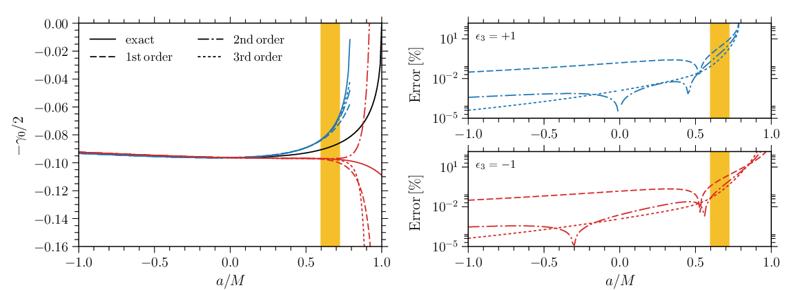
In Figs. 3 and 4, we show the accuracy of this perturbative scheme when used to calculate the real (associated with ) and the imaginary (associated with ) parts of the QNM frequency for . We see that the convergence is rather slow for , although the errors with respect to the exact calculation are typically small otherwise.
V Concluding remarks
As described in the preceding sections, the construction of eikonal limit formulae for the fundamental QNMs of a general post-Kerr spacetime is a straightforward procedure, although the final expressions unavoidably involve some algebraic complexity. The main results of the paper, Eqs. (20) and (21), can be used to produce QNM spectra for any stationary axisymmetric metric that can be written as a perturbation of Kerr. Our illustrative case study of the JP spacetime and the comparison against the “exact” results one can obtain with that metric has helped us to gauge the accuracy of the linear approximation (on top of that related to the use of the eikonal/geodesic approximation).
The validity of our strategy to establish a null test according to the recipe laid out in Section I.1 is also confirmed by numerical simulations, which show that fundamental QNMs with should dominate the ringdown signal in comparable mass black hole mergers [43, 44, 49, 54]. However, in its complete form, the black hole spectroscopy program will require the inclusion of nonequatorial modes (i.e. ), enabling it to handle spinning mergers, where at least the multipole is known to be excited to a significant level33 3 The relative contribution of the asymmetric multipole with respect to the first few modes is a function of the spins of the merging black holes [45, 47]. For small (or exactly zero) spins this multipole is comparable to the mode and much below the mode. This arrangement can be drastically altered in rapidly spinning systems and for certain spin orientations, with the (2, 1) multipole even becoming comparable to the dominant quadrupole (2, 2).. Within our framework, this extension calls for the study of nonequatorial circular photon orbits in non-Kerr spacetimes, and it is an important goal earmarked for follow-up work. In that respect, a great deal of progress in relating nonequatorial photon orbits with QNMs has already been achieved in the context of Kerr black holes [23, 24].
Another key topic that ought to be addressed by future work is the actual detectability and data analysis of QNM signals. Black hole spectroscopy, as a probe for testing the Kerr metric, relies on the extraction of more than one QNM frequency/multipole from the observed gravitational wave signal. This exciting prospect would require a much louder QNM signal (typically a factor boost in the SNR) than those thus far detected by LIGO [11, 12, 13]. Moreover, very recent work [55] suggests that the intrinsic precision of spectroscopy could be affected by the uncertainty in the transition from the merger’s non-linear dynamics to the linear QNM ringdown regime.
Apart from the high SNR/precision requirement, QNM data analysis may also have to face a “confusion problem” when searching for deviations from Kerr. This issue, already familiar from the modeling of extreme mass ratio inspirals in non-Kerr spacetimes [56], has to do with the possibility of misidentifying a true non-Kerr QNM signal with a Kerr one but with a different set of mass and spin parameters. This degeneracy should be broken by the simultaneous observation of the QNM frequency and damping rate and/or the identification of more than one multipole (see e.g. [9, 10]).
As already emphasized, the backbone of our post-Kerr formalism is the eikonal limit association between the spacetime’s light ring and the fundamental QNM. In the case of GR’s garden-variety black holes this connection is intuitively well-established, and performs surprisingly well in approximating the rigorously computed QNMs. Moreover, the fundamental mode is the one dominating the hole’s dynamical response in the time domain.
Since the GW150914 event, however, the light-ring/QNM connection has been the subject of some debate. It has been shown, for instance, that the connection is not as solid as one might think, since it is in principle possible to construct spacetimes where the properties of the wave potential are qualitatively different from those of the geodesic potential for photons [57]. Indeed, a spacetime may have no light rings and still exhibit a QNM ringdown signal. Nevertheless, it should be pointed out that no such counterexample has been constructed for black hole spacetimes resulting from the field equations of a physically sensible modified gravity theory.
The light-ring/QNM connection has also been shown to fail in the context of higher-dimensional Einstein-Lovelock black holes, as a result of the perturbation equations having distinct eikonal limits for different classes of gravitational perturbations [58] (in contrast, the connection has long been known to work for solutions of the higher-dimensional Einstein equations, including Schwarzschild-Tangherlini and Myers-Perry black holes [21]). However, higher-dimensional modifications of gravity are well constrained, and unlikely to give measurable modifications in the context of testing the Kerr solution in astrophysics [59, 6]. Furthermore, the black hole counterexample constructed in [58] is known to exhibit instabilities at large values of the coupling constant of the theory.
The upshot of this discussion is that, although both of the aforementioned counterexamples on the light-ring/QNM connection are interesting and instructive, they have little bearing on our post-Kerr model, since they are not products of consistent modified gravity theories. In the few cases where QNM calculations in such theories do exist (see e.g. [30]), the connection with the circular photon orbit stands as firm as in GR.
Coming from the exactly opposite direction, a series of recent papers [60, 61, 62, 63] uses the light-ring/QNM link to claim indistinguishability between black holes and other horizonless compact objects. Although these two classes of systems are known to support markedly different QNM spectra, they may indeed share the same QNM-like ringdown signal44 4 To our knowledge, this counterintuitive property was first noted by Nollert [64], who replaced the standard Regge-Wheeler potential of Schwarzschild black holes with a potential made of a series of step functions. It had also been seen in the scattering of waves off the potential of compact relativistic stars (see e.g. [19, 65], but until recently this observation was largely overlooked.. This agreement, however, cannot persist for long, since horizonless objects are expected to support a family of slowly damped -modes in the “cavity” formed between the peak of the wave potential and the body’s center (or reflecting surface) [66, 67, 68]. These modes should show up at a later stage of the signal, hence ending any transient similarity with black hole dynamics [69]. It should be noted that the degeneracy in the dynamical response of these objects is partially due to the common exterior Schwarzschild spacetime enforced by Birkhoff’s theorem, so it is conceivable that Kerr black holes may not always share the same ringing signal with horizonless rotating bodies, simply because their light rings are different. The so-called ergoregion instability [70, 71, 72] (which sets in via the same trapped -modes mentioned earlier [73]) may provide another way of lifting the degeneracy between these two types of systems.
As a final remark, it is worth mentioning that the notion of non/post-Kerr light rings (albeit without their connection to QNMs) has already been employed in the context of photon astronomy and the models that are being developed as part of the ongoing effort to produce direct images of our Galactic center supermassive black hole (see e.g. [74]). Although the basic methodology is very different to that of gravitational wave astronomy, the two efforts share the same ultimate goal of probing the physics of the Kerr spacetime.
Acknowledgements.
E.B. was supported by NSF Grants No. PHY-1607130 and AST-1716715, and by FCT contract IF/00797/2014/CP1214/CT0012 under the IF2014 Programme. H.O.S. was supported by NSF Grant No. PHY-1607130. He also thanks Thomas Sotiriou and the University of Nottingham for the hospitality in the final stages of this work. This work was supported by the H2020-MSCA-RISE-2015 Grant No. StronGrHEP-690904.Appendix A Fits of the offset function
In this appendix we present accurate fits for the offset function . In Fig. 5 we show the behavior of as computed from Eq. (1) for modes with . We fitted using the following function, inspired by the classic interatomic Buckingham potential [75]:
| (90) |
The coefficients () for the real and imaginary parts of the leading offset functions (up to ) are listed in Table 1.
As shown in Table 1, the absolute error (defined as ) remains below in the interval . Our results may not be reliable in the near extremal limit (), where the computation of QNMs in computationally challenging and multipole QNM branches exist [24, 26, 76, 77, 78]. The QNM data tables (calculated using Leaver’s continued fraction method) used to obtain are reliable below the theoretical upper bound on the dimensionless spin of astrophysical BHs (the so-called Thorne limit, [79], so our fits should be adequate for astrophysical applications of the present formalism.

| max err. | |||||||
|---|---|---|---|---|---|---|---|
| 2 | 0.1282(0.1381) | 0.4178(0.3131) | 0.6711(0.5531) | 0.5037(0.8492) | 1.8331(2.2159) | 0.7596(0.8544) | 0.023(0.004) |
| 3 | 0.1801(0.1590) | 0.5007(0.3706) | 0.7064(0.6643) | 0.5704(0.6460) | 1.4690(1.8889) | 0.7302(0.6676) | 0.005(0.008) |
| 4 | 0.1974(0.1575) | 0.4982(0.3478) | 0.6808(0.6577) | 0.5958(0.5840) | 1.4380(1.9799) | 0.7102(0.6032) | 0.011(0.009) |
| 5 | 0.2083(0.1225) | 0.4762(0.1993) | 0.6524(0.4855) | 0.6167(0.6313) | 1.4615(3.1018) | 0.6937(0.6150) | 0.016(1.335) |
| 6 | 0.2167(0.1280) | 0.4458(0.1947) | 0.6235(0.5081) | 0.6373(0.6556) | 1.5103(3.0960) | 0.6791(0.6434) | 0.021(0.665) |
| 7 | 0.2234(-15.333) | 0.4116(15.482) | 0.5933(0.0011) | 0.6576(0.3347) | 1.5762(6.6258) | 0.6638(0.2974) | 0.025(0.874) |
Appendix B Circular photon orbits in Kerr
This appendix provides a self-contained discussion of the properties of the equatorial Kerr circular photon orbit. Although this is well known textbook material, we reproduce the calculation as a useful comparison for the more general post-Kerr light ring analysis.
The equatorial Kerr metric in Boyer-Lindquist coordinates reads
| (91) | ||||
| (92) |
Circular motion at the light ring radius simultaneously solves and . We have,
| (93) | ||||
| (94) |
Elimination of leads to
| (95) |
These predict the correct radius for , and also that prograde (retrograde) orbits should have (), but the formula returns an undetermined Schwarzschild limit.
Inserting back into allows us to derive a cubic equation for the impact parameter:
| (96) |
The two real roots of this equation correspond to prograde and retrograde motion.
A different (but completely equivalent) result with a well-defined limit is given by the solution of Eq. (94). This is
| (97) |
where the upper (lower) sign corresponds to prograde (retrograde) motion. Then, Eq. (93) becomes
| (98) |
which is the textbook formula solved by Eq. (6).
The azimuthal orbital frequency at the light ring is given by the turning point formula (30),
| (99) |
We can produce two equivalent expressions using either (95) or (97). The former choice leads to the result
| (100) |
with the inherited (and unattractive) property of a Schwarzschild limit. On the other hand, (97) leads to the textbook formula55 5 The textbook approach is that of Ref. [80]: derive , for circular equatorial motion of a test particle; divide these to obtain the impact parameter ; use this in to arrive at Eq. (7). Note that Ref. [80] skips the details of the complicated calculation of and , which is presented in Chandrasekhar’s book [81]. :
| (101) |
Due to its well defined limit and its “Keplerian” form, this is the preferred formula for .
Appendix C Post-Kerr parameters
In this appendix we list the various coefficients appearing in the post-Kerr analysis of the Lyapunov exponent. Beginning with those appearing in [see Eq. (63)], we have
| (102) |
Next, we list the coefficients of the terms appearing in the expression for [Eq. (66)]. For the -coefficients we have:
| (103) | ||||
| (104) | ||||
For the -coefficients the expression are:
| (106) | ||||
| (107) | ||||
| (108) |
The -coefficients are given by:
| (109) | ||||
| (110) | ||||
| (111) | ||||
| (112) |
Finally, the -coefficients are:
| (113) | ||||
| (114) | ||||
| (115) |
Appendix D The Johannsen-Psaltis expansion coefficients
Here we list the coefficients appearing in the expansions in terms of of the radius of the photon orbit, the impact parameter, and the Lyapunov exponent for the JP spacetime.
First we define the auxiliary coefficients, and , which scale as the mass and the auxiliary coefficient , which scales as the mass to the fourth power.
Taking these definitions into account, the various coefficients have the form
| (116) | |||||
| (117) | |||||
| (118) | |||||
| (119) | |||||
| (120) | |||||
| (121) | |||||
| (122) | |||||
References
- [1] B. P. Abbott et al. (Virgo, LIGO Scientific), Phys. Rev. Lett. 116, 061102 (2016a), arXiv:1602.03837 [gr-qc] .
- [2] B. P. Abbott et al. (Virgo, LIGO Scientific), Phys. Rev. Lett. 116, 241103 (2016b), arXiv:1606.04855 [gr-qc] .
- [3] B. P. Abbott et al. (VIRGO, LIGO Scientific), Phys. Rev. Lett. 118, 221101 (2017), arXiv:1706.01812 [gr-qc] .
- [4] B. P. Abbott et al. (Virgo, LIGO Scientific), Phys. Rev. X6, 041015 (2016c), arXiv:1606.04856 [gr-qc] .
- [5] N. Yunes and X. Siemens, Living Rev. Rel. 16, 9 (2013), arXiv:1304.3473 [gr-qc] .
- [6] E. Berti et al., Class. Quant. Grav. 32, 243001 (2015), arXiv:1501.07274 [gr-qc] .
- [7] B. P. Abbott et al. (Virgo, LIGO Scientific), Phys. Rev. Lett. 116, 221101 (2016d), arXiv:1602.03841 [gr-qc] .
- [8] S. L. Detweiler, Astrophys. J. 239, 292 (1980).
- [9] O. Dreyer, B. J. Kelly, B. Krishnan, L. S. Finn, D. Garrison, and R. Lopez-Aleman, Class. Quant. Grav. 21, 787 (2004), arXiv:gr-qc/0309007 [gr-qc] .
- [10] E. Berti, V. Cardoso, and C. M. Will, Phys. Rev. D73, 064030 (2006), arXiv:gr-qc/0512160 [gr-qc] .
- [11] E. Berti, J. Cardoso, V. Cardoso, and M. Cavaglia, Phys. Rev. D76, 104044 (2007a), arXiv:0707.1202 [gr-qc] .
- [12] E. Berti, A. Sesana, E. Barausse, V. Cardoso, and K. Belczynski, Phys. Rev. Lett. 117, 101102 (2016), arXiv:1605.09286 [gr-qc] .
- [13] K. Belczynski, T. Ryu, R. Perna, E. Berti, T. L. Tanaka, and T. Bulik, (2016), arXiv:1612.01524 [astro-ph.HE] .
- [14] H. Yang, K. Yagi, J. Blackman, L. Lehner, V. Paschalidis, F. Pretorius, and N. Yunes, Phys. Rev. Lett. 118, 161101 (2017), arXiv:1701.05808 [gr-qc] .
- [15] C. V. Vishveshwara, Nature 227, 936 (1970).
- [16] W. H. Press, Astrophys. J. 170, L105 (1971).
- [17] W. L. Ames and K. S. Thorne, ApJ 151, 659 (1968).
- [18] C. J. Goebel, ApJ 172, L95 (1972).
- [19] K. D. Kokkotas and B. G. Schmidt, Living Rev. Rel. 2, 2 (1999), arXiv:gr-qc/9909058 [gr-qc] .
- [20] E. Berti, V. Cardoso, and A. O. Starinets, Class. Quant. Grav. 26, 163001 (2009), arXiv:0905.2975 [gr-qc] .
- [21] V. Cardoso, A. S. Miranda, E. Berti, H. Witek, and V. T. Zanchin, Phys. Rev. D79, 064016 (2009), arXiv:0812.1806 [hep-th] .
- [22] V. Ferrari and B. Mashhoon, Phys. Rev. D30, 295 (1984).
- [23] S. R. Dolan, Phys. Rev. D82, 104003 (2010), arXiv:1007.5097 [gr-qc] .
- [24] H. Yang, D. A. Nichols, F. Zhang, A. Zimmerman, Z. Zhang, and Y. Chen, Phys. Rev. D86, 104006 (2012), arXiv:1207.4253 [gr-qc] .
- [25] H. Yang, F. Zhang, A. Zimmerman, D. A. Nichols, E. Berti, and Y. Chen, Phys. Rev. D87, 041502 (2013a), arXiv:1212.3271 [gr-qc] .
- [26] H. Yang, A. Zimmerman, A. Zenginoğlu, F. Zhang, E. Berti, and Y. Chen, Phys. Rev. D88, 044047 (2013b), [Phys. Rev.D88,044047(2013)], arXiv:1307.8086 [gr-qc] .
- [27] T. Kobayashi, H. Motohashi, and T. Suyama, Phys. Rev. D85, 084025 (2012), arXiv:1202.4893 [gr-qc] .
- [28] T. Kobayashi, H. Motohashi, and T. Suyama, Phys. Rev. D89, 084042 (2014), arXiv:1402.6740 [gr-qc] .
- [29] J. L. Blázquez-Salcedo, L. M. González-Romero, J. Kunz, S. Mojica, and F. Navarro-Lérida, Phys. Rev. D93, 024052 (2016a), arXiv:1511.03960 [gr-qc] .
- [30] J. L. Blázquez-Salcedo, C. F. B. Macedo, V. Cardoso, V. Ferrari, L. Gualtieri, F. S. Khoo, J. Kunz, and P. Pani, Phys. Rev. D94, 104024 (2016b), arXiv:1609.01286 [gr-qc] .
- [31] J. L. Blázquez-Salcedo, F. S. Khoo, and J. Kunz, (2017), arXiv:1706.03262 [gr-qc] .
- [32] V. Cardoso and L. Gualtieri, Phys. Rev. D80, 064008 (2009), [Erratum: Phys. Rev.D81,089903(2010)], arXiv:0907.5008 [gr-qc] .
- [33] C. Molina, P. Pani, V. Cardoso, and L. Gualtieri, Phys. Rev. D81, 124021 (2010), arXiv:1004.4007 [gr-qc] .
- [34] A. Buonanno, L. E. Kidder, and L. Lehner, Phys. Rev. D77, 026004 (2008), arXiv:0709.3839 [astro-ph] .
- [35] E. Berti, V. Cardoso, J. A. Gonzalez, U. Sperhake, and B. Bruegmann, Class. Quant. Grav. 25, 114035 (2008), arXiv:0711.1097 [gr-qc] .
- [36] E. Berti (2014) arXiv:1410.4481 [gr-qc] .
- [37] K. Yagi and L. C. Stein, Class. Quant. Grav. 33, 054001 (2016), arXiv:1602.02413 [gr-qc] .
- [38] T. Johannsen, Phys. Rev. D87, 124017 (2013a), arXiv:1304.7786 [gr-qc] .
- [39] T. Johannsen and D. Psaltis, Phys. Rev. D83, 124015 (2011), arXiv:1105.3191 [gr-qc] .
- [40] V. Cardoso, P. Pani, and J. Rico, Phys. Rev. D89, 064007 (2014), arXiv:1401.0528 [gr-qc] .
- [41] R. Konoplya, L. Rezzolla, and A. Zhidenko, Phys. Rev. D93, 064015 (2016), arXiv:1602.02378 [gr-qc] .
- [42] Z. Younsi, A. Zhidenko, L. Rezzolla, R. Konoplya, and Y. Mizuno, Phys. Rev. D94, 084025 (2016), arXiv:1607.05767 [gr-qc] .
- [43] A. Buonanno, G. B. Cook, and F. Pretorius, Phys. Rev. D75, 124018 (2007), arXiv:gr-qc/0610122 [gr-qc] .
- [44] E. Berti, V. Cardoso, J. A. Gonzalez, U. Sperhake, M. Hannam, S. Husa, and B. Bruegmann, Phys. Rev. D76, 064034 (2007b), arXiv:gr-qc/0703053 [GR-QC] .
- [45] I. Kamaretsos, M. Hannam, S. Husa, and B. S. Sathyaprakash, Phys. Rev. D85, 024018 (2012a), arXiv:1107.0854 [gr-qc] .
- [46] S. Gossan, J. Veitch, and B. S. Sathyaprakash, Phys. Rev. D85, 124056 (2012), arXiv:1111.5819 [gr-qc] .
- [47] I. Kamaretsos, M. Hannam, and B. Sathyaprakash, Phys. Rev. Lett. 109, 141102 (2012b), arXiv:1207.0399 [gr-qc] .
- [48] M. Agathos, W. Del Pozzo, T. G. F. Li, C. Van Den Broeck, J. Veitch, and S. Vitale, Phys. Rev. D89, 082001 (2014), arXiv:1311.0420 [gr-qc] .
- [49] L. London, D. Shoemaker, and J. Healy, Phys. Rev. D90, 124032 (2014), [Erratum: Phys. Rev.D94,no.6,069902(2016)], arXiv:1404.3197 [gr-qc] .
- [50] J. Meidam, M. Agathos, C. Van Den Broeck, J. Veitch, and B. S. Sathyaprakash, Phys. Rev. D90, 064009 (2014), arXiv:1406.3201 [gr-qc] .
- [51] V. Cardoso and L. Gualtieri, Class. Quant. Grav. 33, 174001 (2016), arXiv:1607.03133 [gr-qc] .
- [52] B. Mashhoon, Phys. Rev. D31, 290 (1985).
- [53] A. Maselli, K. Kokkotas, and P. Laguna, Phys. Rev. D93, 064075 (2016), arXiv:1602.01031 [gr-qc] .
- [54] S. Bhagwat, D. A. Brown, and S. W. Ballmer, Phys. Rev. D94, 084024 (2016), [Erratum: Phys. Rev.D95,no.6,069906(2017)], arXiv:1607.07845 [gr-qc] .
- [55] E. Thrane, P. D. Lasky, and Y. Levin, (2017), arXiv:1706.05152 [gr-qc] .
- [56] K. Glampedakis and S. Babak, Class. Quant. Grav. 23, 4167 (2006), arXiv:0510057 [gr-qc] .
- [57] G. Khanna and R. H. Price, Phys. Rev. D95, 081501 (2017), arXiv:1609.00083 [gr-qc] .
- [58] R. A. Konoplya and Z. Stuchlík, (2017), arXiv:1705.05928 [gr-qc] .
- [59] P. Kanti, Int. J. Mod. Phys. A19, 4899 (2004), arXiv:hep-ph/0402168 [hep-ph] .
- [60] V. Cardoso, E. Franzin, and P. Pani, Phys. Rev. Lett. 116, 171101 (2016a), [Erratum: Phys. Rev. Lett.117,no.8,089902(2016)], arXiv:1602.07309 [gr-qc] .
- [61] G. F. Giudice, M. McCullough, and A. Urbano, JCAP 1610, 001 (2016), arXiv:1605.01209 [hep-ph] .
- [62] V. Cardoso, S. Hopper, C. F. B. Macedo, C. Palenzuela, and P. Pani, Phys. Rev. D94, 084031 (2016b), arXiv:1608.08637 [gr-qc] .
- [63] Z. Mark, A. Zimmerman, S. Ming Du, and Y. Chen, (2017), arXiv:1706.06155 [gr-qc] .
- [64] H.-P. Nollert, Phys. Rev. D53, 4397 (1996), arXiv:gr-qc/9602032 [gr-qc] .
- [65] V. Ferrari and K. D. Kokkotas, Phys. Rev. D62, 107504 (2000), arXiv:gr-qc/0008057 [gr-qc] .
- [66] S. Chandrasekhar and V. Ferrari, Proceedings of the Royal Society of London Series A 434, 449 (1991).
- [67] K. D. Kokkotas and B. F. Schutz, Mon. Not. Roy. Astron. Soc. 255, 119 (1992).
- [68] K. D. Kokkotas, Mon. Not. Roy. Astron. Soc. 268, 1015 (1994).
- [69] E. Barausse, V. Cardoso, and P. Pani, Phys. Rev. D89, 104059 (2014), arXiv:1404.7149 [gr-qc] .
- [70] B. F. Schutz and N. Comins, MNRAS 182, 69 (1978).
- [71] N. Comins and B. F. Schutz, Proceedings of the Royal Society of London Series A 364, 211 (1978).
- [72] V. Cardoso, P. Pani, M. Cadoni, and M. Cavaglia, Phys. Rev. D77, 124044 (2008), arXiv:0709.0532 [gr-qc] .
- [73] K. D. Kokkotas, J. Ruoff, and N. Andersson, Phys. Rev. D70, 043003 (2004), arXiv:astro-ph/0212429 [astro-ph] .
- [74] T. Johannsen, Astrophys. J. 777, 170 (2013b), arXiv:1501.02814 [astro-ph.HE] .
- [75] R. A. Buckingham, Proceedings of the Royal Society of London Series A 168, 264 (1938).
- [76] G. B. Cook and M. Zalutskiy, Phys. Rev. D90, 124021 (2014), arXiv:1410.7698 [gr-qc] .
- [77] M. Richartz, Phys. Rev. D93, 064062 (2016), arXiv:1509.04260 [gr-qc] .
- [78] M. Richartz, C. A. R. Herdeiro, and E. Berti, (2017), arXiv:1706.01112 [gr-qc] .
- [79] K. S. Thorne, ApJ 191, 507 (1974).
- [80] J. M. Bardeen, W. H. Press, and S. A. Teukolsky, Astrophys. J. 178, 347 (1972).
- [81] S. Chandrasekhar, The mathematical theory of black holes (Oxford Univ. Press, Oxford, 2002).