Positive approximations of the inverse of fractional powers of SPD M-matrices
Abstract
This study is motivated by the recent development in the fractional calculus and its applications. During last few years, several different techniques are proposed to localize the nonlocal fractional diffusion operator. They are based on transformation of the original problem to a local elliptic or pseudoparabolic problem, or to an integral representation of the solution, thus increasing the dimension of the computational domain. More recently, an alternative approach aimed at reducing the computational complexity was developed. The linear algebraic system , is considered, where is a properly normalized (scalded) symmetric and positive definite matrix obtained from finite element or finite difference approximation of second order elliptic problems in , . The method is based on best uniform rational approximations (BURA) of the function for and natural .
The maximum principles are among the major qualitative properties of linear elliptic operators/PDEs. In many studies and applications, it is important that such properties are preserved by the selected numerical solution method. In this paper we present and analyze the properties of positive approximations of obtained by the BURA technique. Sufficient conditions for positiveness are proven, complemented by sharp error estimates. The theoretical results are supported by representative numerical tests.
1 Introduction
This work is inspired by the recent development in the fractional calculus and its various applications, i.e., to Hamiltonian chaos, [28], anomalous diffusion in complex systems, [2], long-range interaction in elastic deformations, [23], nonlocal electromagnetic fluid flows, [18], image processing, [10]. A more recent impressive examples of anomalous diffusion models in chemical engineering are provided in [19]. Such kind of applications lead to fractional order partial differential equations that involve in general non-symmetric elliptic operators see, e.g. [13]. An important subclass of this topic are the fractional powers of self-adjoint elliptic operators, which are nonlocal but self-adjoint. In particular, the fractional Laplacian [21] describes an unusual diffusion process associated with random excursions. In general, the parabolic equations with fractional derivatives in time are associated with sub-diffusion, while the fractional elliptic operators are related to super-diffusion.
Let us consider the elliptic boundary value problem in a weak form: find such that
| (1) |
where
, and . We assume that has positive measure, in , and is an SPD matrix, uniformly bounded in , i.e.,
| (2) |
for some positive constants and . Also, is a polygonal domain in , , and is a given Lebesgue integrable function on that belongs to the space . Further, the case when does not depend on is referred to as problem in homogeneous media, while the general case models processes in non homogeneous media. The bilinear form defines a linear operator with being the dual of . Namely, for all , where is the pairing between and .
One possible way to introduce , , is through its spectral decomposition, i.e.
| (3) |
Here are the eigenfunctions of , orthonormal in -inner product and are the corresponding positive real eigenvalues. This definition generalizes the concept of equally weighted left and right Riemann-Liouville fractional derivative, defined in one space dimension, to the multidimensional case. There is still ongoing research about the relations of the different definitions and their applications, see, e.g. [3].
The numerical solution of nonlocal problems is rather expensive. The following three approaches (A1 - A3) are based on transformation of the original problem
| (4) |
to a local elliptic or pseudo-parabolic problem, or on integral representation of the solution, thus increasing the dimension of the original computational domain.
The Poisson problem is considered in the related papers refereed bellow, i.e.
- A1
Extension to a mixed boundary value problem in the semi-infinite cylinder
A “Neumann to Dirichlet” map is used in [6]. Then, the solution of fractional Laplacian problem is obtained by where is a solution of the equation
where satisfies the boundary conditions of (1) ,
as well as
It is shown that the variational formulation of this equation is well posed in the related weighted Sobolev space. The finite element approximation uses the rapid decay of the solution in the direction, thus enabling truncation of the semi-infinite cylinder to a bounded domain of modest size. The proposed multilevel method is based on the Xu-Zikatanov identity [27]. The numerical tests for and confirm the theoretical estimates of almost optimal computational complexity.
- A2
Transformation to a pseudo-parabolic problem
The problem (1) is considered in [25, 26] assuming the boundary condition
which ensures , . Then the solution of fractional power diffusion problem can be found as
where , is the solution of pseudo-parabolic equation
and . Stability conditions are obtained for the fully discrete schemes under consideration. A further development of this approach is presented in [16] where the case of fractional order boundary conditions is studied.
- A3
Integral representation of the solution
The following representation of the solution of (1) is used in [4]:
Among others, the authors introduce an exponentially convergent quadrature scheme. Then, the approximate solution of only involves evaluations of , where is related to the current quadrature node, and where and stand for the identity and the finite element stiffness matrix corresponding to the Laplacian. The computational complexity of the method depends on the number of quadrature nodes. For instance, the presented analysis shows that approximately 50 auxiliary linear systems have to be solved to get accuracy of the quadrature scheme of order for . A further development of this approach is available in [5], where the theoretical analysis is extended to the class of regularly accretive operators.
An alternative approach is applied in [11] where a class of optimal solvers for linear systems with fractional power of symmetric and positive definite (SPD) matrices is proposed. Let be a normalized SPD matrix generated by a finite element or finite difference approximation of some self-adjoint elliptic problem. An efficient method for solving algebraic systems of linear equations involving fractional powers of the matrix is considered, namely for solving the system
| (5) |
The fractional power of SPD matrix , similarly to the infinite dimensional counterpart , is expressed through the spectral representation of through the eigenvalues and eigenvectors of , assuming that the eigenvectors are -orthonormal, i.e. and . Then , , where the matrices and are defined as and , , and the solution of can be expressed as
| (6) |
Instead of the system (5), one can solve the equivalent system with an integer. Then the idea is to approximately evaluate using a set of equations involving inversion of and , for . The integer parameter is the number of partial fractions of the best uniform rational approximation (BURA) of on the interval . One can observe that the algorithm of [4], see A3, can be viewed as a particular rational approximation of . It is also important, that in certain sense the results from [11] are more general, and are applicable to a wider class of sparse SPD matrices.
Assuming that is a large-scale matrix, the computational complexity of the discussed methods for numerical solution of fractional diffusion problems is substantially high. Then, the parallel implementation of such methods for real life problems is an unavoidable topic. In this context, there are some serious advantages of the last two approaches, see e.g., in [8].
The maximum principles are among the major qualitative properties of the elliptic or parabolic operators/PDEs. In general, to solve PDEs we use some numerical method, and it is a natural requirement that such qualitative properties are preserved on the discrete level. Most of the studies which deal with such topics give sufficient conditions for the discretization parameters in order to guarantee the certain maximum principle. It is easily see, that under certain such assumptions, the solutions of (A1) and (A3) satisfy certain maximum principle. In this paper, we study positive approximations of , obtained by BURA technique introduced in [11], under rather general assumptions for the normalized SPD matrix .
The rest of the paper is organized as follows. In Section 2 we provide a brief introduction to the topic of monotone matrices including some basic properties of the M-matrices and their relations to FEM discretization of elliptic PDEs. Sufficient conditions for positive approximations of the inverse of a given SPD matrix, based on BURA technique are presented in Section 3. The analysis in Section 4 is devoted to a class of best rational approximations of , that satisfy such sufficient conditions. Sharp error estimates for a class of BURA approximations are also included in this section. Some numerical tests and short concluding remarks are given at the end.
2 Monotone matrices and SPD M-matrices
The maximum principles are some of the most useful properties used to solve a wide range of problems in the PDEs. For instance, their use is often essential to study the uniqueness and necessary conditions of solvability, approximation and boundedness of the solution, as well as, for quantities of physical interest like maximum stress, torsional stiffness, electrostatic capacity, charge density etc. Under certain regularity conditions, a classical maximum principle for elliptic problems reads as follows. Suppose that in , then a nonnegative maximum is attained at the boundary . Let us assume additionally that in . Then the positivity preserving property holds, that is, for or .
To solve PDEs we use some numerical methods, and it is a natural requirement that such qualitative properties are preserved on the discrete level. Most of the papers which deal with this topic give sufficient conditions for the discretization parameters in order to guarantee the certain maximum principle. For instance, when FEM is applied, the related results are usually described in terms of properties of the related mass and stiffness matrices.
Definition 2.1
A real square matrix is called monotone if for all real vectors , implies , where is in element-wise sense.
The next property is sometimes used as an alternative definition.
Proposition 2.2
Let be a real square matrix. is monotone if and only if .
Definition 2.3
The class of Z-matrices are those matrices whose off-diagonal entries are less than or equal to zero. Let be a real Z-matrix, then is a non-singular M-matrix if every real eigenvalue of is positive. A symmetric M-matrix is sometimes called a Stieltjes matrix.
The M-matrices are among most often used monotone matrices. They arise naturally in some discretizations of elliptic operators.
Let be an SPD matrix obtained after FEM approximation of (1) by linear triangle elements. Let us assume also that is discretized by a nonobtuse triangle mesh , and the coefficients and are piecewise constants on the triangles . Then can be assembled by the element matrices
where is the element stiffness matrix and is the element mass matrix. Subject to a scaling factor, the off diagonal elements of the symmetric and positive semidefinite matrix are equal to some of , , where are the nonobtuse angles of the triangle . Imposing the boundary conditions we get that the global stiffness matrix is SPD M-matrix. The element mass matrix is positive diagonal matrix if a proper quadrature formula is applied. A similar result can be obtained by the standard diagonalization known as lumping the mass. Then, the global mass matrix is positive diagonal matrix and is SPD M-matrix. A more general considerations of this kind are available in [15] including the case of coefficient anisotropy as well as the nonconforming linear finite elements. Similar representations of the element mass and stiffness matrices are derived if is discretized by a nonobtuse tetrahedral mesh . We get again that is again SPD M-matrix, see e.g., [14].
Remark 2.4
Not all monotone matrices are M-matrices, and the sum of two monotone matrices is not always monotone. The next examples prove these statements.
Example 2.5
- E1.1
is not M-matrix, but and therefore is monotone.
- E1.2
is a sum of two monotone matrices, but and therefore is not monotone.
In what follows, we study positive approximations of for a given normalized SPD M-matrix . It follows straightforwardly that the inverse of each such approximation will approximate in the class of monotone functions.
3 Positive approximations of the inverse of SPD M-matrices
Explicit computation and memory storage of the fractional power in (5) for large-scale problems is expensive and impractical. Even when is sparse, is typically dense. Therefore, we study possible positive approximations of the action of based solely on the information of . For this purpose, we consider the class of rational functions
fix a positive integer , and search for an appropriate candidate in it, that approximates well the univariate function on the unit interval . Note that, due to the normalization of , this interval covers the spectrum of ,
Definition 3.1
Let , and . The minimizer of the problem
| (7) |
will be called -Best Uniform Rational Approximation (-BURA). Its error will be denoted by
Based on classical Spectral Theory arguments (see [11, Theorem 2.1]), the univariate approximation error is an upper bound for the multivariate relative error for the corresponding matrix-valued BURA approximation of the exact solution in (6). Here, can be arbitrary, and the Krylov norms are defined via standard energy dot product, i.e. .
Proposition 3.2
Let be an SPD matrix with eigenvalues . Let be the -BURA for given . Then,
| (8) |
For the practical computation of we use the partial fraction decomposition of , which is of the form
| (9) |
provided all has no complex poles and the real ones are all of multiplicity 1. Later, we will see that for and the above assumption on the poles of holds true for any . Furthermore, in all our numerical experiments with various and the assumption always remains valid. Hence, it does not seem to restrict the application range of the proposed method. On the other hand, under (9) the approximate solution
| (10) |
of can be efficiently numerically computed via solving several linear systems, that involve and its diagonal variations , for .
Definition 3.3
A real symmetric matrix is said to be doubly nonnegative if it is both positive definite, and entrywise nonnegative.
Our first goal is to analyze under what conditions on the coefficients and the poles in (9), the matrix remains doubly nonnegative. Clearly the matrix is symmetric whenever is, so the main investigations are on assuring . The following proposition contains sufficient conditions for positivity.
Proposition 3.4
If is a normalized SPD M-matrix, , , , and (entrywise), then in (10) is doubly nonnegative. Proof: Since , equation (10) is simplified to
For every , the matrix is an SPD M-matrix, as and the
diagonal elements increase their values,
i.e. become stronger dominant.
Hence, .We have , thus , , as each entry of is a
sum of nonnegative summands. Finally, a linear combination of positively scaled doubly nonnegative matrices is also a
doubly nonnegative matrix.
Note that, when applying pure polynomial approximation techniques for on like in [12], there is practically no chance to come up with a positive approximation of . First of all, such an approximant is a linear combination of positive degrees of and in particular itself appears with a nonzero coefficient. This matrix has non-positive off-diagonal entries. Furthermore, it was numerically observed that the coefficient sequence in the linear combination is sign alternating. Hence, the proposed -BURA approach seems the right and most natural tool for constructing positive approximations of , or alternatively, monotone approximations of . Another disadvantage of the former approach is the restriction on to be well-separated from zero, which is also a restriction on the condition number of .
4 Analysis of a class of best rational approximations of fractional power of SPD M-matrices
Among all various classes of best rational approximations, the diagonal sequences of the Walsh table of , are studied in greatest detail [20, 9, 24, 22]. There is an existence and uniqueness of the BURA elements for all and . The distribution of poles, zeros, and extreme points of those elements plays a central role in asymptotic convergence analysis, when , thus is well known. In this section, we show that the above diagonal class perfectly fits within our positive approximation framework.
First, we collect some preliminary results that will be later needed for the proof of the main theorem. The following characterization lemma, which we state here without proof, is vital for our further investigations.
Lemma 4.1
[22, Lemma 2.1] Let and .
- (a)
The best rational approximant is of exact numerator and denominator degree .
- (b)
All zeros and poles of lie on the negative half-axis and are interlacing; i.e., with an appropriate numbering we have
(11) - (c)
The error function has exactly extreme points on , and with an appropriate numbering we have
(12) (13)
The next lemma builds a bridge between the fractional decompositions of and .
Lemma 4.2
Let , , and
Then
| (14) |
Proof: The second part of (14) follows directly from
For the first part, we combine the above identity with (12) and (13)
The proof of the lemma is completed.
Our last lemma provides an asymptotic bound on . The proof can be found in [24].
Lemma 4.3
Now, we are ready to formulate and prove our main result.
Theorem 4.4
Let and . For every normalized SPD M-matrix and every , the matrix is doubly nonnegative and for all
| (15) |
Proof:
Based on the results in Lemma 4.1, we can quickly derive . For this purpose, we study the sign pattern of and and assure the applicability of Proposition 3.4. From (11) we know that all the poles are real, negative, and of multiplicity 1. The same holds true for the zeros . Since is continuous on , the function changes its sign times - at each zero and at each pole . In Lemma 4.2, we have already computed that , thus, due to interlacing, at each pole we have
Since and , from Lemma 4.2 it follows that and . Hence, Proposition 3.4 gives rise to .
The error estimate (15) is a direct corollary of Proposition 3.2 and Lemma 4.3.
Some remarks are in order. For any fixed , the relative error (15) decays exponentially as
with order . When the relative error decays linearly independently of
, since . It is straightforward to extend the coefficient
correspondence (14) to for any ,
such that . Therefore, a necessary condition for Proposition 3.4 to be applicable is the sequence
to have constant sign. Due to the proof of Theorem 4.4, it implies that zeros and
poles of should be interlacing, thus . Furthermore (see [11, (20)])
the following identity always holds true
Hence, another necessary condition for applicability of Proposition 3.4 is . Combining all derived constraints, we observe that could be represented as a sum of doubly nonnegative matrices only if and , meaning that we are left with the admissible triples
In [22] it is remarked that for the case it cannot be theoretically excluded that one root and one pole of the 2-BURA lie outside of . For the case we can show that , thus the assumptions of the proposition are again violated. In conclusion, the triple , investigated in Theorem 4.4 is the unique choice of parameters for which one can prove positiveness of the approximation using Proposition 3.4.
5 Numerical tests
The main goal of the numerical tests is to illustrate the positive properties of the proposed approximations of inverse of fractional powers of SPD M-matrices. Complementary, we provide a short discussion related to some interpretations of the results from Section 4 in the case of fractional diffusion problems.
The test problems are in 1D. In this case we are able easier to compute the exact solutions of linear systems with fractional powers of the corresponding tridiagonal matrix. Note that this does not cause restrictions to the derived conclussions. As it was shown in [11], if , some PCG solver of optimal complexity (e.g., BoomerAMG) can be utilized for efficient solution of the arising sparse linear systems, fully preserving the accuracy and efficiency of the composite algorithm.
We consider fractional powers of the Poisson’s equation on the unit interval with Dirichlet boundary conditions:
| (16) |
On a uniform grid with mesh parameter , using central finite differences, the operator is approximated by the matrix , which in turn can be rewritten as
| (17) |
The matrix is a normalized, SPD M-matrix, which eigenvectors and eigenvalues are explicitly known:
We approximate by and, due to Theorem 4.4, the relative error is bounded by an -dependent constant.
Corollary 5.1
Let be the exact solution of the discretized fractional Poisson’s equation . Let be 1-BURA and denote by . Then
Proof: Indeed, let and . Applying
where is the condition number of , we derive
| (18) |
The result follows from (15) for .
Due to Corollary 5.1, we can compute the minimal degree that guarantees for every given pair . Such an error analysis is outside of the scope of this
paper, so we will not further elaborate on it.
| 0.25 | 2.8676e-5 | 9.2522e-6 | 3.2566e-6 |
| 0.50 | 2.6896e-4 | 1.0747e-4 | 4.6037e-5 |
| 0.75 | 2.7162e-3 | 1.4312e-3 | 7.8966e-4 |
In our numerical experiments, we choose and . The square root of an M-matrix is again an M-matrix [1] and it is easy to check that is also an M-matrix. Therefore, all considered are M-matrices, their inverse matrices are doubly nonnegative (but dense!), and constructing computationally cheep approximants within the same class is of great practical importance. The univariate error estimates for the above choice of parameters are summarized in Table 1. Note that each of them satisfies the inequality (15) even without introducing the low-order term in the right-hand-side. A modified Remez algorithm is used for the derivation of [17, 7].
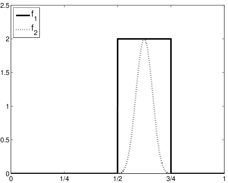
For in (4) we take two different positive functions, supported on the interval . The first one is piecewise constant and discontinuous, while the second one is a cubic spline function, corresponding to the Irwin-Hall distribution. Together with the exact discretized solutions , they are illustrated on Fig. 1.
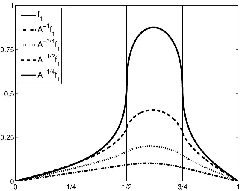
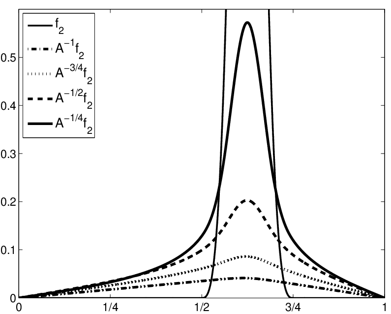


We consider mesh parameters , . On Fig. 2 the corresponding approximants , , of are plotted. As suggested by Corollary 5.1, fails to approximate well on a fine grid for smaller and (see , ). For larger , the exponential growth of the relative error with is less significant, as it is of order , thus when all the three approximants, corresponding to follow closely the graph of . On Fig. 3 and in Table 2 we numerically confirm the asymptotic behavior of the relative error from Corollary 5.1.


| 6.3e-5 | 1.2e-4 | 7.5e-5 | 1.9e-4 | 3.1e-4 | 1.0e-4 | 8.5e-4 | 3.5e-4 | 2.1e-4 | |
| 6.8e-4 | 2.1e-4 | 1.2e-4 | 9.3e-4 | 6.2e-4 | 2.6e-4 | 3.0e-4 | 7.3e-4 | 1.9e-4 | |
| 4.9e-3 | 9.9e-4 | 2.2e-4 | 3.2e-3 | 1.3e-3 | 5.5e-4 | 1.6e-3 | 1.0e-3 | 6.6e-5 | |
| 1.2e-2 | 4.9e-3 | 1.0e-3 | 5.0e-3 | 2.4e-3 | 1.0e-3 | 2.7e-3 | 6.7e-4 | 4.4e-4 | |
| 3.7e-2 | 9.6e-3 | 4.9e-3 | 5.6e-3 | 1.3e-3 | 1.2e-3 | 8.2e-4 | 1.3e-3 | 1.1e-3 | |
| 2.1e-2 | 3.6e-2 | 9.5e-3 | 2.4e-2 | 8.8e-3 | 1.4e-3 | 5.8e-3 | 3.0e-3 | 1.5e-3 | |
| 1.9e-1 | 2.3e-2 | 3.6e-2 | 4.2e-2 | 1.4e-2 | 8.9e-3 | 1.6e-3 | 9.9e-4 | 4.3e-4 | |
The sufficient conditions from Proposition 3.4 hold true for the cases under consideration. This means that positivity of all considered approximations is guaranteed. Therefore, the discrete maximum principle is always inherited. The presented numerical results are fully aligned with the theory. What is very important is the numerical robustness of positivity with respect to both accuracy parameters and which is confirmed for all . Even in the case of lower accuracy, we do not observe any oscillations. The monotonicity preservation of the data is clearly expressed, capturing their geometrical shape.
6 Concluding remarks
This study is inspired by some quite recent results in the numerical methods for fractional diffusion problems. In the Introduction, we discussed three methods based on reformulation of the original nonlocal problem into local (elliptic, pseudo parabolic, and integral) problems. In all cases, the cost is in the increased dimension of computational domain from to .
Our approach is based on best uniform rational approximations of , . The primal motivation is to reduce the computational complexity. A next important step is made in this paper. Here, we provide sufficient conditions to guarantee positive approximation of the inverse of fractional powers of normalized SPD M-matrices. Therefore, we get a numerical method which preserves the maximum principle. The presented numerical results clearly confirm the monotone behaviour of the solution, without any observed oscillations. Further research has to be devoted to the topic of accuracy of mass conservation.
The currently available methods and algorithms for numerical solution of boundary value problems with fractional power of elliptic operators have a quite different nature. A serious theoretical and experimental study is required to get a comparative analysis of their advantages and disadvantages for particular classes of problems. For instance, the error analysis is in different functional spaces assuming different conditions for smoothness. The comparison of the computational complexity is also an open question.
As a part of our analysis, Theorem 1 provides a sharp error estimates for the 1-BURA based approximations . Then, at the beginning of Section 5, we showed how this result can be used to derive relative error estimates of the numerical solution of fractional order elliptic problems in . The numerical tests are well aligned with this theoretical estimates. The presented approach has a strong potential for further development addressing different pairs of functional spaces in the relative error estimates, varying the smoothness assumptions, for .
In addition, a lot of new numerical tests are needed to evaluate/confirm/compare the computational efficiency for more realistic towards real-life large-scale super diffusion problems.
References
- [1] G. Alefeld and N. Schneider. On square roots of M-matrices. Linear Algebra and its Applications, 42:119–132, 1982.
- [2] O. G. Bakunin. Turbulence and Diffusion: Scaling Versus Equations. Springer Science & Business Media, 2008.
- [3] P. W. Bates. On some nonlocal evolution equations arising in materials science. Nonlinear dynamics and evolution equations, 48:13–52, 2006.
- [4] A. Bonito and J. Pasciak. Numerical approximation of fractional powers of elliptic operators. Mathematics of Computation, 84(295):2083–2110, 2015.
- [5] A. Bonito and J. Pasciak. Numerical approximation of fractional powers of regularly accretive operators. IMA J Numer Anal, pages drw042v1–drw042, 2016.
- [6] L. Chen, R. Nochetto, O. Enrique, and A. J. Salgado. Multilevel methods for nonuniformly elliptic operators and fractional diffusion. Mathematics of Computation, 85:2583–2607, 2016.
- [7] E. W. Cheney and M. J. D. Powell. The differential correction algorithm for generalized rational functions. Constructive Approximation, 3(1):249–256, 1987.
- [8] R. Ciegis, V. Starikovicius, and S. Margenov. On parallel numerical algorithms for fractional diffusion problems. Third NESUS Workshop, COST IC1305, October 2016.
- [9] T. Ganelius. Rational approximation of on . Anal. Math., 5:19–33, 1979.
- [10] G. Gilboa and S. Osher. Nonlocal operators with applications to image processing. Multiscale Modeling & Simulation, 7(3):1005–1028, 2008.
- [11] S. Harizanov, R. Lazarov, S. Margenov, P. Marinov, and Y. Vutov. Optimal solvers for linear systems with fractional powers of sparse SPD matrices. submitted, posted as arXiv:1612.04846v1, December 2016.
- [12] S. Harizanov, S. Margenov, P. Marinov, and Y. Vutov. Volume constrained 2-phase segmentation method utilizing a linear system solver based on the best uniform polynomial approximation of . Journal of Computational and Applied Mathematics, 310:115–128, 2017.
- [13] A. Kilbas, H. Srivastava, and J. Trujillo. Theory and Applications of Fractional Differential Equations. Elsevier, Amsterdam, 2006.
- [14] N. Kosturski and S. Margenov. MIC(0) preconditioning of 3D FEM problems on unstructured grids: conforming and non-conforming elements. J. Comp. Appl. Math., 226(2):288–297, 2009.
- [15] J. Kraus and S. Margenov. Robust Algebraic Multilevel Methods and Algorithms, volume 5. de Gruyter, 2009.
- [16] R. Lazarov and P. Vabishchevich. A numerical study of the homogeneous elliptic equation with fractional order boundary conditions. submitted, posted as arXiv:1702.06477v1, February 2017.
- [17] P. G. Marinov and A. S. Andreev. A modified Remez algorithm for approximate determination of the rational function of the best approximation in Hausdorff metric. Comptes rendus de l’Academie bulgare des Scieces, 40(3):13–16, 1987.
- [18] B. McCay and M. Narasimhan. Theory of nonlocal electromagnetic fluids. Archives of Mechanics, 33(3):365–384, 1981.
- [19] R. Metzler, J.-H. Jeon, A. G. Cherstvy, and E. Barkai. Anomalous diffusion models and their properties: non-stationarity, non-ergodicity, and ageing at the centenary of single particle tracking. Physical Chemistry Chemical Physics, 16(44):24128–24164, 2014.
- [20] D. J. Newman. Rational approximation to . The Michigan Mathematical Journal, 11(1):11–14, 1964.
- [21] C. Pozrikidis. The Fractional Laplacian. Chapman and Hall/CRC, 2016.
- [22] E. B. Saff and H. Stahl. Asymptotic distribution of poles and zeros of best rational approximants to on . In "Topics in Complex Analysis", Banach Center Publications, volume 31. Institute of Mathematics, Polish Academy of Sciences, Warsaw, 1995.
- [23] S. A. Silling. Reformulation of elasticity theory for discontinuities and long-range forces. Journal of the Mechanics and Physics of Solids, 48(1):175–209, 2000.
- [24] H. Stahl. Best uniform rational approximation of on . Bulletin of the American Mathematical Society, 28(1):116–122, 1993.
- [25] P. N. Vabishchevich. Numerical solving the boundary value problem for fractional powers of elliptic operators. CoRR, abs/1402.1636, 2014.
- [26] P. N. Vabishchevich. Numerically solving an equation for fractional powers of elliptic operators. Journal of Computational Physics, 282:289–302, 2015.
- [27] J. Xu and L. Zikatanov. The method of alternating projections and the method of subspace corrections in Hilbert space. Journal of the American Mathematical Society, 15(3):573–597, 2002.
- [28] G. M. Zaslavsky. Chaos, fractional kinetics, and anomalous transport. Physics Reports, 371(6):461–580, 2002.