跳到论文正文
W Papers独立论文阅读器 arXiv:1706.06712 论文正文 计算阅读时间 · 0%
引用这篇论文根据当前论文元数据生成,正式投稿前建议核对。


License: arXiv.org perpetual non-exclusive license
arXiv:1706.06712v3 [math.NT] 30 May 2022

Integral points on Markoff type cubic surfaces

Amit Ghosh Address: Oklahoma State University
Stillwater, OK 74078, USA
Current address: Email address: ghosh@okstate.edu
and Peter Sarnak Address: Institute for Advanced Study and Princeton University
Princeton, NJ 08540, USA
Current address: Email address: sarnak@math.ias.edu
Abstract.

For integers kk, we consider the affine cubic surface VkV_{k} given by M⁡(𝐱)=x12+x22+x32−x1​x2​x3=kM({\bf x})=x_{1}^{2}+x_{2}^{2}+x_{3}^{2}-x_{1}x_{2}x_{3}=k. We show that for almost all kk the Hasse Principle holds, namely that Vk​(ℤ)V_{k}(\mathbb{Z}) is non-empty if Vk​(ℤp)V_{k}(\mathbb{Z}_{p}) is non-empty for all primes pp, and that there are infinitely many kk’s for which it fails. The Markoff morphisms act on Vk​(ℤ)V_{k}(\mathbb{Z}) with finitely many orbits and a numerical study points to some basic conjectures about these “class numbers” and Hasse failures. Some of the analysis may be extended to less special affine cubic surfaces.

1. Introduction

Little is known about the values at integers assumed by affine cubic forms FF in three variables. Unless otherwise stated, by an affine form ff in nn-variables we mean f∈ℤ⁡[x1,…,xn]f\in\mathbb{Z}[x_{1},\ldots,x_{n}] whose leading homogeneous term f0f_{0} is non-degenerate(1) (1)  (1)  that is it cannot be transformed to a polynomial of fewer than nn variables by a linear change of variables. and such that f−kf-k is (absolutely) irreducible for all constants kk. For k∈ℤk\in\mathbb{Z} set

(1.1) Vk,F={𝐱=(x1,x2,x3):F⁡(𝐱)=k},V_{k,F}=\{{\bf x}=(x_{1},x_{2},x_{3}):\ F({\bf x})=k\},

and 𝔳F​(k):=|Vk,F​(ℤ)|\mathfrak{v}_{F}(k):=|V_{k,F}(\mathbb{Z})|. The basic question is for which kk is Vk,F​(ℤ)≠∅V_{k,F}(\mathbb{Z})\neq\emptyset, or more generally infinite or Zariski dense in Vk,FV_{k,F} ?

A prime example is F=SF=S, the sum of three cubes:

(1.2) S⁡(x1,x2,x3)=x13+x23+x33.S(x_{1},x_{2},x_{3})=x_{1}^{3}+x_{2}^{3}+x_{3}^{3}.

There are obvious local congruence obstructions, namely that Vk,S​(ℤ)=∅V_{k,S}(\mathbb{Z})=\emptyset if k≡4​or​ 5​(mod​ 9)k\equiv 4\ \text{or}\ 5\,({\rm mod}\,9), but beyond that it is possible that the answers to all three questions is yes for all the other kk’s, which we call the admissible values (see [Mor69], [CV94]). It is known that strong approximation in its strongest form fails for Vk,S​(ℤ)V_{k,S}(\mathbb{Z}); the global obstruction coming from an application of cubic reciprocity ([Cas85], [HB92], [CTW12]). Moreover, [Leh56] and [Beu95] show that V1,S​(ℤ)V_{1,S}(\mathbb{Z}) is Zariski dense in V1,SV_{1,S}.

The case when the cubic polynomial F⁡(x1,x2,x3)F(x_{1},x_{2},x_{3}) factors into linear factors can be studied algebraically using divisor theory, and is apparently quite different to our irreducible FF. If FF is the split norm form N⁡(𝐱)=x1​x2​x3N({\bf x})=x_{1}x_{2}x_{3}, then every Vk,NV_{k,N} is non-empty, and for kk non-zero, 𝔳N​(k)\mathfrak{v}_{N}(k) is finite and is a divisor function.

For a ℚ\mathbb{Q}-anistropic torus given by N⁡(𝐱)=N​mK/ℚ​(α1​x1+α2​x2+α3​x3)N({\bf x})={Nm}_{K/\penalty\mathbb{Q}}(\alpha_{1}x_{1}+\alpha_{2}x_{2}+\alpha_{3}x_{3}), where α1,α2,α3\alpha_{1},\,\alpha_{2},\,\alpha_{3} is a ℤ\mathbb{Z}-basis of an order in a cubic number field KK, the Dirichlet Unit Theorem coupled with the action 𝐰→u​𝐰{\bf w}\rightarrow u{\bf w} of the unit group on the homogeneous space and the theory of divisors, allows for the study of Vk,N​(ℤ)V_{k,N}({\mathbb{Z}}). It consists of a finite number 𝔥N​(k)\mathfrak{h}_{N}(k) of orbits (putting 𝔥N​(k)=𝔳N​(k)=0\mathfrak{h}_{N}(k)=\mathfrak{v}_{N}(k)=0 if Vk,N=∅V_{k,N}=\emptyset), is infinite if it is non-empty and is Zariski dense if KK is totally real. The dependence of 𝔥N​(k)\mathfrak{h}_{N}(k) on kk is subtle, especially if the class number HH of the order is not one. Most kk’s are not represented; in fact [Odo77] shows that

(1.3) |{|k|≤X:𝔳N​(k)≠0}|∼1H|{|k|≤X:k​admissible}|∼C​X​(log⁡X)−23,\big|\{|k|\leq X:\mathfrak{v}_{N}(k)\neq 0\}\big|\sim\frac{1}{H}\big|\{|k|\leq X:k\ \text{admissible}\}\big|\sim CX(\log X)^{-\frac{2}{3}}\,,

as X→∞X\to\infty . The question of the density of Hasse failures for norms of elements in a number field KK is studied in [BN16].

To measure the richness of representations by ff, we say that ff is perfect if Vk,f​(ℤ)V_{k,f}(\mathbb{Z}) is Zariski dense in Vk,fV_{k,f} for all but finitely many admissible kk’s; we say it is almost perfect if the same holds for almost all admissible kk (in the sense of natural density); and ff is full if 𝔳f​(k)→∞\mathfrak{v}_{f}(k)\to\infty as k→∞k\to\infty for almost all admissible kk’s. For an affine form, it follows from [LW54] and [Sch76] that the admissible kk’s are given in terms of a congruence condition as in the case of SS.

Much more is known about cubic forms in the “subcritical” case of forms in four or more variables or diagonal forms f=x1a1+…+xbabf=x_{1}^{a_{1}}+\ldots+x_{b}^{a_{b}} with ∑j=1baj−1>1\sum_{j=1}^{b}a_{j}^{-1}>1 and b≥3b\geq 3 (see [Hoo16], [VW02], [Bro15] for example) and in the “super-critical" case of two variables ([FZ14]). The basic analytic feature in the subcritical case is that the average number of representations of kk is kδ​(log⁡k)Ak^{\delta}(\log k)^{A} for some δ>0\delta>0, while in the critical case, δ=0\delta=0. If ff is a cubic polynomial, n≥10n\geq 10 and f0f_{0} is nonsingular then ff is perfect ([BHB09])(2) (2)  (2)  They show that |Vk,f​(ℤ)|=∞|V_{k,f}(\mathbb{Z})|=\infty for kk admissible from an asymptotic count which is flexible enough to deduce that Vk,f​(ℤ)V_{k,f}(\mathbb{Z}) is Zariski dense in Vk,fV_{k,f}.. In a recent paper [Hoo16], it is shown that if f=f0f=f_{0} and is nonsingular with n≥5n\geq 5, then ff is full, while conditional on the Riemann Hypothesis for certain Hasse-Weil LL-functions, the same is true for n≥4n\geq 4. Moreover, it is conjectured there that any such ff with n≥4n\geq 4 is perfect. For cubic ff in two variables (supercritical case) the celebrated theorems ([Thu09], [Sie29]) assert that Vk,f​(ℤ)V_{k,f}(\mathbb{Z}) is finite and moreover only for very few of the admissible kk’s is Vk,f​(ℤ)V_{k,f}(\mathbb{Z}) non-empty ([Sch87]).

Returning to the critical dimension n=3n=3 for affine cubic forms, there are well-known examples of FF which are not perfect, see ([Mor53], [CG66])(3) (3)  (3)  The projective cubic surface for [CG66], namely F⁡(x1,x2,x3)=10​x43F(x_{1},x_{2},x_{3})=10x_{4}^{3} with F⁡(x1,x2,x3)=5​x13+12​x23+9​x33F(x_{1},x_{2},x_{3})=5x_{1}^{3}+12x_{2}^{3}+9x_{3}^{3}, fails the Hasse principle over ℚ\mathbb{Q}; from which it follows that Vk,F​(ℤ)V_{k,F}(\mathbb{Z}) fails the Hasse principle over ℤ\mathbb{Z} for k=10​w3k=10w^{3}. There are many other such projective cubic surfaces over ℚ\mathbb{Q} (see Sec. 4 of [Bro17]). and also our example of MM below; however it is possible that FF is always full (see the discussion at the end of the Introduction).

This paper is concerned with F=MF=M where

(1.4) M⁡(𝐱)=x12+x22+x32−x1​x2​x3.M({\bf x})=x_{1}^{2}+x_{2}^{2}+x_{3}^{2}-x_{1}x_{2}x_{3}.

The affine cubic surface V0,M​(ℤ)V_{0,M}(\mathbb{Z}) was studied by Markoff ([Mar79], [Mar80]); the points (x1,x2,x3)∈V0,M​(ℤ)(x_{1},x_{2},x_{3})\in V_{0,M}(\mathbb{Z}) with xj∈ℕx_{j}\in\mathbb{N} being essentially the “Markoff triples” . The reason that one can study V0,M​(ℤ)V_{0,M}(\mathbb{Z}), or more generally Vk,M​(ℤ)V_{k,M}(\mathbb{Z}) is that there is a descent group action albeit non-linear. The Vieta involutions 𝒱j\mathcal{V}_{j} with 𝒱1​(x1,x2,x3)=(x2​x3−x1,x2,x3)\mathcal{V}_{1}(x_{1},x_{2},x_{3})=(x_{2}x_{3}-x_{1},x_{2},x_{3}) and similarly for 𝒱2\mathcal{V}_{2}, 𝒱3\mathcal{V}_{3}, preserve MM, as do permutations of the xjx_{j}’s and switching the signs of two of the xjx_{j}’s. We denote by Γ\Gamma the group of polynomial affine transformations generated as above. Then, Γ\Gamma preserves Vk,M​(ℤ)V_{k,M}(\mathbb{Z}) and except for the case of the Cayley cubic with k=4k=4 (see Sec. 4.3), Vk,M​(ℤ)V_{k,M}(\mathbb{Z}) decomposes into a finite number 𝔥M​(k)\mathfrak{h}_{M}(k) of Γ\Gamma-orbits. For example, if k=0k=0, then 𝔥M​(0)=2\mathfrak{h}_{M}(0)=2 corresponds to the orbits of (0,0,0)(0,0,0) and (3,3,3)(3,3,3) ([Mar80]). If Vk,M​(ℤ)≠∅V_{k,M}(\mathbb{Z})\neq\emptyset (so that 𝔥M​(k)>0\mathfrak{h}_{M}(k)>0) and k≥5k\geq 5 or k<0k<0 with kk not a square, which will be our cases of interest, then each Γ\Gamma-orbit is infinite and even Zariski dense in Vk,MV_{k,M} (see [CZ06], [CL09] and Sec. 5). In particular, for k≥5k\geq 5 and kk not a square, or k≤0k\leq 0

(1.5) Vk,M​(ℤ)≠∅iffVk,M​(ℤ)​ is Zariski dense in​Vk,M.V_{k,M}(\mathbb{Z})\neq\emptyset\hskip 10.00002pt\text{iff}\hskip 10.00002ptV_{k,M}(\mathbb{Z})\text{ is Zariski dense in}\ V_{k,M}.

Moreover, Vk,M​(ℤ)V_{k,M}(\mathbb{Z}) contains polynomial parametric solutions (x1​(m),x2​(m),x3​(m))\left(x_{1}(m),x_{2}(m),x_{3}(m)\right) if and only if k=4+ν2k=4+\nu^{2}, in which case it contains a line (see Sec. 5 for a direct proof). In [BGS16b] and [BGS16a], it is shown that these affine cubic surfaces with Vk,M​(ℤ)≠∅V_{k,M}(\mathbb{Z})\neq\emptyset satisfy a form of strong approximation(4) (4)  (4)  In its strongest form this fails as is shown using quadratic reciprocity in Section 8, see (8.1)., after taking into account the possible finite orbits of Γ\Gamma in Vk,M​(ℚ¯)V_{k,M}(\bar{\mathbb{Q}}). Our goal in this paper is to study the set of kk’s for which 𝔥M​(k)>0\mathfrak{h}_{M}(k)>0.

The first issue is to determine the congruence obstructions for kk. This is elementary and in Section 6 we show that Vk,M​(ℤ/pn​ℤ)≠∅V_{k,M}(\mathbb{Z}/\penalty p^{n}\mathbb{Z})\neq\emptyset unless k≡3​(mod​ 4)k\equiv 3\ ({\rm mod}\,4) or k≡±3​(mod​ 9)k\equiv\pm 3\ ({\rm mod}\,9). Recall that kk is admissible means kk does not satisfy any of these congruences. The number of 0<k≤K0<k\leq K (or 0<−k≤K0<-k\leq K) which are admissible is 712​K+O⁡(1)\frac{7}{12}K+O(1). Any admissible kk for which 𝔥⁡(k)=0\mathfrak{h}(k)=0 is called a Hasse failure (since in this case Vk,M​(ℤ)V_{k,M}(\mathbb{Z}) is empty but there is no congruence obstruction).

In order to study 𝔥M​(k)\mathfrak{h}_{M}(k) both theoretically and numerically, we give an explicit reduction (descent) for the action of Γ\Gamma on Vk,M​(ℤ)V_{k,M}(\mathbb{Z}). For this purpose, it is convenient to remove an explicit set of special admissible kk’s, namely those for which there is a point in Vk,M​(ℤ)V_{k,M}(\mathbb{Z}) with |xj|=0, 1|x_{j}|=0,\,1 or 22. These kk’s take the form (i) k=u2+v2k=u^{2}+v^{2} or (ii) 4​(k−1)=u2+3​v24(k-1)=u^{2}+3v^{2} or (iii) k=4+u2k=4+u^{2}. The number of these special kk’s (which we refer to as exceptional) with 0≤k≤K0\leq k\leq K is asymptotic to C′​Klog⁡KC^{\prime}\frac{K}{\sqrt{\log K}}. The remaining admissible kk’s are called generic (all negative admissible kk’s are generic). For them, we have the following elegant reduced forms

Theorem 1.1.
  1. (i).

    Let k≥5k\geq 5 be generic and consider the compact set

    𝔉k+={𝐮∈ℝ3:3≤u1≤u2≤u3,u12+u22+u32+u1u2u3=k}.\mathfrak{F}_{k}^{+}=\{{\bf u}\in\mathbb{R}^{3}:3\leq u_{1}\leq u_{2}\leq u_{3}\,,\ u_{1}^{2}+u_{2}^{2}+u_{3}^{2}+u_{1}u_{2}u_{3}=k\}\,.

    The points in 𝔉k+​(ℤ)=𝔉k+∩ℤ3\mathfrak{F}_{k}^{+}(\mathbb{Z})=\mathfrak{F}_{k}^{+}\cap\mathbb{Z}^{3} are Γ\Gamma-inequivalent, and any 𝐱∈Vk,M​(ℤ){\bf x}\in V_{k,M}(\mathbb{Z}) is Γ\Gamma-equivalent to a unique point 𝐮′=(−u1,u2,u3){\mathbf{u}}^{\prime}=(-u_{1},u_{2},u_{3}) with 𝐮=(u1,u2,u3)∈𝔉k+​(ℤ){\mathbf{u}}=(u_{1},u_{2},u_{3})\in\mathfrak{F}_{k}^{+}(\mathbb{Z}) .

  2. (ii).

    Let k<0k<0 be admissible and consider the compact set

    𝔉k−={𝐮∈ℝ3:3≤u1≤u2≤u3≤12u1u2,u12+u22+u32−u1u2u3=k}.\mathfrak{F}_{k}^{-}=\{{\bf u}\in\mathbb{R}^{3}:3\leq u_{1}\leq u_{2}\leq u_{3}\leq\frac{1}{2}u_{1}u_{2}\,,\ u_{1}^{2}+u_{2}^{2}+u_{3}^{2}-u_{1}u_{2}u_{3}=k\}\,.

    The points in 𝔉k−​(ℤ)=𝔉k−∩ℤ3\mathfrak{F}_{k}^{-}(\mathbb{Z})=\mathfrak{F}_{k}^{-}\cap\mathbb{Z}^{3} are Γ\Gamma-inequivalent, and any 𝐱∈Vk,M​(ℤ){\bf x}\in V_{k,M}(\mathbb{Z}) is Γ\Gamma-equivalent to a unique point 𝐮=(u1,u2,u3)∈𝔉k−​(ℤ){\mathbf{u}}=(u_{1},u_{2},u_{3})\in\mathfrak{F}_{k}^{-}(\mathbb{Z}) .

The Theorem is illustrated for k>5k>5 in Figs. 1 and 2 with k=3685k=3685 where 𝔥M​(3685)=6\mathfrak{h}_{M}(3685)=6, and for k<0k<0 in Figs. 3 and 4 with k=−3691k=-3691, where 𝔥M​(−3691)=9\mathfrak{h}_{M}(-3691)=9. The lattice points Vk,M​(ℤ)V_{k,M}(\mathbb{Z}) are highlighted and the fundamental sets indicated in a polygonal region.

Refer to caption
Figure 1. Lattice points and fundamental set (triangular) for k=3685k=3685.
Refer to caption
Figure 2. Closeup of fundamental set (triangular) for k=3685k=3685.
Refer to caption
Figure 3. Lattice points and fundamental set for k=−3691k=-3691.
Refer to caption
Figure 4. Closeup of fundamental set for k=−3691k=-3691.

Some simple consequences of Theorem 1.1 are (see the discussion in Sec. 2 and also Secs. 7 and 8)  :

  1. (a).

    V46​(ℤ)=∅V_{46}(\mathbb{Z})=\emptyset, that is 𝔥M​(46)=0\mathfrak{h}_{M}(46)=0, this being the first positive Hasse failure  .

  2. (b).

    𝔥M​(−2)=1\mathfrak{h}_{M}(-2)=1 with all solutions equivalent to the point (3,3,4)(3,3,4); while k=−4k=-4 is the first negative Hasse failure  .

  3. (c).

    𝔥M(k)≪ε|k|13+ε\mathfrak{h}_{M}(k)\ll_{\varepsilon}|k|^{\frac{1}{3}+\varepsilon} as k→±∞k\to\pm\infty. This follows from the fact that when considering the values taken by the corresponding indefinite quadratic form in the yy and zz variable, for each fixed xx, the units are bounded in number due to the restrictions imposed by the fundamental sets  .

  4. (d).

    Let 𝔥M±​(k)=|𝔉k±​(ℤ)|\mathfrak{h}^{\pm}_{M}(k)=|\mathfrak{F}^{\pm}_{k}(\mathbb{Z})| where ±=sgn(k)\pm=\text{sgn}({k}), this being defined for any kk. Then Theorem 1.1 implies that for generic kk, 𝔥M±​(k)=𝔥M​(k)\mathfrak{h}_{M}^{\pm}(k)=\mathfrak{h}_{M}(k) while otherwise 𝔥M​(k)≤𝔥M±​(k)\mathfrak{h}_{M}(k)\leq\mathfrak{h}_{M}^{\pm}(k). We have

    (1.6) ∑k≠4|k|≤K𝔥M±​(k)∼C±​K​(log⁡K)2,\sum_{\begin{subarray}{c}k\neq 4\\ |k|\leq K\end{subarray}}\mathfrak{h}_{M}^{\pm}(k)\sim C^{\pm}K(\log K)^{2},

    where C±>0C^{\pm}>0 and K→∞K\to\infty (see Lemmas 7.2 and 7.3).

So, as expected in this case of critical dimension 3, the numbers 𝔥M​(k)\mathfrak{h}_{M}(k) are small on average. On the other hand the fact that this average grows, albeit very slowly, is a key feature as it suggests that 𝔥M​(k)\mathfrak{h}_{M}(k) might be non-zero for many kk’s. In Section 10, we report on some numerical experiments using Theorem 1.1 to find the Hasse failures among the generic kk’s when 0<k<6×1080<k<6\times 10^{8}. These suggest that

(1.7) ∑0<k≤Kk​admissible𝔥M​(k)=01∼C0​Kθ,\sum_{\begin{subarray}{c}0<k\leq K\\ k\,\text{admissible}\\ \mathfrak{h}_{M}(k)=0\end{subarray}}1\sim C_{0}K^{\theta},

with C0>0C_{0}>0 and θ≈0.8875..\theta\approx 0.8875.. . We also provide results concerning other statistics for the 𝔥M​(k)\mathfrak{h}_{M}(k)’s for kk in this range (see Sec. 10 for the numerics concerning the numbers 𝔥M​(k)\mathfrak{h}_{M}(k) and some conjectures that these support).

Our main result concerns the values assumed by MM and the Hasse failures in (1.7); we prove that MM is almost perfect but not perfect.

Theorem 1.2.
  1. (i).

    There are infinitely many Hasse failures. More precisely, the number of 0<k≤K0<k\leq K and −K≤k<0-K\leq k<0 for which the Hasse Principle fails is at least K​(log⁡K)−12\sqrt{K}(\log K)^{-\frac{1}{2}} for KK large.

  2. (ii).

    MM is almost perfect, that is

    #{|k|≤K:kadmissible,𝔥M(k)=0}=o(K),\#\big\{|k|\leq K:\,k\ \text{admissible},\ \mathfrak{h}_{M}(k)=0\big\}=o(K)\,,

    as K→∞K\to\infty  and for almost all admissible kk, Vk​(ℤ)V_{k}(\mathbb{Z}) is Zariski dense in VkV_{k} .

Remark 1.3.
  1. (a).

    The proof of (i)(i) is based on quadratic reciprocity and a global factorization that arises for special kk’s connected to the singular Cayley cubic V4,MV_{4,M}. If k=4+β​ν2k=4+\beta\nu^{2}, with β\beta carefully chosen and ν\nu’s having its prime factors in certain arithmetic progressions, we show that Vk,M​(ℤ)=∅V_{k,M}(\mathbb{Z})=\emptyset even though kk is generic. Explicit examples are given in Sec. 8. Some of these obstructions to integer solutions are similar to ones found by Mordell [Mor53] for similar cubic equations, and also to the “Integer Brauer-Manin obstructions” in [CTW12]. Following our posting of an earlier version of this paper, [LM20] and [CTWX20] computed explicitly the Brauer groups of these affine Markoff surfaces, as well as the corresponding integral Brauer-Manin obstructions. They find that the Hasse failures in (i) and (ii) of Prop. 8.1 are accounted for by their obstructions. However, the analysis leading to Hasse failures in part (iii) of the Proposition uses both reciprocity and Markoff descent, and they are not accounted for by the integral Brauer-Manin obstruction alone. In any case, all of these algebraic obstructions are far fewer (they are of order of magnitude K\sqrt{K}) than the Hasse failures that we found numerically, indicating that any simple description of the latter is perhaps not possible.

  2. (b).

    In the recent paper [GMS22], the Hasse failure (i) is exploited to give failures of profinite local to global principles for commutator equations in S​L2​(𝒪)SL_{2}(\mathcal{O}) for 𝒪\mathcal{O} a ring of SS-integers.

  3. (c).

    The proof of (i​i)(ii), when combined with Theorem 1.1 yields further information about the 𝔥M​(k)\mathfrak{h}_{M}(k)’s for generic kk’s. If t≥0t\geq 0 is fixed, then

    #{0≤|k|≤K:𝔥M(k)=t,kgeneric}=o(K),\#\big\{0\leq|k|\leq K:\,\mathfrak{h}_{M}(k)=t,\ k\ \text{generic}\big\}=o(K),

    as K→∞K\to\infty . So for generic kk, 𝔥M​(k)→∞\mathfrak{h}_{M}(k)\to\infty for almost all kk.

  4. (d).

    Our approach to proving that MM is full is to look for points in Vk,M​(ℤ)V_{k,M}(\mathbb{Z}) with |k|≤K|k|\leq K in a region ℛ\mathcal{R} where x1x_{1} is small (roughly of size a power of log⁡K\log{K}) and x2,x3x_{2},\ x_{3} vary in a sector (so they are of the same size). ℛ\mathcal{R} is contained in the fundamental domains 𝔉k±\mathfrak{F}_{k}^{\pm} and retains the tentacles (cusps) of the latter, this being critical to ensuring that the average for |k|≤K|k|\leq K, of the number of points in Vk,M​(ℤ)∩ℛV_{k,M}(\mathbb{Z})\cap\mathcal{R} grows with kk. For a given x1x_{1}, MM is a (indefinite) binary quadratic form in x2,x3x_{2},\ x_{3} and this allows one to use the methods developed in [BF11] and [BG06] to show that MM assumes a positive proportion of the kk’s. Our proof that MM is full is much more delicate. As with the proofs that cubic forms in many variables (starting with the case of a sum of four cubes [Dav39]) represents almost all admissible numbers, we compare the number of points in Vk,M​(ℤ)∩ℛV_{k,M}(\mathbb{Z})\cap\mathcal{R}, to an arithmetic function δ(m)​(k)\delta^{(m)}(k) (see Sec. 9; here mm is a secondary parameter) which is a product of local densities of solutions. While this heuristic for the count can be way off for certain kk’s (e.g. for the Hasse failures), we show that its variance from the actual count when averaged over kk, is small enough to conclude that for almost all kk’s, δ(m)​(k)\delta^{(m)}(k) is a good approximation. The fullness then follows after showing that δ(m)​(k)\delta^{(m)}(k) is large for most kk’s . That MM is almost perfect then follows from (1.5) and that MM is full. The proof of the vanishing of the variance boils down to examining the “diagonal” and “off-diagonal” terms in (9.15). For the first, we make use of the divisor analysis for varying quadratic forms [BG06], while for the second a modern treatment of Kloosterman’s method for ternary quadratic forms [Nie10] allows for uniform control of the contributions of the varying forms.

To end the introduction, we return to a discussion of the general affine cubic form FF in three variables. The study of the level sets Vk,M​(ℤ)V_{k,M}(\mathbb{Z}), for example (1.5) using the Markoff group is very special. It applies to FF’s of the form F=F0+GF=F_{0}+G, where

(1.8) F0=c​x1​x2​x3andG=∑i,jai​j​xi​xj+∑iai​xi+a,F_{0}=cx_{1}x_{2}x_{3}\hskip 10.00002pt{\rm and}\hskip 10.00002ptG=\sum_{i,j}a_{ij}x_{i}x_{j}+\sum_{i}a_{i}x_{i}+a,

with aj​j=±1a_{jj}=\pm 1 for j=1, 2, 3j=1,\;2,\;3 and c,a,ai​j,ai∈ℤc,\;a,\;a_{ij},\;a_{i}\in\mathbb{Z}, as well as FF’s obtained from these via integral affine linear substitutions (see Appendix A). Among these special affine forms are ones for which VkV_{k} carry explicit integral points and even parametric curves, for every kk. This coupled with the action of the corresponding Markoff group leads to Vk​(ℤ)V_{k}(\mathbb{Z}) being Zariski dense for every kk. Thus, the form is both perfect and ‘universal’ in the sense that it represents every kk. Explicit examples are

(1.9) U1​(x1,x2,x3)=x1+x12+x22+x32−x1​x2​x3,U_{1}(x_{1},x_{2},x_{3})=x_{1}+x_{1}^{2}+x_{2}^{2}+x_{3}^{2}-x_{1}x_{2}x_{3},

and

(1.10) U2​(x1,x2,x3)=x2​(x3−x1)+x12+x22+x32−x1​x2​x3.U_{2}(x_{1},x_{2},x_{3})=x_{2}(x_{3}-x_{1})+x_{1}^{2}+x_{2}^{2}+x_{3}^{2}-x_{1}x_{2}x_{3}.

See Section 5 for an analysis of these forms. The only perfect FF’s that we are aware of are of the form (1.8).

On the other hand, our treatment of the fullness of MM applies more generally. We leave the precise details and proofs of the following comments to a forthcoming paper. If F0F_{0} is reducible in ℚ⁡[x1,x2,x3]\mathbb{Q}[x_{1},x_{2},x_{3}], then FF is full. In this case F0F_{0} has a linear factor, which is the condition that FF has 𝒽\mathcal{h}-invariant ([DL64]) equal to 1 (see Appendix A for a discussion of these arithmetic invariants of FF). The linear factor yields a rational plane in F0​(x1,x2,x3)=0F_{0}(x_{1},x_{2},x_{3})=0 which can be used as the small variable and to generate a family of planes and of binary quadratic forms and a tentacled region. If F0F_{0} is irreducible in ℚ⁡[x1,x2,x3]\mathbb{Q}[x_{1},x_{2},x_{3}] then our moving plane method fails. Nevertheless one can still create tentacled regions ℛ\mathcal{R} in ℝ3\mathbb{R}^{3} using neighborhoods at infinity of the curve F0​(𝐱)=0F_{0}({\bf x})=0 in ℙ2​(ℝ)\mathbb{P}^{2}(\mathbb{R}). As before, on average over kk with |k|≤K|k|\leq K, the number of points rℛ​(k)r_{\mathcal{R}}(k) in Vk,F​(ℤ)∩ℝV_{k,F}(\mathbb{Z})\cap\mathbb{R} grows slowly with kk. The study of the variance of rℛ​(k)r_{\mathcal{R}}(k) from its expected number (i.e. a product of local densities) reduces to counting points on the hypersurface F⁡(𝐱)−F⁡(𝐲)=0F({\bf x})-F({\bf y})=0 with (𝐱,𝐲)∈ℛ×ℛ({\bf x},{\bf y})\in\mathcal{R}\times\mathcal{R}. While this is well beyond the available tools from the circle method, a natural hypothesis in this context along the lines of ([Hoo16]) would lead to FF being full. In particular, this applies to F=SF=S in (1.2). The much stronger suggestion that SS is perfect ([HB92])(5) (5)  (5)  Very recently, Vk,S​(ℤ)V_{k,S}(\mathbb{Z}) for k=33k=33 and 4242 were shown to be nonempty, completing the list of such for 1≤k≤1001\leq k\leq 100 (see Booker [Boo19] and Booker-Sutherland [Wik19])., which was mentioned at the start is a fascinating one, as is the question of the existence of any perfect homogeneous FF. All kk’s are admissible for the homogeneous form x13+x23+2​x33x_{1}^{3}+x_{2}^{3}+2x_{3}^{3} and it is a candidate for being both perfect and universal. It is interesting to note that this form is universal when considered over the SS-integer ring ℤ⁡[16]\mathbb{Z}[\frac{1}{6}], and has infinitely many solutions for each kk.

We point out that the analogous problem for quadratic polynomials in two variables is very different in that ff is never absolutely irreducible, and indeed the typical such ff is never full.

Finally, we note that the Vk,FV_{k,F}’s for F=MF=M are the relative character varieties for the representations of π1​(Σ1,1)\pi_{1}(\Sigma_{1,1}) into S​L2SL_{2} (here Σg,n\Sigma_{g,n} is a surface of genus gg and nn punctures) and the group Γ\Gamma is essentially the mapping class group action on the Vk,MV_{k,M}’s (see Goldman [Gol03]). As such, many of the questions that we address in this simplest case make sense with Σ1,1\Sigma_{1,1} replaced by Σg,n\Sigma_{g,n} (see Whang [Wha20]). In particular it is shown there that the key feature that the integral points for these varieties consist of finitely many Γ\Gamma-orbits, persists. However both for Σ1,1\Sigma_{1,1} and in this more general setting, this finiteness fails when the integers are replaced by SS-integers in a general number ring. This makes for a quite different picture and analysis to which we will return in a future work.

Acknowledgements.
We thank V. Blomer, E. Bombieri, J. Bourgain, T. Browning, C. McMullen, P. Whang and U. Zannier for insightful discussions.
AG thanks the Institute for Advanced Study and Princeton University for making possible visits during part of the years 2015-2017 when much of this work took place. He also acknowledges support from the IAS, the Simons Foundation and his home department. He dedicates this article to his family Priscilla, Armand and Saskia.
PS was supported by NSF grant DMS 1302952.
The softwares Eureqa®{}^{\text{\textregistered}} and Mathematica© were used on a PC running Linux to generate some of the data. Additional computations were done at the OSU-HPCC at Oklahoma State University, which is supported in part through the NSF grant OCI-1126330.

Notation 1.4.

For the remainder of the paper we suppress the reference to the Markoff equation. So for example VkV_{k} would mean Vk,MV_{k,M}. We also use (∗p)L(\frac{*}{p})_{L} to denote the Legendre symbol (∗p)(\frac{*}{p}) to avoid any confusion with fractions.

2. The descent argument revisited

The descent argument was first considered by Markoff in [Mar80], and later extended by Hurwitz [Hur07] and Mordell [Mor53] (see also [Bar94] for a study of fundamental solutions associated with a special case of these several variable hypersurfaces) . In particular, Hurwitz used a “height” function given by h⁡(x1,x2,x3)=|x1|+|x2|+|x3|h(x_{1},x_{2},x_{3})=|x_{1}|+|x_{2}|+|x_{3}|, which was then utilized subsequently in the literature. The descent argument led to a finite number of points plus those with minimal height. Our initial analysis is a revisit of this descent argument but without the use of the height function (we later use a new function for a finer analysis).

For k∈ℤk\in\mathbb{Z}, consider the set of integral points on the Markoff surface

(2.1) Vk:x12+x22+x32−x1​x2​x3=k.V_{k}:\hskip 10.00002pt\hskip 10.00002ptx_{1}^{2}+x_{2}^{2}+x_{3}^{2}-x_{1}x_{2}x_{3}=k\,.

After invariance by permutations and also changing two signs but leaving out Vieta involutions (which we call narrow equivalence), we see that (i) if k<0k<0, we may consider only solutions 0≤x1≤x2≤x30\leq x_{1}\leq x_{2}\leq x_{3}, and (ii) if k≥0k\geq 0, there are two types of solutions namely those with all variables non-negative and so 0≤x1≤x2≤x30\leq x_{1}\leq x_{2}\leq x_{3}; and those in the compact set 𝔖+​(k)\mathfrak{S}^{+}(k) with exactly one negative variable and two positive.

For k<0k<0 we note that x=0x=0, 11 or 22 are not possible (since they give k=x22+x32k=x_{2}^{2}+x_{3}^{2}, 4​(k−1)=(2​x2−x3)2+3​x324(k-1)=(2x_{2}-x_{3})^{2}+3x_{3}^{2} and (x2−x3)2=k−4(x_{2}-x_{3})^{2}=k-4 respectively) so that we assume 3≤x1≤x2≤x33\leq x_{1}\leq x_{2}\leq x_{3} in this case.

When k≥0k\geq 0, x=0x=0 and x=1x=1 give at most finitely many triples (x1,x2,x3)(x_{1},x_{2},x_{3}). and we denote this set by 𝔗⁡(k)\mathfrak{T}(k). Thus in this case, (x1,x2,x3)(x_{1},x_{2},x_{3}) is a solution implies it is equivalent (narrowly) to one in 𝔖+​(k)∪𝔗​(k)\mathfrak{S}^{+}(k)\cup\mathfrak{T}(k) or it satisfies 2≤x1≤x2≤x32\leq x_{1}\leq x_{2}\leq x_{3}.

We now consider the Vieta involution acting on (x1,x2,x3)→(x1,x2,x1​x2−x3)(x_{1},x_{2},x_{3})\rightarrow(x_{1},x_{2},x_{1}x_{2}-x_{3}). If x1​x2−x3<0x_{1}x_{2}-x_{3}<0, so that k≥0k\geq 0, then (x1,x2,x3)(x_{1},x_{2},x_{3}) is equivalent to a solution in 𝔖+​(k)\mathfrak{S}^{+}(k). Next suppose x1​x2−x3≥x3x_{1}x_{2}-x_{3}\geq x_{3}, so that 2​x3≤x1​x22x_{3}\leq x_{1}x_{2}. Solving for x3x_{3} in (2.1) gives 2​x3=x1​x2±σ2x_{3}=x_{1}x_{2}\pm\sigma where σ=x12​x22−4​(x12+x22−k)\sigma=\sqrt{x_{1}^{2}x_{2}^{2}-4(x_{1}^{2}+x_{2}^{2}-k)}, so that necessarily σ=x1​x2−2​x3≤(x1−2)​x2\sigma=x_{1}x_{2}-2x_{3}\leq(x_{1}-2)x_{2}. Squaring and simplifying gives (x1−2)​x22≤(x12−k)(x_{1}-2)x_{2}^{2}\leq(x_{1}^{2}-k).

If x1≥3x_{1}\geq 3 and k>0k>0, we conclude that x22<x12x_{2}^{2}<x_{1}^{2}, a contradiction. If x1=2x_{1}=2, we conclude that k≤4k\leq 4. Thus we derive a contradiction for all k>4k>4, so that in this case we have 0≤x1​x2−x3<x30\leq x_{1}x_{2}-x_{3}<x_{3}. But more is true, namely 0≤x1​x2−x3<x20\leq x_{1}x_{2}-x_{3}<x_{2} shown as follows: if x2≤x1​x2−x3<x3x_{2}\leq x_{1}x_{2}-x_{3}<x_{3}, then x1​x2<2​x3≤2​(x1−1)​x2x_{1}x_{2}<2x_{3}\leq 2(x_{1}-1)x_{2}, so that necessarily 2​x3=x1​x2+σ2x_{3}=x_{1}x_{2}+\sigma. Then σ≤(x1−2)​x2\sigma\leq(x_{1}-2)x_{2} and the argument above gives a contradiction. Hence we have

Lemma 2.1.

If k>4k>4 and if (x1,x2,x3)(x_{1},x_{2},x_{3}) is a lattice point on VkV_{k} in (2.1), it is equivalent to one in the compact set 𝔖+​(k)∪𝔗​(k)\mathfrak{S}^{+}(k)\cup\mathfrak{T}(k) where

𝔖+(k)={(−x1,x2,x3): 3≤x1≤x2≤x3;x12+x22+x32+x1x2x3=k}∩ℤ3,\mathfrak{S}^{+}(k)=\left\{(-x_{1},x_{2},x_{3}):\ 3\leq x_{1}\leq x_{2}\leq x_{3}\,;\ x_{1}^{2}+x_{2}^{2}+x_{3}^{2}+x_{1}x_{2}x_{3}=k\right\}\cap\mathbb{Z}^{3}\,,

or if not then it is equivalent to (x1,x1​x2−x3,x2)(x_{1},x_{1}x_{2}-x_{3},x_{2}), with 3≤x1​x2−x3<x2≤x33\leq x_{1}x_{2}-x_{3}<x_{2}\leq x_{3} and x1≥3x_{1}\geq 3.

The special cases 1≤k≤31\leq k\leq 3 are settled as follows: (i) there are no solutions when k=3k=3 since there are none modulo 4; (ii) for k=2k=2, we can use the descent argument above and conclude that we need only look for solutions to x2+y2+z2+x​y​z=2x^{2}+y^{2}+z^{2}+xyz=2 with all variables non-negative or we solve the Markoff equation with x1∈{0,±1,±2}x_{1}\in\{0,\pm 1,\pm 2\}, giving us the point (0,1,1)(0,1,1) and its infinite orbit under Γ\Gamma; and for k=1k=1, the same analysis results in the point (0,0,1)(0,0,1), for which there is only a finite orbit under Γ\Gamma. The cases k=0k=0 and 44 we consider in the next sections (they correspond to the original Markoff surface in Sec. 3.1 and the singular Cayley surface in Sec. 4.3).

For k<0k<0, the estimate (x1−2)​x22≤(x12−k)(x_{1}-2)x_{2}^{2}\leq(x_{1}^{2}-k) given above is still valid when we assume x1​x2−x3≥x3x_{1}x_{2}-x_{3}\geq x_{3}, with 3≤x1≤x2≤x33\leq x_{1}\leq x_{2}\leq x_{3}. Then, if x1≥4x_{1}\geq 4, it follows that 2​x22≤x12+|k|2x_{2}^{2}\leq x_{1}^{2}+|k|, which then implies x2≤|k|x_{2}\leq\sqrt{|k|}, so that x3≤x1​x22≤|k|2x_{3}\leq\frac{x_{1}x_{2}}{2}\leq\frac{|k|}{2}. If x1=3x_{1}=3, then clearly x2≤9+|k|x_{2}\leq\sqrt{9+|k|}, and so x3≤32​9+|k|x_{3}\leq\frac{3}{2}\sqrt{9+|k|}. The same argument shows that for large values of |k||k|, x1≪|k|13x_{1}\ll|k|^{\frac{1}{3}}, x2≪|k|x1x_{2}\ll\sqrt{\frac{|k|}{x_{1}}} and x3≪|k|​x1x_{3}\ll\sqrt{|k|x_{1}}. Next, supposing x2≤x1​x2−x3<x3x_{2}\leq x_{1}x_{2}-x_{3}<x_{3}, we see that the point (x1,x2,x3)(x_{1},x_{2},x_{3}) is Γ\Gamma-equivalent to (y1,y2,y3)=(x1,x2,x1​x2−x3)(y_{1},y_{2},y_{3})=(x_{1},x_{2},x_{1}x_{2}-x_{3}), where now y1​y2−y3≥y3y_{1}y_{2}-y_{3}\geq y_{3}, the same inequality considered above. Thus we have

Lemma 2.2.

For k<0k<0, if (x1,x2,x3)(x_{1},x_{2},x_{3}) is a lattice point on VkV_{k} in (2.1), it is then equivalent to one in the compact set 𝔖−​(k)⊂𝔘​(k)\mathfrak{S}^{-}(k)\subset\mathfrak{U}(k), where

𝔖−​(k):={(x1,x2,x3):3≤x1≤x2≤x3≤12​x1​x2}∩Vk​(ℤ),\mathfrak{S}^{-}(k):=\left\{(x_{1},x_{2},x_{3}):3\leq x_{1}\leq x_{2}\leq x_{3}\leq\frac{1}{2}x_{1}x_{2}\right\}\cap V_{k}(\mathbb{Z})\,,

and

𝔘(k):={(x1,x2,x3):3≤x1≤x2≤|k|+9; 3≤x3≤32(|k|+9)},\mathfrak{U}(k):=\left\{(x_{1},x_{2},x_{3}):3\leq x_{1}\leq x_{2}\leq\sqrt{|k|+9};\ 3\leq x_{3}\leq\frac{3}{2}(|k|+9)\right\}\,,

or if not it is equivalent to (x1,x1​x2−x3,x2)(x_{1},x_{1}x_{2}-x_{3},x_{2}) with 3≤x1​x2−x3<x2≤x33\leq x_{1}x_{2}-x_{3}<x_{2}\leq x_{3} and x1≥3x_{1}\geq 3.

The lemmas above form the basis of the descent argument with repeated application of the Vieta involution so that ultimately any integral solution is equivalent to one in a corresponding finite set.

3. Bhargava cubes and Markoff

To construct the fundamental sets in the next section, we utilize a function Δ⁡(𝐱)\Delta({\bf x}) given in (3.1), that proves useful in tracking the images of points under the action of the group Γ\Gamma. While we could define Δ\Delta without comment, we give here our original construction using Bhargava cubes.

Let x1x_{1}, x2x_{2} and x3x_{3} be arbitrary integers and consider the Bhargava cube ([Bha04]) as shown in Fig. 5.

Refer to caption
Figure 5. Bhargava cube associated with MM.

The Bhargava slicings give rise to the three matrix pairs:

M1=(1x2x3x1),N1=(x1x3x21);M_{1}=\left(\begin{array}[]{cc}1&x_{2}\\ x_{3}&x_{1}\end{array}\right)\ ,\hskip 10.00002ptN_{1}=\left(\begin{array}[]{cc}x_{1}&x_{3}\\ x_{2}&1\end{array}\right)\ ;
M2=(1x3x1x2),N2=(x2x1x31);M_{2}=\left(\begin{array}[]{cc}1&x_{3}\\ x_{1}&x_{2}\end{array}\right)\ ,\hskip 10.00002ptN_{2}=\left(\begin{array}[]{cc}x_{2}&x_{1}\\ x_{3}&1\end{array}\right)\ ;
M3=(1x1x2x3),N3=(x3x1x21).M_{3}=\left(\begin{array}[]{cc}1&x_{1}\\ x_{2}&x_{3}\end{array}\right)\ ,\hskip 10.00002ptN_{3}=\left(\begin{array}[]{cc}x_{3}&x_{1}\\ x_{2}&1\end{array}\right).

These in turn give the following three quadratic forms Qi​(u,v)Q_{i}(u,v), where

Q1\displaystyle Q_{1} =(x2​x3−x1)​u2+(1+x12−x22−x32)​u​v+(x2​x3−x1)​v2,\displaystyle=(x_{2}x_{3}-x_{1})u^{2}+(1+x_{1}^{2}-x_{2}^{2}-x_{3}^{2})uv+(x_{2}x_{3}-x_{1})v^{2}\,,
Q2\displaystyle Q_{2} =(x1​x3−x2)​u2+(1+x22−x12−x32)​u​v+(x1​x3−x2)​v2,\displaystyle=(x_{1}x_{3}-x_{2})u^{2}+(1+x_{2}^{2}-x_{1}^{2}-x_{3}^{2})uv+(x_{1}x_{3}-x_{2})v^{2}\,,
Q3\displaystyle Q_{3} =(x1​x2−x3)​u2+(1+x32−x12−x22)​u​v+(x1​x2−x3)​v2.\displaystyle=(x_{1}x_{2}-x_{3})u^{2}+(1+x_{3}^{2}-x_{1}^{2}-x_{2}^{2})uv+(x_{1}x_{2}-x_{3})v^{2}\,.

All three quadratic forms have the same discriminant Δ=Δ⁡(x1,x2,x3)\Delta=\Delta(x_{1},x_{2},x_{3}) which also factorizes to give

(3.1) Δ=(1+x22−x12−x32)2−4​(x1​x3−x2)2,=(1+x1+x2+x3)​(1+x2−x1−x3)​(1+x3−x1−x2)​(1+x1−x2−x3).\displaystyle\begin{split}\Delta&=(1+x_{2}^{2}-x_{1}^{2}-x_{3}^{2})^{2}-4(x_{1}x_{3}-x_{2})^{2}\,,\\ &=(1+x_{1}+x_{2}+x_{3})(1+x_{2}-x_{1}-x_{3})(1+x_{3}-x_{1}-x_{2})(1+x_{1}-x_{2}-x_{3})\,.\end{split}

Note that

  1. (a).

    Δ≡0\Delta\equiv 0 or 1​(mod​ 4)1\,({\rm mod}\,4) depending on if x12+x22+x32x_{1}^{2}+x_{2}^{2}+x_{3}^{2} is odd or even respectively.

  2. (b).

    Δ\Delta is invariant under permutations.

  3. (c).

    Δ\Delta is invariant if one variable is fixed and the sign is changed on the other two variables.

  4. (d).

    If 2≤x1≤x2≤x32\leq x_{1}\leq x_{2}\leq x_{3}, then Δ<0\Delta<0 if and only if x2≤x3≤x1+x2−2x_{2}\leq x_{3}\leq x_{1}+x_{2}-2.

3.1. The case k=0k=0

Recall (Markoff [Mar80]) that the solution set has two orbits with fundamental roots (0,0,0)(0,0,0) and (3,3,3)(3,3,3). We have Δ⁡(0,0,0)=1\Delta(0,0,0)=1 and Δ⁡(3,3,3)=−80\Delta(3,3,3)=-80. We show here that

(3.2) Δ⁡(x1,x2,x3)<0if and only if(x1,x2,x3)=(3,3,3).\Delta(x_{1},x_{2},x_{3})<0\ \ \text{if and only if}\ \ (x_{1},x_{2},x_{3})=(3,3,3).

Thus, the two orbits each have a minimal value for Δ\Delta, taken at the associated fundamental roots. In other words, there are two components of V0​(ℤ)V_{0}(\mathbb{Z}) and in each component Δ\Delta has a minimum value, taken at a unique point, which can then be used as a generator for that component. This phenomenon repeats itself when k≥5k\geq 5 below.

We prove (3.2) as follows: since x12+x22+x32=x1​x2​x3x_{1}^{2}+x_{2}^{2}+x_{3}^{2}=x_{1}x_{2}x_{3}, it follows that x1x_{1}, x2x_{2} and x3x_{3} are all positive or exactly two are negative (we avoid the trivial solution here). By the properties of Δ\Delta itemized above, we may assume that 1≤x1≤x2≤x31\leq x_{1}\leq x_{2}\leq x_{3}. The Markoff equation is equivalent to the equation (x12−4)​(x22−4)−16=(2​x3−x1​x2)2(x_{1}^{2}-4)(x_{2}^{2}-4)-16=(2x_{3}-x_{1}x_{2})^{2}, from which it follows that 3≤x1≤x2≤x33\leq x_{1}\leq x_{2}\leq x_{3}, which we assume. Suppose Δ⁡(x1,x2,x3)<0\Delta(x_{1},x_{2},x_{3})<0, so that x2≤x3≤x1+x2−2<2​x2x_{2}\leq x_{3}\leq x_{1}+x_{2}-2<2x_{2}. Solving for x3x_{3} in the Markoff equation gives us 2​x3=x1​x2±σ2x_{3}=x_{1}x_{2}\pm\sigma, where σ=(x1​x2)2−4​(x12+x22)≥1\sigma=\sqrt{(x_{1}x_{2})^{2}-4(x_{1}^{2}+x_{2}^{2})}\geq 1.

If x1≥4x_{1}\geq 4 we must discard the positive sign since x3<2​x2x_{3}<2x_{2}. So in this case, x1​x2−σ=2​x3≥2​x2x_{1}x_{2}-\sigma=2x_{3}\geq 2x_{2}, from which, by expanding and simplifying, one gets 4​x22≤x1​x22≤x12+2​x22≤3​x224x_{2}^{2}\leq x_{1}x_{2}^{2}\leq x_{1}^{2}+2x_{2}^{2}\leq 3x_{2}^{2}, a contradiction.

For x1=3x_{1}=3, we have x2≤x3≤x1+x2−2=x2+1x_{2}\leq x_{3}\leq x_{1}+x_{2}-2=x_{2}+1, so that x3=x2x_{3}=x_{2} or x3=x2+1x_{3}=x_{2}+1. If x3=x2x_{3}=x_{2}, we have 9+2​x22−3​x22=09+2x_{2}^{2}-3x_{2}^{2}=0 so that x1=x2=x3=3x_{1}=x_{2}=x_{3}=3. Finally if x3=x2+1x_{3}=x_{2}+1, we must have 9+x22+(x2+1)2=3​(x22+x2)9+x_{2}^{2}+(x_{2}+1)^{2}=3(x_{2}^{2}+x_{2}), which is impossible.

4. Fundamental sets and Theorem 1.1

The descent arguments of Markoff, Hurwitz and Mordell show that there is a finite set of lattice points from which all lattice points of the Markoff surface (2.1) can be obtained as images under Γ\Gamma. This section provides a proof of Theorem 1.1 by showing the inequivalence of the points in the finite set.

4.1. The case k≥5k\geq 5

Recall from Sec. 2 that if k≥5k\geq 5, any solution 𝐱=(x1,x2,x3){\bf x}=(x_{1},x_{2},x_{3}) to the Markoff equation (2.1) is equivalent to one in a compact reduced set (by Lemma 2.1 and descent). We order the coordinates first such that 0≤|x1|≤|x2|≤|x3|0\leq|x_{1}|\leq|x_{2}|\leq|x_{3}|.

In the next section, we show that the Markoff equation has no solutions for those kk’s (positive or negative) satisfying any of the following congruences: k≡3​(mod​ 4)k\equiv 3\,({\rm mod}\,4) and k≡±3​(mod​ 9)k\equiv\pm 3\,({\rm mod}\,9), these then accounting for 512​K+O⁡(1)\frac{5}{12}K+O(1) members in the interval 5≤k≤K5\leq k\leq K, and we call them non-admissible; the non-admissible kk’s have local obstructions. The remaining kk’s we call admissible, and there are A⁡(K)=712​K+O⁡(1)\mathcalorig{A}(K)=\frac{7}{12}K+O(1) of them.

We say that kk is exceptional(6) (6)  (6)  The removal of the points 𝐱\bf{x} with one of its coordinates in {−2,−1,0,1,2}\{-2,-1,0,1,2\} corresponds to avoiding the region at infinity on which Γ\Gamma acts ergodically (when k>20k>20) in [Gol03], and to the notion of “small” in [Aur15] Sec. 5. if there is a solution to (2.1) with |xj|=0,1|x_{j}|=0,1 or 22; these kk’s satisfy at least one of the equations (i) u2+v2=ku^{2}+v^{2}=k , (ii) u2+3​v2=4​(k−1)u^{2}+3v^{2}=4(k-1), or (iii) u2=k−4u^{2}=k-4. Consequently, for kk’s in an interval of length KK, they account for at most O⁡(K​(log⁡K)−12)O\left(K(\log{K})^{-\frac{1}{2}}\right) members, and we will ignore them in what follows. The remaining 712​K+O⁡(K​(log⁡K)−12)\frac{7}{12}K+O\left(K(\log{K})^{-\frac{1}{2}}\right) numbers kk in the interval 5≤k≤K5\leq k\leq K we shall call generic.

It follows from Sec. 2 that every solution 𝐱{\bf x} associated to a generic kk is equivalent to one in the set 𝔖+​(k)\mathfrak{S}^{+}(k) given in Lemma 2.1. We now show that the elements in this set, when non-empty, are inequivalent under Γ\Gamma, so that 𝔖+​(k)\mathfrak{S}^{+}(k) is a fundamental set.

We will use the Δ\Delta-function given in (3.1) to form an ordering on the tree of solutions to the Markoff equation. Given any 𝐱=(x1,x2,x3){\bf x}=(x_{1},x_{2},x_{3}), the three Vieta maps are 𝒱1:(x1,x2,x3)↦(x2​x3−x1,x2,x3)\mathcal{V}_{1}:(x_{1},x_{2},x_{3})\mapsto(x_{2}x_{3}-x_{1},x_{2},x_{3}), 𝒱2:(x1,x2,x3)↦(x1,x1​x3−x1,x3)\mathcal{V}_{2}:(x_{1},x_{2},x_{3})\mapsto(x_{1},x_{1}x_{3}-x_{1},x_{3}) and 𝒱3:(x1,x2,x3)↦(x1,x2,x1​x2−x3)\mathcal{V}_{3}:(x_{1},x_{2},x_{3})\mapsto(x_{1},x_{2},x_{1}x_{2}-x_{3}). Recall that the group Γ\Gamma is generated by permutations, double sign-changes and the Vieta maps. The Δ\Delta-function is invariant under the first two motions and we denote Δi=Δ∘𝒱i\Delta_{i}=\Delta\circ\mathcal{V}_{i}. Then, it is easy to check that when 𝐱{\bf x} is a solution of the Markoff equation, one has

(4.1) Δ1​(𝐱)−Δ⁡(𝐱)=x2​x3​(x2​x3−2​x1)​[2​(k−5)+(x22−4)​(x32−4)],\displaystyle\Delta_{1}({\bf x})-\Delta({\bf x})=x_{2}x_{3}(x_{2}x_{3}-2x_{1})\left[2(k-5)+(x_{2}^{2}-4)(x_{3}^{2}-4)\right],
Δ2​(𝐱)−Δ⁡(𝐱)=x1​x3​(x1​x3−2​x2)​[2​(k−5)+(x12−4)​(x32−4)],\displaystyle\Delta_{2}({\bf x})-\Delta({\bf x})=x_{1}x_{3}(x_{1}x_{3}-2x_{2})\left[2(k-5)+(x_{1}^{2}-4)(x_{3}^{2}-4)\right],
Δ3​(𝐱)−Δ⁡(𝐱)=x1​x2​(x1​x2−2​x3)​[2​(k−5)+(x12−4)​(x22−4)].\displaystyle\Delta_{3}({\bf x})-\Delta({\bf x})=x_{1}x_{2}(x_{1}x_{2}-2x_{3})\left[2(k-5)+(x_{1}^{2}-4)(x_{2}^{2}-4)\right].

The expressions in the square brackets in all three formulae above are strictly positive when kk is generic and if 𝐱{\bf x} is any solution of the corresponding Markoff equation.

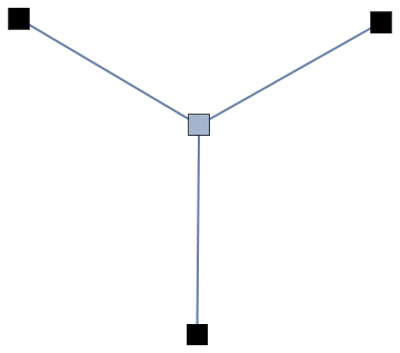
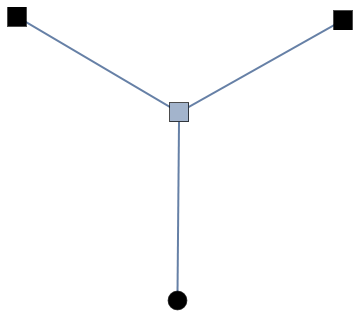
We set up the tree associated with solutions as follows: each solution 𝐱=(x1,x2,x3){\bf x}=(x_{1},x_{2},x_{3}) will be a vertex and neighboring vertices are edge connected if they are obtained from 𝐱{\bf x} by one of the three Vieta maps. As such, we identify coordinates if they are obtained by permutations or double sign changes (noting that Δ\Delta is unchanged under them). By this latter identification, the coordinates are one of two types, namely all positive or exactly one negative. It is then possible to rearrange them into the following canonical forms: (x1,x2,x3)(x_{1},x_{2},x_{3}) or (−x1,x2,x3)(-x_{1},x_{2},x_{3}) with 3≤x1≤x2≤x33\leq x_{1}\leq x_{2}\leq x_{3}. We call the former positive nodes and the latter negative nodes. By Lemma 2.1, for k≥5k\geq 5, every positive node is equivalent to a negative node (or otherwise, by descent is equivalent to the node (3,3,3)(3,3,3) which corresponds to k=0k=0).

We look at the action of the Vieta maps on a positive node. It is clear that x2​x3−2​x1x_{2}x_{3}-2x_{1} and x1​x3−2​x2x_{1}x_{3}-2x_{2} are strictly positive so that Δ1​(𝐱)>Δ​(𝐱)\Delta_{1}({\bf x})>\Delta({\bf x}) and Δ2​(𝐱)>Δ​(𝐱)\Delta_{2}({\bf x})>\Delta({\bf x}). Moreover, the nodes 𝒱1​(𝐱)\mathcal{V}_{1}({\bf x}) and 𝒱2​(𝐱)\mathcal{V}_{2}({\bf x}) are both positive, Next, the argument showing descent in Sec. 2 shows that x1​x2−2​x3≥0x_{1}x_{2}-2x_{3}\geq 0 is impossible so that Δ3​(𝐱)<Δ​(𝐱)\Delta_{3}({\bf x})<\Delta({\bf x}). Here 𝒱3​(𝐱)\mathcal{V}_{3}({\bf x}) may be either positive or negative. We represent these observations by the images Fig.6a and Fig.6b , where square nodes are positive nodes, disc nodes are negative nodes, dark nodes are the Vieta images while the original point is a light node (the vertical ordering of the nodes is determined by the signs of the Δ\Delta-differences from (4.1)).

Next, if we begin with a negative node (so that one replaces x1x_{1} with −x1-x_{1} in the formulae above, it is obvious that Δi​(𝐱)>Δ​(𝐱)\Delta_{i}({\bf x})>\Delta({\bf x}) for all ii and (after a double sign change and reordering) that the 𝒱i​(𝐱)\mathcal{V}_{i}({\bf x}) are all positive. This is represented by Fig. 6c .

It follows now that the tree decomposes into components and each component has a root that is a negative node. Moreover, the negative node occupies the lowest point on the tree, with all other nodes in that component being positive (in other words, Δ\Delta has a minimum on each component and that minimum is determined by a negative node). Thus the negative nodes form a fundamental set, giving us the first case of Theorem 1.1.
Refer to caption
Refer to caption
Refer to caption
Figure 6. Node blocks; top: (a), (b); bottom: (c).

4.2. The case k<0k<0

From Sec. 2 and Lemma 2.2 every lattice point in VkV_{k} is equivalent to one in 𝔖−​(k)\mathfrak{S}^{-}(k). We show that the points in this set are inequivalent. First using (x12−4)​(x22−4)=(2​x3−x1​x2)2−4​(k−4)(x_{1}^{2}-4)(x_{2}^{2}-4)=(2x_{3}-x_{1}x_{2})^{2}-4(k-4) in (4.1) and the similar formulae with the variables permuted, we see that the three terms in square brackets in (4.1) are all positive. Thus the signs of the differences of the Δ\Delta-functions in (4.1) are determined by the three terms x2​x3−2​x1x_{2}x_{3}-2x_{1}, x1​x3−2​x2x_{1}x_{3}-2x_{2} and x1​x2−2​x3x_{1}x_{2}-2x_{3}. The first two are obviously positive, and one sees that the last is non-negative if and only if (x1,x2,x3)∈𝔖−​(k)(x_{1},x_{2},x_{3})\in\mathfrak{S}^{-}(k) Thus, in the tree determined by these points one sees that we have nodes of the type shown in Fig.6(c) with two or three black square vertices emanating from points in 𝔖−​(k)\mathfrak{S}^{-}(k), while for points in the complementary set, we have nodes of the type in Fig.6(a). It follows that the points in 𝔖−​(k)\mathfrak{S}^{-}(k) can serve as the roots of the components of the tree, from which the second case of Theorem 1.1 follows.

4.3. The Cayley surface k=4k=4

Most of the argument above for k≥5k\geq 5 can be applied to the case k=4k=4, and we indicate the necessary modifications. First, we consider solutions of the type (−x1,x2,x3)(-x_{1},x_{2},x_{3}) with x1,x2,x3≥0x_{1},\,x_{2},\,x_{3}\geq 0 satisfying x12+x22+x32+x1​x2​x3=4x_{1}^{2}+x_{2}^{2}+x_{3}^{2}+x_{1}x_{2}x_{3}=4. It is obvious that there are only two solutions up to equivalence, namely (−2,0,0)∼(0,0,2)(-2,0,0)\sim(0,0,2) and (−1,1,1)∼(1,1,2)(-1,1,1)\sim(1,1,2). Hence we need only consider solutions of the type (x1,x2,x3)(x_{1},x_{2},x_{3}) with 0≤x1≤x2≤x30\leq x_{1}\leq\ x_{2}\leq x_{3}. If x1=0x_{1}=0, the only solution is (0,0,2)(0,0,2) while if x1=1x_{1}=1, then the only choice is (1,1,2)(1,1,2). Then by the descent argument in Sec. 2, if x1≥3x_{1}\geq 3, the solution (x1,x2,x3)(x_{1},x_{2},x_{3}) is equivalent to one with one of the coordinates equal to 2. It is trivial that the only solutions of this kind are one of the type (2,a,a)(2,a,a), with a≥0a\geq 0 integers. It suffices now to check the equivalence of these solutions. It is easily checked that the orbits of (2,0,0)(2,0,0), (2,1,1)(2,1,1) and (2,2,2)(2,2,2) contain no other points of the type (2,a,a)(2,a,a) except themselves, so that we assume a≥3a\geq 3.

Following the three formulas in (4.1), if 𝐱=(2,a,a){\bf x}=(2,a,a), then two of the Vieta transformations keep it inert while the third creates a node above it, this new node not being of the same type (we say “above” to mean Δi​(𝐱)>Δ​(𝐱)\Delta_{i}({\bf x})>\Delta({\bf x})). Also following the argument used for k≥5k\geq 5, if 𝐱=(x1,x2,x3){\bf x}=(x_{1},x_{2},x_{3}), with xi≥3x_{i}\geq 3, then two Vieta transformations create nodes above it while a third creates a node below it. It is then easily seen that a tree containing a node of the type (2,a,a)(2,a,a) cannot contain a different node of the same type. Hence we have

Proposition 4.1.

The Cayley surface V4​(ℤ)V_{4}(\mathbb{Z}) has infinitely many inequivalent orbits, each determined by a solution of the type (2,a,a)(2,a,a), with a≥0a\geq 0.

One checks that the (2,0,0)∼(−2,0,0)(2,0,0)\sim(-2,0,0)-component has only 1 element (upto permutation and double sign-change) and so the minimal Δ\Delta-value is Δ⁡(−2,0,0)=9\Delta(-2,0,0)=9. Next, the (2,1,1)(2,1,1)-component has only 2 elements namely (2,1,1)(2,1,1) and (−1,1,1)(-1,1,1). The minimal Δ\Delta-value is Δ⁡(−1,1,1)=−16\Delta(-1,1,1)=-16 while Δ⁡(2,1,1)=5\Delta(2,1,1)=5. Finally, Δ⁡(2,a,a)=9−4​a2<0\Delta(2,a,a)=9-4a^{2}<0 for a≥2a\geq 2. Then the same argument used in Sec. 3.1 can be used to show that any lattice point 𝐱\bf{x} not of these type satisfy Δ⁡(𝐱)≥0\Delta({\bf x})\geq 0, so that the minimal Δ\Delta-value is uniquely determined. Thus, even here each component has a unique minimal Δ\Delta-value, whose point can be used as a generator.

Remark 4.2.

One can use the Δ\Delta-function and the analysis above to deduce a descent procedure. One concludes that either every positive node descends to a negative node or if not, there is an infinite chain of positive nodes on which Δ⁡(𝐱)\Delta({\bf x}) is strictly decreasing. The latter is not possible since Δ⁡(𝐱)≥0\Delta({\bf x})\geq 0 on positive nodes. There are only finitely many negative nodes in 𝔖+​(k)\mathfrak{S}^{+}(k). So we conclude that there are finitely many orbits. Repeating the analysis in the paper also shows that all the negative points are Γ\Gamma-inequivalent and in each orbit Δ\Delta has a minimum value taken at the root of that orbit, so at the only (modulo double sign-changes) negative point on that orbit.

Using Lagrange multipliers on the region on VkV_{k} with xj≥3x_{j}\geq 3 and k→∞k\to\infty, one can show that :

  1. (1)
    min𝐱∈𝔖+​(k)⁡Δ⁡(𝐱)≥k2+18​k32+88​k+6214​k12+O⁡(1);\min_{{\bf x}\in\mathfrak{S}^{+}(k)}\Delta({\bf x})\ \geq\ k^{2}+18k^{\frac{3}{2}}+88k+\frac{621}{4}k^{\frac{1}{2}}+O(1);
  2. (2)
    max𝐱∈𝔖−​(k)⁡Δ⁡(𝐱)≤k2−18​k32+88​k−454​k12+O⁡(1);\max_{{\bf x}\in\mathfrak{S}^{-}(k)}\Delta({\bf x})\ \leq\ k^{2}-18k^{\frac{3}{2}}+88k-\frac{45}{4}k^{\frac{1}{2}}+O(1);
  3. (3)
    min𝐱∈𝔖−​(k)⁡Δ⁡(𝐱)≥−3​k43+O⁡(k).\min_{{\bf x}\in\mathfrak{S}^{-}(k)}\Delta({\bf x})\ \geq\ -3k^{\frac{4}{3}}+O(k).

Hence asymptotically, Δ\Delta behaves like a Minkowski gauge-function, with "successive minima" taken at the root of the orbits; that is if 𝔥⁡(k)\mathfrak{h}(k) is the number of orbits, the first 𝔥⁡(k)\mathfrak{h}(k) minimal values (counted with multiplicity) of Δ\Delta on the lattice points on VkV_{k} occur at the negative points.

5. Parametric solutions on Markoff-type surfaces and Zariski density.

We show in this section that for generic kk, the Markoff surface has no parametric integral points and that the solution set is Zariski dense. We also consider the surfaces given by U1U_{1} and U2U_{2} mentioned in the Introduction.

5.1. Parametric solutions

Lemma 5.1.

For any k∈ℤk\in\mathbb{Z}, let Mk∗M^{*}_{k} be the surface given by M∗​(𝐱)=kM^{*}({\bf x})=k, where

(5.1) M∗​(𝐱)=∑j=13αj​xj+(β1​x2​x3+β2​x1​x3+β3​x1​x2)+x12+x22+ε​x32−x1​x2​x3,M^{*}({\bf x})=\sum_{j=1}^{3}\alpha_{j}x_{j}+\left(\beta_{1}x_{2}x_{3}+\beta_{2}x_{1}x_{3}+\beta_{3}x_{1}x_{2}\right)+x_{1}^{2}+x_{2}^{2}+\varepsilon x_{3}^{2}-x_{1}x_{2}x_{3},

where ε=±1\varepsilon=\pm 1 and αj\alpha_{j}, βj∈ℤ\beta_{j}\in\mathbb{Z} for all jj. Suppose there are polynomials Pj​(t)∈ℤ​[t]P_{j}(t)\in\mathbb{Z}[t] each with non-zero degree, such that M∗​(P1,P2,P3)=kM^{*}(P_{1},P_{2},P_{3})=k identically in tt. Then there are polynomials Q1,Q2∈ℤ⁡[t]Q_{1},Q_{2}\in\mathbb{Z}[t] of non-zero degree and a constant q∈ℤq\in\mathbb{Z} such that M∗​(q,Q1,Q2)=kM^{*}(q,Q_{1},Q_{2})=k identically in tt.

Proof.

Let PjP_{j} have degree dj≠0d_{j}\neq 0 for j=1,2,3j=1,2,3 as above. By comparing degrees in (5.1) we cannot have d1=d2=d3d_{1}=d_{2}=d_{3}, so that there is either a unique djd_{j} exceeding the other two or exactly two of the degrees are the same. The latter does not happen as it implies that at least one of the polynomials is a constant. Hence (comparing degrees in (5.1)) we have that d′′=d′+dd^{\prime\prime}=d^{\prime}+d for some choice of the degrees. It will not matter which subscript represents the largest degree in what follows, so that we put d3=d1+d2d_{3}=d_{1}+d_{2}, with d1d_{1}, d2≥1d_{2}\geq 1.

There is a Vieta affine transformation acting on the surface given by x3↦x4=x1​x2−α3−β1​x2−β2​x1−ε​x3x_{3}\mapsto x_{4}=x_{1}x_{2}-\alpha_{3}-\beta_{1}x_{2}-\beta_{2}x_{1}-\varepsilon x_{3}, so that if P4​(t)P_{4}(t) is the polynomial determined by x4x_{4}, we have

P3​P4=k−P12−P22−β3​P1​P2−α1​P1−α2​P2,P_{3}P_{4}=k-P_{1}^{2}-P_{2}^{2}-\beta_{3}P_{1}P_{2}-\alpha_{1}P_{1}-\alpha_{2}P_{2},

identically in tt. If d4d_{4} is the degree of P4P_{4}, we have d3+d4≤2​max⁡(d1,d2)d_{3}+d_{4}\leq 2\max(d_{1},d_{2}), so that d4≤max⁡(d1,d2)−min⁡(d1,d2)<max⁡(d1,d2)d_{4}\leq\max(d_{1},d_{2})-\min(d_{1},d_{2})<\max(d_{1},d_{2}). Thus we have polynomials P1,P2,P4P_{1},P_{2},P_{4} in place of P1,P2,P3P_{1},P_{2},P_{3} representing integral points on the surface, with the maximal degree reduced by at least one and the new maximum degree is determined by P1P_{1} or P2P_{2}. Either P4P_{4} has degree zero, in which case we are done, or if not, all the new polynomials have non-zero degree. Repeating this descent argument (with a different Vieta transformation) shows that there must be parametric solutions with at least one polynomial constant, and the other two polynomials of non-zero degree. ∎

It is not possible to have parametric solutions to (5.1) with two of the polynomials constant. It follows from the lemma that if parametric solutions exist then there exists q∈ℤq\in\mathbb{Z} and Q1,Q2∈ℤ⁡[t]Q_{1},Q_{2}\in\mathbb{Z}[t] of the same degree dd satisfying (5.1) (it is possible to show that d≤2d\leq 2, if it exists). We now consider some special cases:

  1. (1)

    For the Markoff equation we have Q12+Q22−q​Q1​Q2=k−q2Q_{1}^{2}+Q_{2}^{2}-qQ_{1}Q_{2}=k-q^{2}. Comparing the highest degree term shows that there are integers q1,q2q_{1},q_{2} such that q12+q22−q​q1​q2=0q_{1}^{2}+q_{2}^{2}-qq_{1}q_{2}=0. It follows that q=±2q=\pm 2 and k−4=□k-4=\square. Moreover if k=4+w2k=4+w^{2}, then one has a parametric family of solutions q=2q=2, Q1=tQ_{1}=t and Q2=t+wQ_{2}=t+w. In particular, this means that if kk is generic, there are no parametric solutions to the associated Markoff level set.

  2. (2)

    Consider the Markoff-like surface x12+x22−x32−x1​x2​x3=kx_{1}^{2}+x_{2}^{2}-x_{3}^{2}-x_{1}x_{2}x_{3}=k. If we have parametric solutions as above of the type (Q1,Q2,q)(Q_{1},Q_{2},q), then the argument is identical to the Markoff case so that we conclude there are no such parametric solutions except when k+4=w2k+4=w^{2}, in which case we have the parametric family (t+w,t,2)(t+w,t,2). Next, if either x1x_{1} or x2x_{2} is qq, we have the equation Q12−Q22−q​Q1​Q2=k−q2Q_{1}^{2}-Q_{2}^{2}-qQ_{1}Q_{2}=k-q^{2}, so like the case above, we have q12−q22−q​q1​q2=0q_{1}^{2}-q_{2}^{2}-qq_{1}q_{2}=0. We conclude that q=0q=0 so that when k≠0k\neq 0, Q1Q_{1} and Q2Q_{2} have degree zero, a contradiction. When k=0k=0, we have the parametric family (Q1,0,±Q1)(Q_{1},0,\pm Q_{1}) for any polynomial Q1Q_{1}.

    Remark 5.2.

    This surface has the following features: (i) there are no local obstructions, (ii) for k=4α​k′k=4^{\alpha}k^{\prime} with α≥0\alpha\geq 0 and k′k^{\prime} odd, it has the integral points (0,2α​k′+12,2α​k′−12)(0,2^{\alpha}\frac{k^{\prime}+1}{2},2^{\alpha}\frac{k^{\prime}-1}{2}), (iii) if k′≠1k^{\prime}\neq 1 or α≥3\alpha\geq 3, there are infinitely many integral points, and (iv) there are infinitely many Hasse failures (in particular, k=94k=94 is a Hasse failure). This latter statement follows from an analysis similar to that in Prop. 8.1.

  3. (3)

    Consider the linear deformation U1U_{1} of the Markoff equation considered in (1.9), namely x1+x12+x22+ε​x32−x1​x2​x3=kx_{1}+x_{1}^{2}+x_{2}^{2}+\varepsilon x_{3}^{2}-x_{1}x_{2}x_{3}=k. For any integer kk, and ε=±1\varepsilon=\pm 1, we have the parametric family of integral solutions (−t2+k−4​ε,−t2+t+k−4​ε,2)\left(-t^{2}+k-4\varepsilon,-t^{2}+t+k-4\varepsilon,2\right) .

  4. (4)

    Consider the quadratic deformation U2U_{2} of (1.10): x2​x3−x1​x2+x12+x22+x32−x1​x2​x3=kx_{2}x_{3}-x_{1}x_{2}+x_{1}^{2}+x_{2}^{2}+x_{3}^{2}-x_{1}x_{2}x_{3}=k. For any kk, we have the parametric solutions (−t2+t+k−1,−t2+k−1,1)(-t^{2}+t+k-1,-t^{2}+k-1,1).

5.2. Zariski density

5.2.1.

We prove (1.5) for the Markoff surface for kk not a square (this ensures that if Vk,M​(ℤ)≠∅V_{k,M}(\mathbb{Z})\neq\emptyset, then it has a lattice point with at most one coordinate zero). First note that if 𝐱^=(x^1,x^2,x^3)∈Vk​(ℤ)\hat{{\bf x}}=(\hat{x}_{1},\hat{x}_{2},\hat{x}_{3})\in V_{k}(\mathbb{Z}) and |x^j|≥2|\hat{x}_{j}|\geq 2 for some jj, then |Vk​(ℤ)|=∞|V_{k}(\mathbb{Z})|=\infty. To see this, say |x^1|≥2|\hat{x}_{1}|\geq 2; then the composition of the Vieta transformation 𝒱3\mathcal{V}_{3} with the permutation of x2x_{2} and x3x_{3} yields the transformation (x1,x2,x3)↦(x1,x1​x2−x3,x2)(x_{1},x_{2},x_{3})\mapsto(x_{1},x_{1}x_{2}-x_{3},x_{2}) in Γ\Gamma. This preserves the plane x1=x^1x_{1}=\hat{x}_{1} and VkV_{k}, and it induces the linear action [x^1−11 0]\left[\begin{array}[]{cc}\hat{x}_{1}&-1\\ 1&\ 0\end{array}\right] on this plane. Since |x^1|≥2|\hat{x}_{1}|\geq 2, this element in S​L2​(ℤ)SL_{2}(\mathbb{Z}) is of infinite order, so that its orbit is infinite (since it is not acting on the origin) and its Zariski closure contains the conic section {x1=x^1}∩Vk\{x_{1}=\hat{x}_{1}\}\cap V_{k}. We now argue as in [CZ06]. If Vk​(ℤ)¯\overline{V_{k}(\mathbb{Z})}, the Zariski closure of Vk​(ℤ)V_{k}(\mathbb{Z}) is not VkV_{k}, then it is contained in a finite union of curves in VkV_{k}. Hence there can be at most finitely many x^1\hat{x}_{1}’s with (x^1,x^2,x^3)∈Vk​(ℤ)(\hat{x}_{1},\hat{x}_{2},\hat{x}_{3})\in V_{k}(\mathbb{Z}) with |x^1|≥2|\hat{x}_{1}|\geq 2 (since otherwise Vk​(ℤ)¯\overline{V_{k}(\mathbb{Z})} contains infinitely many distinct conic sections as above). The same applies to x^2\hat{x}_{2} and x^3\hat{x}_{3}, giving |Vk​(ℤ)|<∞|V_{k}(\mathbb{Z})|<\infty. That is we have shown that |Vk​(ℤ)|=∞|V_{k}(\mathbb{Z})|=\infty implies that Vk​(ℤ)¯=Vk\overline{V_{k}(\mathbb{Z})}=V_{k}. To complete the proof of (1.5) note that if |k|>20|k|>20 and (x^1,x^2,x^3)∈Vk​(ℤ)(\hat{x}_{1},\hat{x}_{2},\hat{x}_{3})\in V_{k}(\mathbb{Z}) then for at least one of the jj’s, |x^j|≥2|\hat{x}_{j}|\geq 2 and so |Vk​(ℤ)|≠∅|V_{k}(\mathbb{Z})|\neq\emptyset implies Vk​(ℤ)¯=Vk\overline{V_{k}(\mathbb{Z})}=V_{k}. For the kk’s with |k|≤20|k|\leq 20 we check directly that (1.5) holds. One can show that when k=1, 9, 49k=1,\ 9,\ 49, for example, Vk,M​(ℤ)≠∅V_{k,M}(\mathbb{Z})\neq\emptyset but has only a finite orbit. On the other hand, when k=k12k=k_{1}^{2} with k1k_{1} having an odd prime factor congruent to one modulo 4, then Vk,M​(ℤ)V_{k,M}(\mathbb{Z}) has an infinite orbit, and by the argument above, is Zariski dense.

5.2.2.

We next consider the surface U1U_{1} discussed above and in (1.9). The argument is almost the same as for the Markoff surface except that now we have an affine transformation and a lack of full symmetry in the variables.

As in the case for the Markoff equation, assume that Vk,U1​(ℤ)¯≠Vk,U1\overline{V_{k,U_{1}}(\mathbb{Z})}\neq V_{k,U_{1}} so that it is contained in a finite union of curves. Consider the two Vieta transformations: 𝒱1​(𝐱)=(x2​x3−1−x1,x2,x3)\mathcal{V}_{1}({\bf x})=(x_{2}x_{3}-1-x_{1},x_{2},x_{3}) and 𝒱3​(𝐱)=(x1,x2,x1​x2−x3)\mathcal{V}_{3}({\bf x})=(x_{1},x_{2},x_{1}x_{2}-x_{3}), keeping x2x_{2} fixed. Put 𝐰=(x1,x3)T{\bf w}=(x_{1},x_{3})^{T} so that 𝒱1\mathcal{V}_{1} and 𝒱3\mathcal{V}_{3} act on 𝐰{\bf w}. By abuse of notation, we have

𝒱1​(𝐰)=[−1x20 1]​𝐰+[−10]and𝒱3​(𝐰)=[10−x2−1]​𝐰,\mathcal{V}_{1}({\bf w})=\left[\begin{array}[]{cc}-1&x_{2}\\ 0&\ 1\end{array}\right]{\bf w}+\left[\begin{array}[]{c}-1\\ 0\end{array}\right]\hskip 10.00002pt\text{and}\hskip 10.00002pt\mathcal{V}_{3}({\bf w})=\left[\begin{array}[]{cc}1&0\\ -x_{2}&-1\end{array}\right]{\bf w},

so that we write 𝒱1​𝒱3​(𝐰)=A​𝐰+𝐛\mathcal{V}_{1}\mathcal{V}_{3}({\bf w})=A{\bf w}+{\bf b}, with

A=[−1−x22−x2−x2−1]∈S​L​(2,ℤ),and𝐛=[−10].A=\left[\begin{array}[]{cc}-1-x_{2}^{2}&-x_{2}\\ -x_{2}&\ -1\end{array}\right]\in SL(2,\mathbb{Z}),\hskip 10.00002pt\text{and}\hskip 10.00002pt{\bf b}=\left[\begin{array}[]{c}-1\\ 0\end{array}\right].

Hence (𝒱1​𝒱3)n​𝐰=An​𝐰+∑j=0n−1Aj​𝐛(\mathcal{V}_{1}\mathcal{V}_{3})^{n}{\bf w}=A^{n}{\bf w}+\sum_{j=0}^{n-1}A^{j}{\bf b} for n≥1n\geq 1. If 𝒱1​𝒱3\mathcal{V}_{1}\mathcal{V}_{3} has order nn, it follows that (An−I)​[(A−I)​𝐰+𝐛]=0(A^{n}-I)[(A-I){\bf w}+{\bf b}]=0. Now, if x2≠0x_{2}\neq 0, then AA has infinite order and An−IA^{n}-I is invertible, so that we have (A−I)​𝐰=−𝐛(A-I){\bf w}=-{\bf b}. This is impossible since (A−I)−1​𝐛(A-I)^{-1}{\bf b} is not integral. Hence 𝒱1​𝒱3\mathcal{V}_{1}\mathcal{V}_{3} has infinite order so that the orbit 𝒱1​𝒱3​(x1,x2,x3)\mathcal{V}_{1}\mathcal{V}_{3}(x_{1},x_{2},x_{3}) with x2≠0x_{2}\neq 0 fixed is infinite. The assumption of Zariski density implies that there are only finitely many x2x_{2}’s.

Since the surface given by U1U_{1} is symmetric in x2x_{2} and x3x_{3}, it follows that there are only finitely many x2x_{2} and x3x_{3}’s, from which we conclude that there are at most finitely many lattice points (since x1x_{1} is determined). Starting with the base point 𝐩=(k−4,k−4,2){\bf p}=(k-4,k-4,2) which is on the surface, we see that this is impossible since the orbit 𝒱1​𝒱3​(𝐩)\mathcal{V}_{1}\mathcal{V}_{3}({\bf p}) is infinite if k≠4k\neq 4. Hence Vk,U1​(ℤ)V_{k,U_{1}}(\mathbb{Z}) is Zariski dense in Vk,U1V_{k,U_{1}} for all k≠4k\neq 4. For k=4k=4, we use instead 𝐩=(−1,2,0){\bf p}=(-1,2,0) so that 𝐰≠𝟎{\bf w}\neq{\bf 0}, and the argument above gives an infinite orbit, and Zariski dense.

5.2.3.

The argument for U2U_{2} is almost identical: we use the Vieta transformations 𝒱1​(𝐱)=(x2​x3+x2−x1,x2,x3)\mathcal{V}_{1}({\bf x})=(x_{2}x_{3}+x_{2}-x_{1},x_{2},x_{3}) and 𝒱3​(𝐱)=(x1,x2,x1​x2−x2−x3)\mathcal{V}_{3}({\bf x})=(x_{1},x_{2},x_{1}x_{2}-x_{2}-x_{3}), and have the corresponding matrix equation for 𝒱1​𝒱3​(𝐰)=A​𝐰+𝐛\mathcal{V}_{1}\mathcal{V}_{3}({\bf w})=A{\bf w}+{\bf b}, with

A=[−1+x22−x2x2−1]∈S​L​(2,ℤ),and𝐛=[−x22+x2−x2].A=\left[\begin{array}[]{cc}-1+x_{2}^{2}&-x_{2}\\ x_{2}&\ -1\end{array}\right]\in SL(2,\mathbb{Z}),\hskip 10.00002pt\text{and}\hskip 10.00002pt{\bf b}=\left[\begin{array}[]{c}-x_{2}^{2}+x_{2}\\ -x_{2}\end{array}\right].

The analysis is the same as for U1U_{1} except now we have that An−IA^{n}-I is invertible if |x2|≥3|x_{2}|\geq 3. As above, we derive a contadiction of the finite order assumption since (A−I)−1​𝐛(A-I)^{-1}{\bf b} is not integral. In particular, taking the base point 𝐩=(k−1,k−1,1){\bf p}=(k-1,k-1,1), we conclude that Vk,U2​(ℤ)V_{k,U_{2}}(\mathbb{Z}) is infinite if |k|≥4|k|\geq 4. The reasoning above using the Zariski density assumption shows that there are only finitely many x2x_{2}’s.

Due to the lack of symmetry in the variables, we redo the analysis with x1x_{1} fixed, using 𝒱2​𝒱3​(𝐰)=A​𝐰+𝐛\mathcal{V}_{2}\mathcal{V}_{3}({\bf w})=A{\bf w}+{\bf b}, with 𝒱2​(𝐱)=(x1,x1​x3+x1−x3−x2,x3)\mathcal{V}_{2}({\bf x})=(x_{1},x_{1}x_{3}+x_{1}-x_{3}-x_{2},x_{3}), 𝒱3\mathcal{V}_{3} as before, 𝐰=(x2,x3)T{\bf w}=(x_{2},x_{3})^{T} and

A=[(x1−1)2−11−x1x1−1−1]∈S​L​(2,ℤ),and𝐛=[x10].A=\left[\begin{array}[]{cc}(x_{1}-1)^{2}-1&1-x_{1}\\ x_{1}-1&\ -1\end{array}\right]\in SL(2,\mathbb{Z}),\hskip 10.00002pt\text{and}\hskip 10.00002pt{\bf b}=\left[\begin{array}[]{c}x_{1}\\ 0\end{array}\right].

If |x1−1|≥3|x_{1}-1|\geq 3, we conclude (A−I)​𝐰=−𝐛(A-I){\bf w}=-{\bf b}, and derive a contradiction regarding the finite order assumption. Thus the Zariski density hypothesis implies that there are only finitely many x1x_{1}’s. Hence, again since x3x_{3} is determined by x1x_{1} and x2x_{2}, Vk,U2​(ℤ)V_{k,U_{2}}(\mathbb{Z}) is finite, giving a contradiction. Thus Vk,U2​(ℤ)V_{k,U_{2}}(\mathbb{Z}) is Zariski dense in Vk,U2V_{k,U_{2}} for all |k|≥4|k|\geq 4. For |k|≤4|k|\leq 4, a direct computation gives many eligible candidates for lattice points that lead to Zariski dense.

A much stronger theorem concerning Γ\Gamma invariant holomorphic curves and structures for the surfaces corresponding to (1.8) is proved in ([CL09], Theorem D).

6. Local solutions in ℤp\mathbb{Z}_{p}

Proposition 6.1.

Given k∈ℤk\in\mathbb{Z}, the congruence x12+x22+x32−x1​x2​x3≡k⁡(mod​pn)x_{1}^{2}+x_{2}^{2}+x_{3}^{2}-x_{1}x_{2}x_{3}\equiv k\,({\rm mod}\,p^{n}) has solutions for all primes pp and n≥1n\geq 1 except for the following exceptions : k≡3​(mod​ 4)k\equiv 3\,({\rm mod}\,4), k≡±3​(mod​ 9)k\equiv\pm 3\,({\rm mod}\,9).

We break up the proof into several cases.

It is particularly easy to verify the Proposition for powers of primes p≥5p\geq 5 as follows: recall the Fricke trace identity, namely for any real unimodular matrices AA and BB,

(6.1) 𝔖​(A)2+𝔖​(B)2+𝔖​(A​B)2−𝔖⁡(A)​𝔖​(B)​𝔖​(A​B)=𝔖⁡([A,B])+2,\mathfrak{S}(A)^{2}+\mathfrak{S}(B)^{2}+\mathfrak{S}(AB)^{2}-\mathfrak{S}(A)\mathfrak{S}(B)\mathfrak{S}(AB)=\mathfrak{S}([A,B])+2,

where [A,B]=A​B​A−1​B−1[A,B]=ABA^{-1}B^{-1} is the commutator, and 𝔖⁡()\mathfrak{S}() denotes the trace of the matrix.

Restricting the matrices to S​L​(2,ℤ)SL(2,\mathbb{Z}), one obtains integral solutions to (2.1), with k=t+2k=t+2, where we denote 𝔖⁡([A,B])\mathfrak{S}([A,B]) by tt. We have

Lemma 6.2.

For any prime p≥5p\geq 5, n≥1n\geq 1 and any integer tt, there exists matrices A,B∈S​L​(2,ℤ/pn​ℤ)A,\,B\,\in SL(2,\mathbb{Z}/\penalty p^{n}\mathbb{Z}) such that

𝔖​(A)2+𝔖​(B)2+𝔖​(A​B)2−𝔖⁡(A)​𝔖​(B)​𝔖​(A​B)≡t+2​(mod​pn).\mathfrak{S}(A)^{2}+\mathfrak{S}(B)^{2}+\mathfrak{S}(AB)^{2}-\mathfrak{S}(A)\mathfrak{S}(B)\mathfrak{S}(AB)\equiv t+2\,({\rm mod}\,p^{n})\,.
Proof.

For

A=[abcd],B=[e00f],A,B∈SL(2,ℤ/pnℤ),A=\begin{bmatrix}a&b\\ c&d\end{bmatrix},\hskip 10.00002ptB=\begin{bmatrix}e&0\\ 0&f\end{bmatrix},\hskip 10.00002ptA,B\in SL(2,\mathbb{Z}/\penalty p^{n}\mathbb{Z}),

we have 𝔖⁡([A,B])=2​a​d​e​f−b​c​(e2+f2)≡2−b​c​(e−f)2​(mod​pn)\mathfrak{S}([A,B])=2adef-bc(e^{2}+f^{2})\equiv 2-bc(e-f)^{2}\,({\rm mod}\,p^{n}).

Since p≥5p\geq 5, there exists ee and ff such that (e−f,p)=1(e-f,p)=1 with e​f≡1​(mod​pn)ef\equiv 1\,({\rm mod}\,p^{n}). Then, we choose cc so that c​(e−f)2≡1​(mod​pn)c(e-f)^{2}\equiv 1\,({\rm mod}\,p^{n}). Finally, we choose a=1a=1, b=2−tb=2-t and d=1+b​cd=1+bc.∎∎

Corollary 6.3.

For p≥5p\geq 5 and n≥1n\geq 1, the Markoff congruence x12+x22+x32−x1​x2​x3≡k⁡(mod​pn)x_{1}^{2}+x_{2}^{2}+x_{3}^{2}-x_{1}x_{2}x_{3}\equiv k\,({\rm mod}\,p^{n}) has the solution x1≡2−(k−4)​cx_{1}\equiv 2-(k-4)c, x2≡e+fx_{2}\equiv e+f and x3≡e−f+f​x1x_{3}\equiv e-f+fx_{1}, with e,fe,\,f and cc as in the proof of the Lemma.

The argument above gives the existence of solutions for powers of p≥5p\geq 5. It is useful to have a precise count for the number of solutions modulo pp. For this, it is not any harder to consider the more general problem in

Lemma 6.4.

For p≥3p\geq 3, let NpN_{p} denote the number of solutions to x12+x22+x32−α​x1​x2​x3≡βx_{1}^{2}+x_{2}^{2}+x_{3}^{2}-\alpha x_{1}x_{2}x_{3}\equiv\beta modulo pp. Then

Np={p2+p​(−βp)Lif​p|α,p2+1+(α2​β−4p)L​[3+(βp)L]​potherwise.N_{p}=\left\{\begin{array}[]{ll}p^{2}+p\left(\frac{-\beta}{p}\right)_{\!\!L}&\text{if}\ p|\alpha,\\ \\ p^{2}+1+\left(\frac{\alpha^{2}\beta-4}{p}\right)_{\!\!L}\left[3+\left(\frac{\beta}{p}\right)_{\!\!L}\right]p&\quad\text{otherwise}.\end{array}\right.
Proof.

It is clear we need only consider the cases α=0\alpha=0 and α=1\alpha=1, the latter when p∤αp\nmid\alpha, upon which we multiply through with α2\alpha^{2} and change variables.

Write Sp​(a)=∑uep​(a​u2)S_{p}(a)=\sum_{u}e_{p}(au^{2}) (where ep​(x)=e2​π​i​xpe_{p}(x)=e^{\frac{2\pi ix}{p}}) so that when p∤ap\nmid a, one has Sp​(a)=(ap)L​Sp​(1)S_{p}(a)=\left(\frac{a}{p}\right)_{\!\!L}S_{p}(1). When α=1\alpha=1, putting u≡2​x3−x1​x2​(mod​p)u\equiv 2x_{3}-x_{1}x_{2}\,({\rm mod}\,p) shows that we have the same number of solutions as the congruence

4​(x12+x22)+u2−x12​x22≡4​β​(mod​p),4(x_{1}^{2}+x_{2}^{2})+u^{2}-x_{1}^{2}x_{2}^{2}\equiv 4\beta\,({\rm mod}\,p),

so that

(6.2) Np−p2=1p​∑a≢0Tp​(a)​Sp​(a)​ep​(−4​a​β);N_{p}-p^{2}=\frac{1}{p}\sum_{a\not\equiv 0}T_{p}(a)S_{p}(a)e_{p}(-4a\beta)\,;

here we obtained p2p^{2} solutions when a≡0​(mod​p)a\equiv 0\,({\rm mod}\,p), and we put

Tp​(a)=∑x1,x2ep​(a⁡(4​x12+4​x22−x12​x22))=∑x1ep​(4​a​x12)​Sp​(a⁡(4−x12)).T_{p}(a)=\sum_{x_{1},x_{2}}e_{p}\left(a(4x_{1}^{2}+4x_{2}^{2}-x_{1}^{2}x_{2}^{2})\right)=\sum_{x_{1}}e_{p}(4ax_{1}^{2})S_{p}\left(a(4-x_{1}^{2})\right)\,.

Breaking the sum over x1x_{1} in TpT_{p} above depending on when x1≡±2x_{1}\equiv\pm 2 or not gives us

Tp​(a)=2​p​ep​(16​a)+(ap)L​Sp​(1)​∑x1(4−x12p)L​ep​(4​a​x12).T_{p}(a)=2p\,e_{p}(16a)+\left(\frac{a}{p}\right)_{\!\!L}S_{p}(1)\sum_{x_{1}}\left(\frac{4-x_{1}^{2}}{p}\right)_{\!\!L}e_{p}(4ax_{1}^{2}).

Summing over aa in (6.2) gives Np=p2+E1+E2N_{p}=p^{2}+\mathcalorig{E}_{1}+\mathcalorig{E}_{2}, where

(6.3) E1=2​Sp​(1)​∑a(ap)L​ep​(a⁡(16−4​β))=2​Sp​(1)2​(4−βp)L,\mathcalorig{E}_{1}=2S_{p}(1)\sum_{a}\left(\frac{a}{p}\right)_{\!\!L}\,e_{p}\left(a(16-4\beta)\right)=2S_{p}(1)^{2}\left(\frac{4-\beta}{p}\right)_{\!\!L}\,,

and

(6.4) E2=1p​Sp​(1)2​∑x1(4−x12p)L​∑a≢0ep​(4​a​(x12−β)).\mathcalorig{E}_{2}=\frac{1}{p}S_{p}(1)^{2}\sum_{x_{1}}\left(\frac{4-x_{1}^{2}}{p}\right)_{\!\!L}\ \sum_{a\not\equiv 0}e_{p}\left(4a(x_{1}^{2}-\beta)\right).

Summing over aa in (6.4), we write E2=−E2,1+E2,2\mathcalorig{E}_{2}=-\mathcalorig{E}_{2,1}+\mathcalorig{E}_{2,2} with

E2,1\displaystyle\mathcalorig{E}_{2,1} =Sp​(1)2p​∑x12≢β(4−x12p)L,\displaystyle=\frac{S_{p}(1)^{2}}{p}\sum_{x_{1}^{2}\not{\equiv}\beta}\ \left(\frac{4-x_{1}^{2}}{p}\right)_{\!\!L}\ ,
=Sp​(1)2p​[∑x1(4−x12p)L−(4−βp)L​[1+(βp)L]],\displaystyle=\frac{S_{p}(1)^{2}}{p}\left[\sum_{x_{1}}\ \left(\frac{4-x_{1}^{2}}{p}\right)_{\!\!L}-\left(\frac{4-\beta}{p}\right)_{\!\!L}\left[1+\left(\frac{\beta}{p}\right)_{\!\!L}\right]\right],

and

E2,2=Sp​(1)2p​(p−1)​(4−βp)L​[1+(βp)L].\mathcalorig{E}_{2,2}=\frac{S_{p}(1)^{2}}{p}(p-1)\left(\frac{4-\beta}{p}\right)_{\!\!L}\left[1+\left(\frac{\beta}{p}\right)_{\!\!L}\right].

Since ∑x(4−x12p)L=−(−1p)L\sum_{x}\left(\frac{4-x_{1}^{2}}{p}\right)_{\!\!L}=-\left(\frac{-1}{p}\right)_{\!\!L}, it follows from (6.3) and (6.4) that

Np=p2+2​Sp​(1)2​(4−βp)L+Sp​(1)2p​(−1p)L+Sp​(1)2​(4−βp)L​[1+(βp)L].N_{p}=p^{2}+2S_{p}(1)^{2}\left(\frac{4-\beta}{p}\right)_{\!\!L}+\frac{S_{p}(1)^{2}}{p}\left(\frac{-1}{p}\right)_{\!\!L}+S_{p}(1)^{2}\left(\frac{4-\beta}{p}\right)_{\!\!L}\left[1+\left(\frac{\beta}{p}\right)_{\!\!L}\right].

Using Sp​(1)2=p​(−1p)LS_{p}(1)^{2}=p\left(\frac{-1}{p}\right)_{\!\!L} then gives us

Np=p2+(β−4p)L​[3+(βp)L]​p+1.N_{p}=p^{2}+\left(\frac{\beta-4}{p}\right)_{\!\!L}\left[3+\left(\frac{\beta}{p}\right)_{\!\!L}\right]p+1.

It follows that Np≥p2−4​p+1=(p−2)2−3>0N_{p}\geq p^{2}-4p+1=(p-2)^{2}-3>0 if p≥5p\geq 5. This is also true of p=3p=3 as can be checked with different values of β\beta.

Next, if p|αp|\alpha,

Np−p2=1p​∑a≢0ep​(−β​a)​Sp​(a)3=Sp​(1)3p​∑aep​(−β​a)​(ap)L.N_{p}-p^{2}=\frac{1}{p}\sum_{a\not\equiv 0}e_{p}(-\beta a)S_{p}(a)^{3}=\frac{S_{p}(1)^{3}}{p}\sum_{a}e_{p}(-\beta a)\left(\frac{a}{p}\right)_{\!\!L}.

If p|βp|\beta, then Np=p2N_{p}=p^{2}. If p∤βp\nmid\beta, then the right hand side is p​(−βp)Lp\left(\frac{-\beta}{p}\right)_{\!\!L}.

6.1. Prime powers : p≥5p\geq 5

We have already considered this case in Corollary 6.3, but for completeness we give here the argument using Hensel’s lemma. Let f=x12+x22+x32−x1​x2​x3−kf=x_{1}^{2}+x_{2}^{2}+x_{3}^{2}-x_{1}x_{2}x_{3}-k, considered as three functions of each variable. Then f′f^{\prime} takes the following three forms: 2​x1−x2​x32x_{1}-x_{2}x_{3}, 2​x2−x1​x32x_{2}-x_{1}x_{3} or 2​x3−x1​x22x_{3}-x_{1}x_{2}. To obtain solutions modulo pn+1p^{n+1} from those modulo pnp^{n}, it suffices that at least one of these derivatives not vanish modulo pnp^{n}. We call such triples non-singular. If (x1,x2,x3)(x_{1},x_{2},x_{3}) is such a non-singular solution modulo pnp^{n} with say 2​x1−x2​x3≢0​(mod​pn)2x_{1}-x_{2}x_{3}\not\equiv 0\,({\rm mod}\,p^{n}), then Hensel’s lemma gives a solution to f≡0​(mod​pn+1)f\equiv 0\,({\rm mod}\,p^{n+1}) of the form (y1,x2,x3)(y_{1},x_{2},x_{3}) with y1≡x1​(mod​pn)y_{1}\equiv x_{1}\,({\rm mod}\,p^{n}). This new triple is non-singular modulo pn+1p^{n+1} so that by induction a non-singular solution modulo pp lifts to one modulo pnp^{n} for any n≥1n\geq 1, for any prime p≥5p\geq 5. Note that (3,3,3)(3,3,3) is a non-singular solution when p|kp|k, giving solutions modulo pnp^{n}.

Next suppose the triple (x1,x2,x3)(x_{1},x_{2},x_{3}) is a singular solution of the congruence f≡0​(mod​p)f\equiv 0\,({\rm mod}\,p) for p∤kp\nmid k, so that we have 2​x1≡x2​x32x_{1}\equiv x_{2}x_{3}, 2​x2≡x1​x32x_{2}\equiv x_{1}x_{3} and 2​x3≡x1​x2​(mod​p)2x_{3}\equiv x_{1}x_{2}\,({\rm mod}\,p). If we assume p∤x1​x2​x3p\nmid x_{1}x_{2}x_{3}, then necessarily x12≡x22≡x32x_{1}^{2}\equiv x_{2}^{2}\equiv x_{3}^{2} and x1​x2​x3≡2​x12​(mod​p)x_{1}x_{2}x_{3}\equiv 2x_{1}^{2}\,({\rm mod}\,p). Substituting into f≡0​(mod​p)f\equiv 0\,({\rm mod}\,p) gives x12≡k⁡(mod​p)x_{1}^{2}\equiv k\,({\rm mod}\,p) so that kk must be a non-zero quadratic residue modulo pp, so say k≡u2​(mod​p)k\equiv u^{2}\,({\rm mod}\,p). But then (u,0,0)(u,0,0) is a non-singular solution to f≡0​(mod​p)f\equiv 0\,({\rm mod}\,p), and so by above, lifts to a non-singular solution modulo pnp^{n} for all n≥1n\geq 1.

Finally, suppose p|x1​x2​x3p|x_{1}x_{2}x_{3} with (x1,x2,x3)(x_{1},x_{2},x_{3}) singular. Then pp divides x1x_{1}, x2x_{2} and x3x_{3}, so that p2|kp^{2}|k. But then (3,3,3)(3,3,3) is a non-singular solution modulo p2p^{2} for all p>3p>3. We can now apply Hensel’s lemma as above, starting modulo p2p^{2} and lifting to solutions modulo pnp^{n} for all n≥2n\geq 2 and p>3p>3.

6.2. Prime powers : p=3p=3

The congruence f≡0​(mod​ 3)f\equiv 0\,({\rm mod}\,3) has the following non-singular solutions : when k≡1k\equiv 1, take (1,0,0)(1,0,0); and when k≡−1k\equiv-1, take (0,1,1)(0,1,1). These solutions lift to solutions modulo 3n3^{n} for n≥1n\geq 1.

When k≡0​(mod​ 3)k\equiv 0\,({\rm mod}\,3), the only solution is the singular (0,0,0)(0,0,0). We now consider this case modulo 9. Since 33 divides each of x1x_{1}, x2x_{2} and x3x_{3}, then necessarily when k≡3k\equiv 3 or 66 mod 99, there are no solutions. So assume 9|k9|k, in which case (3,0,0)(3,0,0) is a non-singular solution modulo 9 and so lifts to solutions modulo 3n3^{n}, n≥2n\geq 2.

6.3. Prime powers : p=2p=2

Modulo 2, f′≡f^{\prime}\equiv x1​x2x_{1}x_{2} or x1​x3x_{1}x_{3} or x2​x3x_{2}x_{3}. Thus if kk is even, one may use the non-singular solution (1,1,1)(1,1,1) to obtain solutions modulo powers of 2. When kk is odd, the only solution is the singular (0,0,1)(0,0,1). Then necessarily k≡3​(mod​ 4)k\equiv 3\,({\rm mod}\,4) has no solutions. So assume k≡1​(mod​ 4)k\equiv 1\,({\rm mod}\,4) and we find the non-singular solution (1,0,0)(1,0,0) modulo 4 (note that here one uses f′≡2​x1−x2​x3≢0​(mod​ 4)f^{\prime}\equiv 2x_{1}-x_{2}x_{3}\not\equiv 0\,({\rm mod}\,4)). This then lifts to higher powers of 2.

7. The average of 𝔥M±​(k)\mathfrak{h}_{M}^{\pm}(k): counting lattice points.

We show here that the average of 𝔥M±​(k)\mathfrak{h}_{M}^{\pm}(k) is C±​(log⁡k)2C^{\pm}(\log{k})^{2}, by counting lattice points in the domains given in Theorem 1.1 ((see the paragraph containing (1.6) for definitions). We provide the details for k>5k>5.

Fix u1=au_{1}=a with 3≤a≪K133\leq a\ll K^{\frac{1}{3}} and write u2=mu_{2}=m and u3=nu_{3}=n. We determine the asymptotics of Na​(K)N_{a}(K), the number of pairs (m,n)(m,n) satisfying the inequality a2+m2+n2+a​m​n≤Ka^{2}+m^{2}+n^{2}+amn\leq K with a≤m≤na\leq m\leq n. We have

m≤n≤12​(−a​m+4​(K−a2)+(a2−4)​m2),m\leq n\leq\frac{1}{2}\left(-am+\sqrt{4(K-a^{2})+(a^{2}-4)m^{2}}\right)\,,

so that m≤Kam\leq K_{a}, with Ka=K−a2a+2K_{a}=\sqrt{\frac{K-a^{2}}{a+2}}. Hence

Na​(K)=12​∑a≤m≤Ka{4​(K−a2)+(a2−4)​m2−(a+2)​m}+O⁡(Ka).N_{a}(K)=\frac{1}{2}\sum_{a\leq m\leq K_{a}}\left\{\sqrt{4(K-a^{2})+(a^{2}-4)m^{2}}-(a+2)m\right\}+O\left(\sqrt{\frac{K}{a}}\right)\,.

The function in the sum is decreasing in mm and the contribution from the endpoints are O⁡(K)O(\sqrt{K}). Hence

Na​(K)=12​∫aKa{4​(K−a2)+(a2−4)​x2−(a+2)​x}​𝑑x+O⁡(K).N_{a}(K)=\frac{1}{2}\int_{a}^{K_{a}}\left\{\sqrt{4(K-a^{2})+(a^{2}-4)x^{2}}-(a+2)x\right\}dx+O\left(\sqrt{K}\right)\,.

Changing variables gives

Na​(K)=2​K−a2a2−4​∫αβ{1+x2−a+2a2−4​x}​𝑑x+O⁡(K),N_{a}(K)=2\frac{K-a^{2}}{\sqrt{a^{2}-4}}\int_{\alpha}^{\beta}\left\{\sqrt{1+x^{2}}-\frac{a+2}{\sqrt{a^{2}-4}}x\right\}dx+O\left(\sqrt{K}\right)\,,

where β=a−22\beta=\frac{\sqrt{a-2}}{2} and α=O⁡(a​K−12)\alpha=O(aK^{-\frac{1}{2}}). Replacing α\alpha with zero gives an error of O⁡(K)O(\sqrt{K}) and the integral becomes

12​{β​1+β2+log⁡(β+1+β2)−a+2a2−4​β2}.\frac{1}{2}\left\{\beta\sqrt{1+\beta^{2}}+\log{\left(\beta+\sqrt{1+\beta^{2}}\right)}-\frac{a+2}{\sqrt{a^{2}-4}}\beta^{2}\right\}\,.

Simplifying gives us

Lemma 7.1.

For 3≤a≪K133\leq a\ll K^{\frac{1}{3}}, the number of pairs (m,n)(m,n) satisfying the inequality a2+m2+n2+a​m​n≤Ka^{2}+m^{2}+n^{2}+amn\leq K with a≤m≤na\leq m\leq n is

Na​(K)=log⁡[a−2+a+22]​K−a2a2−4+O⁡(K).N_{a}(K)=\log{\left[\frac{\sqrt{a-2}+\sqrt{a+2}}{2}\right]}\frac{K-a^{2}}{\sqrt{a^{2}-4}}+O(\sqrt{K}).
Lemma 7.2.

Let R+​(K)R^{+}(K) be the number of points (x1,x2,x3)(x_{1},x_{2},x_{3}) satisfying x12+x22+x32+x1​x2​x3≤Kx_{1}^{2}+x_{2}^{2}+x_{3}^{2}+x_{1}x_{2}x_{3}\leq K, with 3≤x1≤x2≤x33\leq x_{1}\leq x_{2}\leq x_{3}  . Then

R+​(K)=136​K​(log⁡K)2+O⁡(K​log⁡K).R^{+}(K)=\frac{1}{36}K(\log{K})^{2}+O(K\log{K})\,.
Proof.

It follows from the previous lemma that

R+​(K)=∑3≤a≤K13log⁡[a−2+a+22]​Ka2−4+O⁡(K56).{}R^{+}(K)=\sum_{{3\leq a\leq K^{\frac{1}{3}}}}\,\log{\left[\frac{\sqrt{a-2}+\sqrt{a+2}}{2}\right]}\frac{K}{\sqrt{a^{2}-4}}+O\left(K^{\frac{5}{6}}\right).

The main term is asymptotic to K2​∑alog⁡aa∼K4​(log⁡K13)2\frac{K}{2}\sum_{a}\frac{\log{a}}{a}\sim\frac{K}{4}(\log{K^{\frac{1}{3}}})^{2}  .∎

We also state, without details, the analogous count for the case of k<0k<0 in Theorem 1.1(ii).

Lemma 7.3.

Let R−​(K)R^{-}(K) be the number of points (x1,x2,x3)(x_{1},x_{2},x_{3}) satisfying x12+x22+x32−x1​x2​x3=−kx_{1}^{2}+x_{2}^{2}+x_{3}^{2}-x_{1}x_{2}x_{3}=-k, with 0<k≤K0<k\leq K and 3≤x1≤x2≤x3≤12​x1​x23\leq x_{1}\leq x_{2}\leq x_{3}\leq\frac{1}{2}x_{1}x_{2} . Then

R−​(K)=148​K​(log⁡K)2+O⁡(K​log⁡K).R^{-}(K)=\frac{1}{48}K(\log{K})^{2}+O(K\log{K})\,.

8. Failures of the Hasse Principle

The fundamental sets allows us to determine Hasse failures for small kk very readily. For example, direct computations reveal that the smallest positive Hasse failure occurs with k=46k=46. That k=46k=46 is a Hasse failure can be verified by applying Theorem 1.1 as follows: either k=46k=46 is exceptional or there exist 3≤x1≤x2≤x33\leq x_{1}\leq x_{2}\leq x_{3} such that x12+x22+x32+x1​x2​x3=46x_{1}^{2}+x_{2}^{2}+x_{3}^{2}+x_{1}x_{2}x_{3}=46. The latter cannot occur since the smallest value of the polynomial is 5454. To determine if 4646 is exceptional, since it is not a sum of two squares and since 42 is not a square, it remains to check if the equation x22+x32−x2​x3=45x_{2}^{2}+x_{3}^{2}-x_{2}x_{3}=45 has any solutions with x2,x3∈ℤx_{2},\ x_{3}\ \in\mathbb{Z}. The equation implies that 3|x23|x_{2} and 3|x33|x_{3}, so that we consider the solvability of y12+y22−y1​y2=5y_{1}^{2}+y_{2}^{2}-y_{1}y_{2}=5. This is equivalent to the solvability of u12+3​u22=20u_{1}^{2}+3u_{2}^{2}=20, which is impossible by congruence modulo 5 or otherwise.

Let Vk​(ℤ)V_{k}(\mathbb{Z}) denote the integral points on the surface x12+x22+x32−x1​x2​x3=kx_{1}^{2}+x_{2}^{2}+x_{3}^{2}-x_{1}x_{2}x_{3}=k, for k∈ℤk\in\mathbb{Z}. For k=4+dk=4+d, the surface VkV_{k} is the singular Cayley surface when reduced modulo dd. Its features, coupled with global quadratic reciprocity, yield failures of strong approximation (mod 4​d4d). For example, assume that n→(4​dn)n\to\left(\frac{4d}{n}\right) is a primitive Dirichlet character (mod 4​d4d) and let Sd⊂ℤ/4​d​ℤS_{d}\subset\mathbb{Z}/4d\mathbb{Z} be the multiplicative closed set {n:(4​dn)=0​or​ 1}\left\{n\ :\ \left(\frac{4d}{n}\right)=0\ \text{or}\ 1\right\}. Then, for any 𝐱=(x1,x2,x3)∈Vk​(ℤ){\bf x}=(x_{1},x_{2},x_{3})\in V_{k}(\mathbb{Z}) one has

(8.1) xj2−4∈Sd(mod 4d),forj=1,2,3.x_{j}^{2}-4\in S_{d}\ (\text{mod}\ 4d)\ ,\ \text{for}\ j=1,2,3\ .

These congruences on xjx_{j} imposed by (8.1) are not consequences of local considerations and so strong approximation fails for Vk​(ℤ)V_{k}(\mathbb{Z}), at least (mod 4​d4d).

To see (8.1), we rewrite (2.1) as

(8.2) w2−4​d=(x12−4)​(x22−4),w^{2}-4d=\left(x_{1}^{2}-4\right)\left(x_{2}^{2}-4\right)\ ,

with w=2​x3−x1​x2w=2x_{3}-x_{1}x_{2}. Now, if x12−4=p1​p2​…​plx_{1}^{2}-4=p_{1}p_{2}\ldots p_{l} with pjp_{j} primes (possibly with repetition), then w2≡4​d​(mod​pj)w^{2}\equiv 4d\ (\text{mod}\ p_{j}) and hence (4​dpj)=0\left(\frac{4d}{p_{j}}\right)=0 or 11. Thus pj∈Sdp_{j}\in S_{d} for each jj, and hence so does x12−4x_{1}^{2}-4. The same applies to x22−4x_{2}^{2}-4 and x32−4x_{3}^{2}-4. Quadratic reciprocity then implies that the xjx_{j}’s must lie in certain congruence classes (mod 4​d4d).

As we now show, by specializing the kk’s and enhancing the analysis above, we can eliminate all the candidate congruence classes and produce families of Hasse failures. We turn to these and the proof of Theorem 1.2(i) in the Introduction, which follows from Prop. 8.1 below.

Proposition 8.1.

For the following choices of kk, Vk​(ℤ)V_{k}(\mathbb{Z}) is empty but Vk​(ℤp)V_{k}(\mathbb{Z}_{p}) is non-empty for all primes pp :

  1. (i).

    For k<0k<0, choose k=4−2​ν2k=4-2\nu^{2}, with odd ν\nu having all its prime factors congruent to 11 or 33 modulo 8.

  2. (ii).

    For k>4k>4, choose k=4+2​ν2k=4+2\nu^{2} with ν\nu having all of its prime factors in the congruence classes {±1}\{\pm 1\} modulo 8, and in addition with ν∈{0,±3,±4}\nu\in\{0,\ \pm 3,\ \pm 4\} modulo 9.

  3. (iii).

    Suppose ℓ≥13\ \ell\geq 13 is a prime number with ℓ≡±4\ell\equiv\pm 4 (mod 9). Then choose k=4+2​ℓ2k=4+2\ell^{2}.

The smallest positive kk here is 342.

Proof.

Writing k=4+2​ϵ​ν2k=4+2\epsilon\nu^{2} with ϵ=±1\epsilon=\pm 1, with odd ν\nu, the congruence conditions ensure that Prop. 6.1 implies Vk​(ℤp)≠∅V_{k}(\mathbb{Z}_{p})\neq\varnothing for all primes pp.

Let (x1,x2,x3)(x_{1},x_{2},x_{3}) be a solution to

(8.3) x12+x22+x32−x1​x2​x3=4+2​ϵ​ν2,x_{1}^{2}+x_{2}^{2}+x_{3}^{2}-x_{1}x_{2}x_{3}=4+2\epsilon\nu^{2}\ ,

with the corresponding

(8.4) w2−8​ϵ​ν2=(x12−4)​(x22−4),w^{2}-8\epsilon\nu^{2}=(x_{1}^{2}-4)(x_{2}^{2}-4)\ ,

with w=2​x3−x1​x2w=2x_{3}-x_{1}x_{2}.

Since ν\nu is odd, 4±2​ν24\pm 2\nu^{2} is not divisible by 4, so that at least one of x1x_{1}, x2x_{2} or x3x_{3} is odd, so say x1x_{1}. Then x12−4≡5≡−3​(mod​ 8)x_{1}^{2}-4\equiv 5\equiv-3\ (\text{mod}\ 8).

Case (i): It follows that x12−4x_{1}^{2}-4 is divisible by a prime number q≡−1​or−3​(mod​ 8)q\equiv-1\ \text{or}\ -3\ (\text{mod}\ 8). Since q∤νq\nmid\nu, it follows from (8.4) that −2-2 is a quadratic residue modulo qq, a contradiction.

Case (ii): It follows that x12−4x_{1}^{2}-4 is divisible by a prime number q≡±5​(mod​ 8)q\equiv\pm 5\ (\text{mod}\ 8). Since q∤νq\nmid\nu, it follows from (8.4) that 22 is a quadratic residue modulo qq, a contradiction.

Case (iii): Recall that for k≥5k\geq 5, if kk is not exceptional, every solution is equivalent to one in the fundamental set 3≤x1≤x2≤x33\leq x_{1}\leq x_{2}\leq x_{3} with x12+x22+x32+x1​x2​x3=k=4+2​ℓ2x_{1}^{2}+x_{2}^{2}+x_{3}^{2}+x_{1}x_{2}x_{3}=k=4+2\ell^{2}. This implies that 3≤x1≤k133\leq x_{1}\leq k^{\frac{1}{3}} and x1≤x2≤(kx1)12x_{1}\leq x_{2}\leq\left(\frac{k}{x_{1}}\right)^{\frac{1}{2}}. Now, the proof above requires that at least one of the variables is odd; but in fact at least 2 variables are odd (by considering the equation modulo 4). It follows that we derive a contradiction if we follow the proof above with q≠ℓq\neq\ell. On the other hand, if q=ℓq=\ell, since two variables are odd, we can choose one, say x1x_{1} satisfying 3≤x1≤k33\leq x_{1}\leq\sqrt{\frac{k}{3}} with ℓ|(x12−4)\ell|(x_{1}^{2}-4). Then ℓ|(x1−2)\ell|(x_{1}-2) or ℓ|(x1+2)\ell|(x_{1}+2) so that x1+2≥ℓ​tx_{1}+2\geq\ell t for some t≥1t\geq 1. Then we get

ℓ−2≤ℓ​t−2≤x1≤4+2​ℓ23,\ell-2\leq\ell t-2\leq x_{1}\leq\sqrt{\frac{4+2\ell^{2}}{3}}\ ,

so that 3​(ℓ−2)2≤4+2​ℓ23(\ell-2)^{2}\leq 4+2\ell^{2}, which implies that ℓ<13\ell<13, a contradiction.

To complete the proof, it remains to check that our choice of kk is not exceptional, that is there are no solutions with say x1x_{1} equal to 00, ±1\pm 1 or ±2\pm 2. If x1=0x_{1}=0, then since two variables are odd, we have x2x_{2} and x3x_{3} are odd with x22+x32=4+2​ℓ2x_{2}^{2}+x_{3}^{2}=4+2\ell^{2}. The left side is congruent to 2 while the right is congruent to 6 modulo 8. Next, if x1=±1x_{1}=\pm 1, we have x22+x32−x2​x3=3+2​ℓ2x_{2}^{2}+x_{3}^{2}-x_{2}x_{3}=3+2\ell^{2}. Completing the square gives us (2​x1−x3)2+3​x32=4​(3+2​ℓ2)(2x_{1}-x_{3})^{2}+3x_{3}^{2}=4(3+2\ell^{2}), so that 8​ℓ28\ell^{2} is a quadratic residue modulo 3. This is a fallacy since 8​ℓ2≡28\ell^{2}\equiv 2. Finally, the case x1=±2x_{1}=\pm 2 is trivially dealt with since it implies that 2 is a square. ∎

We continue below with variants of this construction of Hasse failures, their densities being no more than the kk’s in Prop. 8.1, which is K12​(log⁡K)−12K^{\frac{1}{2}}(\log{K})^{-\frac{1}{2}} and establishes Theorem 1.2(i).

Proposition 8.2.

Suppose ν2≡25​(mod​ 32)\nu^{2}\equiv 25\ (\text{mod}\ 32) with ν\nu having all prime factors ≡±1​(mod​ 12)\equiv\pm 1\ (\text{mod}\ 12). Then, Vk​(ℤ)V_{k}(\mathbb{Z}) is empty with k=4+12​ν2k=4+12\nu^{2}, but has local solutions. The smallest ν\nu is 37, with k=16432k=16432.

Proof.

It is obvious that with the choice of kk, the conditions of Prop. 6.1 are satisfied so that local solutions exist.

We first consider congruences modulo 1212, where the squares are in {0, 1, 4, 9}\{0,\ 1,\ 4,\ 9\}. Suppose (x1,x2,x3)(x_{1},x_{2},x_{3}) is a solution to

(8.5) x12+x22+x32+x1​x2​x3=4+12​ν2,x_{1}^{2}+x_{2}^{2}+x_{3}^{2}+x_{1}x_{2}x_{3}=4+12\nu^{2},

with ν\nu as above.

If 2∤x1​x2​x32\nmid x_{1}x_{2}x_{3}, then x12−4≡5​(mod​ 12)x_{1}^{2}-4\equiv 5\ (\text{mod}\ 12) or is divisible by 3 (the same holding for x2x_{2} and x3x_{3}). From (8.5) we have

(8.6) w2−48​ν2=(x12−4)​(x22−4),w^{2}-48\nu^{2}=(x_{1}^{2}-4)(x_{2}^{2}-4),

so that if x12−4≡5​(mod​ 12)x_{1}^{2}-4\equiv 5\ (\text{mod}\ 12), there is a prime p≡±5​(mod​ 12)p\equiv\pm 5\ (\text{mod}\ 12) with p|(x12−4)p|(x_{1}^{2}-4). This is not possible since p∤νp\nmid\nu implies that 33 is a quadratic residue (mod pp), a fallacy. The same holds for x2x_{2} and x3x_{3}, so that we may assume that x12≡x22≡x32≡1​(mod​ 12)x_{1}^{2}\equiv x_{2}^{2}\equiv x_{3}^{2}\equiv 1\ (\text{mod}\ 12), so that each lies in the set {±1,±5}\{\pm 1,\ \pm 5\} modulo 12. If x1≡±5x_{1}\equiv\pm 5, then in x12−4=(x1−2)​(x2+2)x_{1}^{2}-4=(x_{1}-2)(x_{2}+2), at least one factor is congruent to ±5\pm 5, so that the argument above with a prime pp gives a contradiction. Hence we may assume that x1≡±1​(mod​ 12)x_{1}\equiv\pm 1\ (\text{mod}\ 12), and the same for x2x_{2} and x3x_{3}. But then 9 divides the right hand side of (8.6), a contradiction.

Next, if 2∤x1​x22\nmid x_{1}x_{2}, but 2|x32|x_{3}, we see that a Vieta map gives the solution (x1,x2,−(x1​x2+x3))(x_{1},x_{2},-(x_{1}x_{2}+x_{3})) with all coordinates odd, so that the previous analysis give a contradiction.

Hence we assume x1x_{1}, x2x_{2} and x3x_{3} are all even, so that changing variables gives us the equation

(8.7) y12+y22+y32+2​y1​y2​y3=1+3​ν2,y_{1}^{2}+y_{2}^{2}+y_{3}^{2}+2y_{1}y_{2}y_{3}=1+3\nu^{2},

with the corresponding

(8.8) w12−3​ν2=(y12−1)​(y22−1).w_{1}^{2}-3\nu^{2}=(y_{1}^{2}-1)(y_{2}^{2}-1).

If y1y_{1} is odd, then 8|(y12−1)8|(y_{1}^{2}-1) so that 33 is a quadratic residue mod 8, a fallacy. Hence we assume all y1y_{1}, y2y_{2} and y3y_{3} are even. We now consider congruences modulo 16. We first note that 1+3​ν2≡12​(mod​ 16)1+3\nu^{2}\equiv 12\ (\text{mod}\ 16), so that we cannot have 4 dividing each of the variables.

Next, if 4|y14|y_{1}, 4|y24|y_{2} and y3≡2​(mod​ 4)y_{3}\equiv 2\ (\text{mod}\ 4), then (8.7) gives us y32≡12​(mod​ 16)y_{3}^{2}\equiv 12\ (\text{mod}\ 16), an impossibility. Similarly if 4|y14|y_{1} but y2≡y3≡2​(mod​ 4)y_{2}\equiv y_{3}\equiv 2\ (\text{mod}\ 4), then y22+y32≡12​(mod​ 16)y_{2}^{2}+y_{3}^{2}\equiv 12\ (\text{mod}\ 16), which we see again is impossible. Thus, we may assume that y1≡y2≡y3≡2​(mod​ 4)y_{1}\equiv y_{2}\equiv y_{3}\equiv 2\ (\text{mod}\ 4), in which case we write y1=2​z1y_{1}=2z_{1}, y2=2​z2y_{2}=2z_{2} and y3=2​z3y_{3}=2z_{3}, with 2∤z1​z2​z32\nmid z_{1}z_{2}z_{3}. Then (8.7) becomes

z12+z22+z32+4​z1​z2​z3=1+3​(ν2−14).z_{1}^{2}+z_{2}^{2}+z_{3}^{2}+4z_{1}z_{2}z_{3}=1+3\left(\frac{\nu^{2}-1}{4}\right).

The left hand side is congruent to 7 modulo 8, while the right is congruent to 3. Hence the result follows. ∎

Proposition 8.3.

Suppose ν≡±4​(mod​ 9)\nu\equiv\pm 4\ (\text{mod}\ 9) with ν\nu having all its prime factors congruent to ±1​(mod​ 20)\pm 1\ (\text{mod}\ 20). Then, Vk​(ℤ)V_{k}(\mathbb{Z}) is empty with k=4+20​ν2k=4+20\nu^{2}, but has local solutions. The smallest ν\nu is 41, with k=33624k=33624.

Proof.

The proof is very much the same as the one above, with a small change. The squares modulo 20 lie in the set {0,1,±4,5,9}\{0,1,\pm 4,5,9\} and the odd primes in {±1,±3,±7,±9}\{\pm 1,\pm 3,\pm 7,\pm 9\}.

Write w2−80​ν2=(x12−4)​(x22−4)w^{2}-80\nu^{2}=(x_{1}^{2}-4)(x_{2}^{2}-4). If 5|x15|x_{1}, there must exist a prime p≡±2p\equiv\pm 2 modulo 5 dividing x12−4x_{1}^{2}-4, so that since p∤νp\nmid\nu, 8080 is a quadratic residue modulo pp, which is false using quadratic reciprocity. So we may assume 5∤x1​x2​x35\nmid x_{1}x_{2}x_{3} so that xj2−4x_{j}^{2}-4 is not 11 modulo 2020.

If 2∤x1​x2​x32\nmid x_{1}x_{2}x_{3}, since x1x_{1} is odd, we have x12−4≡−3x_{1}^{2}-4\equiv-3 or 55 modulo 20. Assume the former. Then, if there is a prime factor p|(x12−4)p|(x_{1}^{2}-4), with p≡±3p\equiv\pm 3 or ±7\pm 7 (mod 20), then w2≡80​ν2w^{2}\equiv 80\nu^{2} (mod pp), so that 55 is a quadratic residue modulo pp; that is pp a quadratic residue modulo 5, which is not true. Hence x12−4x_{1}^{2}-4 must have a prime factor p≡9p\equiv 9 (mod 20). But then, x12−4≡3x_{1}^{2}-4\equiv 3 implies that there must be another prime factor q≡±3q\equiv\pm 3 or ±7\pm 7 all modulo 20, and that leads to a contradiction. Hence we cannot have x12−4≡−3x_{1}^{2}-4\equiv-3 (mod 20), and the same being so for x2x_{2} and x3x_{3}. Hence we must have x12−4≡x22−4≡5x_{1}^{2}-4\equiv x_{2}^{2}-4\equiv 5 (mod 20), so that w2−80​ν2=(x12−4)​(x22−4)w^{2}-80\nu^{2}=(x_{1}^{2}-4)(x_{2}^{2}-4) implies that 25|8025|80.

If 2∤x1​x22\nmid x_{1}x_{2}, but 2|x32|x_{3}, the Vieta map gives the solution (x1,x2,−(x1​x2+x3))(x_{1},x_{2},-(x_{1}x_{2}+x_{3})) with all coordinates odd, so that the previous analysis give a contradiction. Hence we assume x1x_{1}, x2x_{2} and x3x_{3} are all even, so that changing variables gives us the equation

(8.9) y12+y22+y32+2​y1​y2​y3=1+5​ν2,y_{1}^{2}+y_{2}^{2}+y_{3}^{2}+2y_{1}y_{2}y_{3}=1+5\nu^{2},

with the corresponding

(8.10) w02−5​ν2=(y12−1)​(y22−1).w_{0}^{2}-5\nu^{2}=(y_{1}^{2}-1)(y_{2}^{2}-1).

If y1y_{1}, y2y_{2} and y3y_{3} are all even, then we have a contradiction in (8.9) since v2≡1v^{2}\equiv 1 (mod 4). If y1y_{1} is odd, then 8|(y12−1)8|(y_{1}^{2}-1) so that 55 is a quadratic residue mod 8, a fallacy. The result follows. ∎

9. Proof of Theorem 1.2(ii)

The proofs for the case k>0k>0 and k<0k<0 are almost identical with the main difference being in the choice of our functions and the domains of the variables. We give here the details for the case k>0k>0 and indicate the modification for k<0k<0 in a remark below.

Let K→∞K\rightarrow\infty be our main (large) parameter, and let AA be a secondary parameter satisfying (logK)2<A≪εKε(\log K)^{2}<A\ll_{\varepsilon}K^{\varepsilon}, with ε>0\varepsilon>0 sufficiently small. Let 𝒜\mathcal{A} be the interval [A,A][\sqrt{A},\ A]. Lastly we use a parameter m=∏p≤LpBm=\prod_{p\leq L}\ p^{B}, where we put L=log⁡Alog⁡log⁡A​Φ​(A)L=\frac{\log{A}}{\log\log{A}}\Phi(A) and B=log⁡log⁡AΦ​(A)2B=\frac{\log\log{A}}{\Phi(A)^{2}} with Φ⁡(A)→∞\Phi(A)\to\infty with AA . Then, m∼A1Φ⁡(A)m\sim A^{\frac{1}{\Phi(A)}} as A→∞A\to\infty.

For any a∈𝒜a\in\mathcal{A}, put

(9.1) ga​(x1,x2)=x12+x22+a​x1​x2andfa​(x1,x1)=ga​(x1,x2)+a2.g_{a}(x_{1},x_{2})=x_{1}^{2}+x_{2}^{2}+ax_{1}x_{2}\hskip 10.00002pt\text{and}\hskip 10.00002ptf_{a}(x_{1},x_{1})=g_{a}(x_{1},x_{2})+a^{2}.

It will be convenient to denote by DaD_{a} the discriminant a2−4a^{2}-4 of the indefinite quadratic form gag_{a} above, for each a∈𝒜a\in\mathcal{A}. Completing the square shows that 4​ga​(x1,x2)=(2​x1+a​x2)2−Da​x224g_{a}(x_{1},x_{2})=(2x_{1}+ax_{2})^{2}-D_{a}x_{2}^{2}, so that we consider the form Gd​(s1,s2)=s12−d​s22G_{d}(s_{1},s_{2})=s_{1}^{2}-ds_{2}^{2} with d=Dad=D_{a} (not a complete square). We then define the sector 𝒮d\mathcal{S}_{d} in the plane as

(9.2) 𝒮d={(s1,s2):s1,s2≥0, 0≤Gd(s1,s2)≤1, 2ds2≤s1≤3ds2},={(x1,x2):x1,x2≥0, 0≤ga​(x1,x2)≤14,12​(2​d−a)​x2≤x1≤12​(3​d−a)​x2}.\begin{split}\mathcal{S}_{d}&=\left\{(s_{1},s_{2})\,:\ s_{1},\ s_{2}\geq 0,\ \ 0\leq G_{d}(s_{1},s_{2})\leq 1,\ \ 2\sqrt{d}s_{2}\leq s_{1}\leq 3\sqrt{d}s_{2}\ \right\}\,,\\ &=\left\{(x_{1},x_{2}):\begin{split}&\quad\quad x_{1},\,x_{2}\geq 0,\ 0\leq g_{a}(x_{1},\,x_{2})\leq\frac{1}{4},\\ &\frac{1}{2}\left(2\sqrt{d}-a\right)x_{2}\leq x_{1}\leq\frac{1}{2}\left(3\sqrt{d}-a\right)x_{2}\end{split}\right\}\,.\end{split}
Remark 9.1.

For k<0k<0 we define ga​(x1,x2)=x12+x22−a​x1​x2g_{a}(x_{1},x_{2})=x_{1}^{2}+x_{2}^{2}-ax_{1}x_{2} and define the sector 𝒮d\mathcal{S}_{d} with the constants 22 and 33 replaced by 13\frac{1}{3} and 12\frac{1}{2} respectively. This then leads to some minor changes for the sector in the variable x1x_{1} and x2x_{2}.∎

Next, we define the scaled region X​𝒮d={(X​s1,X​s2):(s1,s2)∈𝒮a}\sqrt{X}\mathcal{S}_{d}=\left\{\left(\sqrt{X}s_{1},\sqrt{X}s_{2}\right):\ (s_{1},s_{2})\in\mathcal{S}_{a}\right\}. It is easily shown that

Vol​(X​𝒮d)=C​Xd,\text{Vol}(\sqrt{X}\mathcal{S}_{d})=C\frac{X}{\sqrt{d}},

with C=14​log⁡32C=\frac{1}{4}\log{\frac{3}{2}}.

For 2≤k≤K2\leq k\leq K, we define

(9.3) Rd(k)=#{(s1,s2)∈K𝒮d∩ℤ2:Gd(s1,s2)=kand 2|(s1−s2)}.R_{d}(k)=\#\left\{(s_{1},s_{2})\in\sqrt{K}\mathcal{S}_{d}\cap\mathbb{Z}^{2}:\ G_{d}(s_{1},s_{2})=k\ \text{and}\ 2|(s_{1}-s_{2})\ \right\}\,.
Lemma 9.2.

For dd and mm as above we have

∑k≤KRd​(k)=C​K2​d+Oε​(K12+ε).\sum_{k\leq K}\ R_{d}(k)=\ \frac{CK}{2\sqrt{d}}+O_{\varepsilon}\left(K^{\frac{1}{2}+\varepsilon}\right)\,.
Proof.

By the definition of 𝒮d\mathcal{S}_{d}, we break up the sum in s1s_{1} and s2s_{2} into the ranges so that 𝒮d=𝒮d(1)∪𝒮d(2)\mathcal{S}_{d}=\mathcal{S}^{(1)}_{d}\cup\mathcal{S}^{(2)}_{d} with

𝒮d(1)={s2≤K8​d, 2ds2≤s1≤3ds2, 2|(s1−s2)},\mathcal{S}_{d}^{(1)}=\left\{s_{2}\leq\sqrt{\frac{K}{8d}}\ ,\ 2\sqrt{d}s_{2}\leq s_{1}\leq 3\sqrt{d}s_{2},\ 2|(s_{1}-s_{2})\right\}\,,

and

𝒮d(2)={K8​d≤s2≤K3​d, 2ds2≤s1≤K+d​s22, 2|(s1−s2)}.\mathcal{S}_{d}^{(2)}=\left\{\sqrt{\frac{K}{8d}}\leq s_{2}\leq\sqrt{\frac{K}{3d}}\ ,\ 2\sqrt{d}s_{2}\leq s_{1}\leq\sqrt{K+ds_{2}^{2}},\ 2|(s_{1}-s_{2})\,\right\}\,.

The sums are easily evaluated.∎∎

Lemma 9.3.

For aa and mm as above and for any α1\alpha_{1} and α2\alpha_{2}, we have

∑x1≡α1​(m)x2≡α2​(m)fa​(x1,x2)≤K(x1,x2)∈4​K​𝒮Da∩ℤ21=2​C​KDa​m2+Oε​(K34+ε),\sum_{\begin{subarray}{c}x_{1}\equiv\alpha_{1}(m)\\ x_{2}\equiv\alpha_{2}(m)\\ f_{a}(x_{1},x_{2})\leq K\\ (x_{1},x_{2})\in\sqrt{4K}\mathcal{S}_{D_{a}}\cap\mathbb{Z}^{2}\end{subarray}}1=\ \frac{2CK}{\sqrt{D_{a}}m^{2}}+O_{\varepsilon}\left(K^{\frac{3}{4}+\varepsilon}\right),

with the error term uniform is all other variables.

Proof.

By (9.1) we have trivially x1,x2≪Kx_{1},\ x_{2}\ll\sqrt{K} . Assuming 0≤αj<m0\leq\alpha_{j}<m, we put xj=αj+m​ljx_{j}=\alpha_{j}+ml_{j} with 1≤lj≪Km1\leq l_{j}\ll\frac{\sqrt{K}}{m}. Then (x1,x2)∈4​K​𝒮Da∩ℤ2(x_{1},x_{2})\in\sqrt{4K}\mathcal{S}_{D_{a}}\cap\mathbb{Z}^{2} and x2≪K14+εx_{2}\ll K^{\frac{1}{4}+\varepsilon} gives at most O⁡(K12+ε)O(K^{\frac{1}{2}+\varepsilon}) lattice points, so that we may assume that K14+ε≪x1,x2≪KK^{\frac{1}{4}+\varepsilon}\ll x_{1},\ x_{2}\ll\sqrt{K}. It is then easily checked that C1′​l2≤l1≤C2′​l2C_{1}^{\prime}l_{2}\leq l_{1}\leq C_{2}^{\prime}l_{2}, with Cj′=Cj​(1+O⁡(K−14+ε))C_{j}^{\prime}=C_{j}\left(1+O(K^{-\frac{1}{4}+\varepsilon})\right), where we have put C1=12​(2​d−a)C_{1}=\frac{1}{2}\left(2\sqrt{d}-a\right) and C2=12​(3​d−a)C_{2}=\frac{1}{2}\left(3\sqrt{d}-a\right) as in (9.2).

Next

|fa​(x1,x2)−m2​fa​(l1,l2)|≪K12+ε.\big|f_{a}(x_{1},x_{2})-m^{2}f_{a}(l_{1},l_{2})\big|\ll K^{\frac{1}{2}+\varepsilon}.

The error in replacing the condition fa​(x1,x2)≤Kf_{a}(x_{1},x_{2})\leq K with the condition m2​ga​(l1,l2)≤Km^{2}g_{a}(l_{1},l_{2})\leq K is at most O⁡(K12+ε)O(K^{\frac{1}{2}+\varepsilon}) since we are counting lattice points in a hyperbolic segment of width K12+εK^{\frac{1}{2}+\varepsilon}, with the variables restricted as above. Thus

∑x1≡α1​(m)x2≡α2​(m)fa​(x1,x2)≤K(x1,x2)∈4​K​𝒮Da∩ℤ21=∑ga​(l1,l2)≤Km2(l1,l2)∈4​Km2​𝒮Da∗∩ℤ21+Oε​(K12+ε),\sum_{\begin{subarray}{c}x_{1}\equiv\alpha_{1}(m)\\ x_{2}\equiv\alpha_{2}(m)\\ f_{a}(x_{1},x_{2})\leq K\\ (x_{1},x_{2})\in\sqrt{4K}\mathcal{S}_{D_{a}}\cap\mathbb{Z}^{2}\end{subarray}}1\ =\sum_{\begin{subarray}{c}g_{a}(l_{1},l_{2})\leq\frac{K}{m^{2}}\\ (l_{1},l_{2})\in\sqrt{\frac{4K}{m^{2}}}\mathcal{S}^{*}_{D_{a}}\cap\mathbb{Z}^{2}\end{subarray}}1+O_{\varepsilon}\left(K^{\frac{1}{2}+\varepsilon}\right),

where 𝒮∗\mathcal{S}^{*} means the constants have been perturbed by about O⁡(K−14+ε)O(K^{-\frac{1}{4}+\varepsilon}), as discussed above. Completing the square shows that the last sum is over the s1s_{1} and s2s_{2} variables as in (9.2) with the constraint that s1−s2s_{1}-s_{2} is even, and with the constants 22 and 33 defining the inequalities perturbed with the addition of O⁡(K−14+ε)O(K^{-\frac{1}{4}+\varepsilon}). Applying Lemma 9.2 with KK replaced with 4​Km2\frac{4K}{m^{2}} gives the result, with CC replaced with C+O⁡(K−14+ε)C+O(K^{-\frac{1}{4}+\varepsilon}).

∎

Corollary 9.4.

For a∈𝒜a\in\mathcal{A} and k≤Kk\leq K let

ra​(k)=#⁡{(x1,x2)∈4​K​𝒮a∩ℤ2:fa​(x1,x2)=k}.r_{a}(k)=\#\left\{(x_{1},x_{2})\in\sqrt{4K}\mathcal{S}_{a}\cap\mathbb{Z}^{2}:f_{a}(x_{1},x_{2})=k\right\}\,.

Then

∑k≤Kra​(k)=2​C​KDa+Oε​(K12+ε).\sum_{k\leq K}\ r_{a}(k)=\frac{2CK}{\sqrt{D_{a}}}+O_{\varepsilon}\left(K^{\frac{1}{2}+\varepsilon}\right)\,.

We now set

(9.4) b𝒜​(k)=∑a∈𝒜ra​(k),b_{\mathcal{A}}(k)=\sum_{a\in\mathcal{A}}r_{a}(k),

and we are interested in this as a function of kk for 1≤k≤K1\leq k\leq K. From Corollary 9.4, we have

(9.5) ∑1≤k≤Kb𝒜​(k)=C​K​log⁡A+O⁡(K​A−1),\sum_{1\leq k\leq K}b_{\mathcal{A}}(k)=CK\log{A}+O(KA^{-1})\,,

so that the mean-value of b𝒜​(k)b_{\mathcal{A}}(k) is C​log⁡AC\log{A}. Our main goal is to estimate the deviation of b𝒜​(k)b_{\mathcal{A}}(k) from its predicted value in terms of local masses. Let δ⁡(Vk)\delta(V_{k}) denote the formal singular series for

(9.6) Vk:x12+x22+x32+x1​x2​x3=k,V_{k}:\hskip 10.00002pt\hskip 10.00002ptx_{1}^{2}+x_{2}^{2}+x_{3}^{2}+x_{1}x_{2}x_{3}=k,

so that δ⁡(Vk)=∏p<∞δp​(Vk)\delta(V_{k})=\prod_{p<\infty}\delta_{p}(V_{k}), with

δp​(Vk)=limν→∞#​Vk​(ℤ/pν​ℤ)pν.\delta_{p}(V_{k})=\lim_{\nu\to\infty}\frac{\#V_{k}(\mathbb{Z}/p^{\nu}\mathbb{Z})}{p^{\nu}}\,.

These are given explicitly in the Appendices and Section 5. Define

(9.7) δ(m)​(k)=#​Vk​(ℤ/m​ℤ)m2:=rm​(k)m2.\delta^{(m)}(k)=\frac{\#V_{k}(\mathbb{Z}/m\mathbb{Z})}{m^{2}}:=\frac{r_{m}(k)}{m^{2}}\,.

Note that δ(m)​(k)\delta^{(m)}(k) depends on kk modulo mm. With this, we define our variance

(9.8) V⁡(K)=V⁡(K,A,m)=∑k≤K(b𝒜​(k)−C⁡(log⁡A)​δ(m)​(k))2.V(K)=V(K,A,m)=\sum_{k\leq K}\left(b_{\mathcal{A}}(k)-C(\log A)\delta^{(m)}(k)\right)^{2}\,.

We expand (9.8) as Σ1+Σ2+Σ3\Sigma_{1}+\Sigma_{2}+\Sigma_{3}. We have

(9.9) Σ3=C2​(log⁡A)2​∑l⁡(mod​m)δ(m)​(l)2​∑k≤Kk≡l⁡(mod​m)1,=C2​(log⁡A)2​(Km+O⁡(1))​∑l⁡(mod​m)δ(m)​(l)2,=C2​(log⁡A)2​(K+O⁡(m))​δm​(V(2)),\begin{split}\Sigma_{3}&=C^{2}(\log{A})^{2}\sum_{l\,({\rm mod}\,m)}\ \delta^{(m)}(l)^{2}\,\sum_{\begin{subarray}{c}k\leq K\\ k\equiv l({\rm mod}\,m)\end{subarray}}1\,,\\ &=C^{2}(\log{A})^{2}\left(\frac{K}{m}+O(1)\right)\sum_{l\,({\rm mod}\,m)}\delta^{(m)}(l)^{2}\,,\\ &=C^{2}(\log{A})^{2}\left(K+O(m)\right)\delta_{m}\left(V^{(2)}\right)\,,\end{split}

where we define

(9.10) V(2):x12+x22+x32+x1​x2​x3=y12+y22+y32+y1​y2​y3,V^{(2)}:\hskip 10.00002pt\hskip 10.00002ptx_{1}^{2}+x_{2}^{2}+x_{3}^{2}+x_{1}x_{2}x_{3}=y_{1}^{2}+y_{2}^{2}+y_{3}^{2}+y_{1}y_{2}y_{3},

and δm​(V(2))\delta_{m}\left(V^{(2)}\right) is the singular series for V(2)V^{(2)} over ℤ/m​ℤ\mathbb{Z}/m\mathbb{Z}.

Next,

(9.11) Σ2=−2C(logA)∑k≤Kb𝒜(k)δ(m)(k)=−logA∑l⁡(mod​m)δ(m)(l)∑k≤Kk≡l⁡(mod​m)b𝒜(k),=−2ClogA∑l⁡(mod​m)δ(m)(l)∑a∈𝒜∑k≤Kk≡l⁡(mod​m)ra(k).\begin{split}\Sigma_{2}&=-2C(\log{A})\sum_{k\leq K}\,b_{\mathcal{A}}(k)\delta^{(m)}(k)=-\log{A}\sum_{l\,({\rm mod}\,m)}\delta^{(m)}(l)\sum_{\begin{subarray}{c}k\leq K\\ k\equiv l({\rm mod}\,m)\end{subarray}}b_{\mathcal{A}}(k)\,,\\ &=-2C\log{A}\sum_{l\,({\rm mod}\,m)}\delta^{(m)}(l)\sum_{a\in\mathcal{A}}\,\sum_{\begin{subarray}{c}k\leq K\\ k\equiv l({\rm mod}\,m)\end{subarray}}\,r_{a}(k)\,.\end{split}

Now, for each a∈𝒜a\in\mathcal{A}, the last sum in (9.11) above is

(9.12) ∑k≤Kk≡l⁡(mod​m)ra​(k)=∑α1,α2​(mod​m)fa​(α1,α2)≡l⁡(mod​m)∑y1≡α1​(mod​m)y2≡α2​(mod​m)fa​(y1,y2)≤K(y1,y2)∈4​K​𝒮a1.\sum_{\begin{subarray}{c}k\leq K\\ k\equiv l({\rm mod}\,m)\end{subarray}}\,r_{a}(k)=\sum_{\begin{subarray}{c}\alpha_{1},\alpha_{2}({\rm mod}\,m)\\ f_{a}(\alpha_{1},\alpha_{2})\equiv l({\rm mod}\,m)\end{subarray}}\sum_{\begin{subarray}{c}y_{1}\equiv\alpha_{1}\,({\rm mod}\,m)\\ y_{2}\equiv\alpha_{2}\,({\rm mod}\,m)\\ f_{a}(y_{1},y_{2})\leq K\\ (y_{1},y_{2})\in\sqrt{4K}\mathcal{S}_{a}\end{subarray}}1.

Applying Lemma 9.3 to the inner sum gives

∑k≤Kk≡l⁡(mod​m)ra​(k)=∑α1,α2​(mod​m)fa​(α1,α2)≡l⁡(mod​m)2​C​Ka​m2​(1+O⁡(a−2)),\sum_{\begin{subarray}{c}k\leq K\\ k\equiv l\,({\rm mod}\,m)\end{subarray}}\ r_{a}(k)=\sum_{\begin{subarray}{c}\alpha_{1},\alpha_{2}\,({\rm mod}\,m)\\ f_{a}(\alpha_{1},\alpha_{2})\equiv l\,({\rm mod}\,m)\end{subarray}}\frac{2CK}{am^{2}}\left(1+O(a^{-2})\right),

so that

(9.13) ∑k≤Kk≡l⁡(mod​m)b𝒜​(k)=2​C​Km2​∑β⁡(mod​m)α1,α2​(mod​m)fβ​(α1,α2)≡l⁡(mod​m)(∑a∈𝒜a≡β⁡(mod​m)(a−1+O⁡(a−3))),=2​C​Km3​(12​log⁡A+O⁡(A−12))​∑β⁡(mod​m)α1,α2​(mod​m)fβ​(α1,α2)≡l⁡(mod​m)1,=2​C​Km​(12​log⁡A+O⁡(A−12))​δ(m)​(l).\begin{split}\sum_{\begin{subarray}{c}k\leq K\\ k\equiv l\,({\rm mod}\,m)\end{subarray}}\ b_{\mathcal{A}}(k)&=\frac{2CK}{m^{2}}\sum_{\begin{subarray}{c}\beta\,({\rm mod}\,m)\\ \alpha_{1},\alpha_{2}\,({\rm mod}\,m)\\ f_{\beta}(\alpha_{1},\alpha_{2})\equiv l\,({\rm mod}\,m)\end{subarray}}\left(\sum_{\begin{subarray}{c}a\in\mathcal{A}\\ a\equiv\beta\,({\rm mod}\,m)\end{subarray}}\left(a^{-1}+O(a^{-3})\right)\right)\,,\\ &=\frac{2CK}{m^{3}}\left(\frac{1}{2}\log{A}+O(A^{-\frac{1}{2}})\right)\sum_{\begin{subarray}{c}\beta\,({\rm mod}\,m)\\ \alpha_{1},\alpha_{2}\,({\rm mod}\,m)\\ f_{\beta}(\alpha_{1},\alpha_{2})\equiv l\,({\rm mod}\,m)\end{subarray}}1\,,\\ &=\frac{2CK}{m}\left(\frac{1}{2}\log{A}+O(A^{-\frac{1}{2}})\right)\delta^{(m)}(l)\,.\end{split}

Combining (9.11) with (9.13) gives us

(9.14) Σ2=−2C2Km((logA)2+O(A−12logA))∑l⁡(mod​m)δ(m)(l)2,=−2​C2​K​((log⁡A)2+O⁡(A−12​log⁡A))​δm​(V(2)).\begin{split}\Sigma_{2}&=-2C^{2}\frac{K}{m}\left((\log{A})^{2}+O(A^{-\frac{1}{2}}\log{A})\right)\sum_{l\,({\rm mod}\,m)}\delta^{(m)}(l)^{2}\,,\\ &=-2C^{2}K\left((\log{A})^{2}+O(A^{-\frac{1}{2}}\log{A})\right)\delta_{m}(V^{(2)})\,.\end{split}

It remains for us to analyze the difficult case Σ1\Sigma_{1}. We have

(9.15) Σ1=∑k≤Kb𝒜2​(k)=∑a1,a2∈𝒜∑k≤Kra1​(k)​ra2​(k),=∑a∈𝒜∑k≤Kra2​(k)+∑a1,a2∈𝒜a1≠a2∑k≤Kra1​(k)​ra2​(k).\begin{split}\Sigma_{1}=\sum_{k\leq K}b_{\mathcal{A}}^{2}(k)&=\sum_{a_{1},\,a_{2}\in\mathcal{A}}\sum_{k\leq K}r_{a_{1}}(k)r_{a_{2}}(k)\,,\\ &=\sum_{a\in\mathcal{A}}\sum_{k\leq K}r_{a}^{2}(k)+\sum_{\begin{subarray}{c}a_{1},\,a_{2}\in\mathcal{A}\\ a_{1}\neq a_{2}\end{subarray}}\ \sum_{k\leq K}r_{a_{1}}(k)r_{a_{2}}(k)\,.\end{split}

The diagonal term above can be estimated from

Lemma 9.5.
  1. (a).

    For RdR_{d} as in (9.3), we have

    ∑k≤KRd2​(k)≪Kd+K​log⁡Kd​τ​(d),\sum_{k\leq K}R_{d}^{2}(k)\ll\frac{K}{\sqrt{d}}+\frac{K\log{K}}{d}\tau(d)\,,
  2. (b).
    ∑a∈𝒜∑k≤Kra2​(k)≪K​log⁡A.\sum_{a\in\mathcal{A}}\sum_{k\leq K}r_{a}^{2}(k)\ll K\log{A}\,.

where τ⁡()\tau(\ ) is the divisor function, and all implied constants are absolute.

Proof.

Since we are obtaining upper-bounds, we will discard the condition that s1−s2s_{1}-s_{2} is even in the definition of Rd​(k)R_{d}(k). By abuse of notation, we denote this modified counting function by Rd​(k)R_{d}(k) in the proof. Part (b) follows from Part (a) in the same manner that Lemma 9.3 follows from Lemma 9.2, and summing over a∈𝒜a\in\mathcal{A}, giving

∑a∈𝒜∑k≤Kra2​(k)≪K​log⁡A+K​log⁡K​log⁡AA≪K​log⁡A,\sum_{a\in\mathcal{A}}\sum_{k\leq K}r_{a}^{2}(k)\ll K\log{A}+\frac{K\log{K}\log{A}}{\sqrt{A}}\ll K\log{A}\,,

since (log⁡K)2≪A≪Kε(\log{K})^{2}\ll A\ll K^{\varepsilon}.

For the proof of Part (a), we write 𝐬j=(sj,tj){\bf s}_{j}=(s_{j},t_{j}) for j=1,2j=1\,,2 to get

Rd2(k)=#{(𝐬1,𝐬2):s12−dt12=s22−dt22=k,𝐬j∈K𝒮d,j=1, 2},R_{d}^{2}(k)=\#\left\{({\bf s}_{1},{\bf s}_{2})\,:\ s_{1}^{2}-dt_{1}^{2}=s_{2}^{2}-dt_{2}^{2}=k,\ {\bf s}_{j}\in\sqrt{K}\mathcal{S}_{d},\ j=1,\,2\,\right\}\,,

so that we have

(9.16) ∑k≤KRd2(k)=#{(𝐬1,𝐬2):s12−dt12=s22−dt22≤K,𝐬j∈K𝒮d,j=1, 2}.\sum_{k\leq K}R_{d}^{2}(k)=\#\left\{({\bf s}_{1},{\bf s}_{2}):\ s_{1}^{2}-dt_{1}^{2}=s_{2}^{2}-dt_{2}^{2}\leq K,\ {\bf s}_{j}\in\sqrt{K}\mathcal{S}_{d},\ j=1,\,2\,\right\}\,.

Now 𝐬j∈K​𝒮d{\bf s}_{j}\in\sqrt{K}\mathcal{S}_{d} and sj2−d​tj2≤Ks_{j}^{2}-dt_{j}^{2}\leq K imply that

s1,s2≪Kandt1,t2≪Kds_{1}\,,s_{2}\ll\sqrt{K}\hskip 10.00002pt\text{and}\hskip 10.00002ptt_{1}\,,t_{2}\ll\sqrt{\frac{K}{d}}

Switching the roles of t1t_{1} and t2t_{2} in (9.16) shows that

∑k≤KRd2(k)≤#{(𝐬1,𝐬2):s12+dt22=s22+dt12,sj≪K12,tj≪(Kd)12,j=1, 2}.\sum_{k\leq K}R_{d}^{2}(k)\leq\#\left\{({\bf s}_{1},{\bf s}_{2}):\,s_{1}^{2}+dt_{2}^{2}=s_{2}^{2}+dt_{1}^{2},\,s_{j}\ll K^{\frac{1}{2}},t_{j}\ll\left(\frac{K}{d}\right)^{\frac{1}{2}},\ j=1,\,2\,\right\}.

Since the forms are now positive definite, we apply Theorem 2 of [BG06], which gives the estimate in the Lemma.∎∎

The inner sum in the off-diagonal term in (9.15) can be analyzed by using Kloostermann’s method (see [HB96] and [Nie10] for a modern treatment and uniformity with our parameters) to give, for a1≠a2a_{1}\neq a_{2}

(9.17) ∑k≤Kra1​(k)​ra2​(k)=δ∞(K)​(a1,a2)​δfin​(a1,a2)+O⁡(K1−ε0),\sum_{k\leq K}r_{a_{1}}(k)r_{a_{2}}(k)=\delta^{(K)}_{\infty}(a_{1},a_{2})\,\delta_{\textrm{fin}}(a_{1},a_{2})\ +O(K^{1-\varepsilon_{0}})\,,

for some ε0>0\varepsilon_{0}>0.

Here, δ∞(K)​(a1,a2)\delta^{(K)}_{\infty}(a_{1},a_{2}) is the singular integral and δfin​(a1,a2)=∏p<∞δp​(a1,a2)\delta_{\textrm{fin}}(a_{1},a_{2})=\prod_{p<\infty}\delta_{p}(a_{1},a_{2}), where δp​(a1,a2)\delta_{p}(a_{1},a_{2}) is the singular series, both associated to the equation

(9.18) Va1,a2:fa1​(x1,x2)=fa2​(y1,y2),V_{a_{1},a_{2}}:\hskip 10.00002ptf_{a_{1}}(x_{1},x_{2})=f_{a_{2}}(y_{1},y_{2})\,,

with

(9.19) δp​(a1,a2)=limν→∞#​Va1,a2​(ℤ/pν​ℤ)p3​ν.\delta_{p}(a_{1},a_{2})=\lim_{\nu\to\infty}\frac{\#V_{a_{1},a_{2}}\left(\mathbb{Z}/p^{\nu}\mathbb{Z}\right)}{p^{3\nu}}\,.

For the singular integral, let 4​K​𝒮a1,a2=4​K​𝒮a1×4​K​𝒮a2\sqrt{4K}\mathcal{S}_{a_{1},a_{2}}=\sqrt{4K}\mathcal{S}_{a_{1}}\times\sqrt{4K}\mathcal{S}_{a_{2}} and let χa1,a2\chi_{a_{1},a_{2}} be its characteristic function (here we abuse notation by writing 𝒮aj\mathcal{S}_{a_{j}} instead of 𝒮Daj\mathcal{S}_{D_{a_{j}}}). Then,

(9.20) δ∞(K)​(a1,a2)=∫−∞∞[∫ℝ4χa1,a2​(𝐱,𝐲)​e​(t⁡(ga1​(𝐱)−ga2​(𝐲)+a12−a22))​d​𝐱​d​𝐲]​d​t.=limϵ→01ϵ.Vol((𝐱,𝐲)∈4​K𝒮a1,a2:|ga1(𝐱)−ga2(𝐲)+a12−a22|<ϵ),=4​C2​Ka1​a2​[1+O⁡(A−1)].\begin{split}\delta^{(K)}_{\infty}(a_{1},a_{2})&=\int_{-\infty}^{\infty}\left[\int_{\mathbb{R}^{4}}\chi_{a_{1},a_{2}}({\bf x},{\bf y})\,e\left(t(g_{a_{1}}({\bf x})-g_{a_{2}}({\bf y})+a_{1}^{2}-a_{2}^{2})\right)\ \text{d}{\bf x}\text{d}{\bf y}\right]\ \text{d}t\,.\\ &=\lim_{\epsilon\to 0}\frac{1}{\epsilon}.\text{Vol}\left(({\bf x},{\bf y})\in\sqrt{4K}\mathcal{S}_{a_{1},a_{2}}:|g_{a_{1}}({\bf x})-g_{a_{2}}({\bf y})+a_{1}^{2}-a_{2}^{2}|<\epsilon\right)\,,\\ &=\frac{4C^{2}K}{a_{1}a_{2}}\left[1+O(A^{-1})\right]\,.\end{split}

Hence, from (9.15) and (9.17) we have

(9.21) Σ1=4​C2​K​(1+O⁡(A−1))​∑a1,a2∈𝒜a1≠a21a1​a2​δfin​(a1,a2)+O⁡(K​log⁡A+K1−ε0​A2).\Sigma_{1}=4C^{2}K\left(1+O(A^{-1})\right)\sum_{\begin{subarray}{c}a_{1},\,a_{2}\in\mathcal{A}\\ a_{1}\neq a_{2}\end{subarray}}\ \frac{1}{a_{1}a_{2}}\delta_{\textrm{fin}}(a_{1},a_{2})+O\left(K\log{A}+K^{1-\varepsilon_{0}}A^{2}\right)\,.

To analyse the main term in (9.21), we replace δfin​(a1,a2)\delta_{\textrm{fin}}(a_{1},a_{2}) with δ(m)​(a1,a2)\delta^{(m)}(a_{1},a_{2}), where

(9.22) δ(m)​(a1,a2):=#​Va1,a2​(ℤ/m​ℤ)m3.\delta^{(m)}(a_{1},a_{2}):=\frac{\#V_{a_{1},a_{2}}\left(\mathbb{Z}/m\mathbb{Z}\right)}{m^{3}}.

The error term in doing so in (9.21) has size

(9.23) ≪K​∑s≥1∑a1,a2∈𝒜a1≠a2gcd​(Da1,Da2)=s|δfin​(a1,a2)−δ(m)​(a1,a2)|a1​a2.\ll K\sum_{s\geq 1}\sum_{\begin{subarray}{c}a_{1},a_{2}\in\mathcal{A}\\ a_{1}\neq a_{2}\\ \text{gcd}\left(D_{a_{1}},D_{a_{2}}\right)=s\end{subarray}}\ \frac{\big|\delta_{\textrm{fin}}(a_{1},a_{2})-\delta^{(m)}(a_{1},a_{2})\big|}{a_{1}a_{2}}.

By Appendix B, δ(m)​(a1,a2)\delta^{(m)}(a_{1},a_{2}) is suitably close to δfin​(a1,a2)\delta_{\textrm{fin}}(a_{1},a_{2}) unless s=gcd​(Da1,Da2)s=\text{gcd}\left(D_{a_{1}},D_{a_{2}}\right) is in the set

S𝒜,m:={s:s=p1e1…ptetwith eitherej≥Bfor somej,orpj>Lfor somej}.S_{\mathcal{A},m}:=\left\{s:s=p_{1}^{e_{1}}\ldots p_{t}^{e_{t}}\ \text{with either}\ e_{j}\geq B\ \text{for some}\ j,\ \text{or}\ p_{j}>L\ \text{for\ some}\ j\right\}.

Moreover, for such a1a_{1} and a2a_{2}, the difference |δfin​(a1,a2)−δ(m)​(a1,a2)|\big|\delta_{\textrm{fin}}(a_{1},a_{2})-\delta^{(m)}(a_{1},a_{2})\big| is O⁡(τ⁡(s))O\left(\tau(s)\right), with τ(.)\tau(.) the divisor function. Hence the contribution to (9.23) from these is at most

(9.24) ∑s∈S𝒜,mτ⁡(s)​∑a1,a2∈𝒜gcd​(Da1,Da2)=s1a1​a2.\sum_{s\in S_{\mathcal{A},m}}\tau(s)\sum_{\begin{subarray}{c}a_{1},a_{2}\in\mathcal{A}\\ \text{gcd}(D_{a_{1}},D_{a_{2}})=s\end{subarray}}\ \frac{1}{a_{1}a_{2}}.

Since Da≡0D_{a}\equiv 0 (mod kk) occurs only if a≡±2a\equiv\pm 2 (mod s2α\frac{s}{2^{\alpha}}) with 0≤α≤30\leq\alpha\leq 3, the sums in (9.24) above are bounded by

(9.25) (log⁡A)2​∑s∈S𝒜,mτ⁡(s)s2≪(log⁡A)2​min⁡(L,2B)−12,(\log{A})^{2}\sum_{s\in S_{\mathcal{A},m}}\ \frac{\tau(s)}{s^{2}}\ll(\log{A})^{2}\ \min\left(L,2^{B}\right)^{-\frac{1}{2}}\,,

because s∈S𝒜,ms\in S_{\mathcal{A},m} implies s≥min⁡(L,2B)s\geq\min(L,2^{B}) and a1,a2≠±2a_{1},\ a_{2}\neq\pm 2.

Next, for s∉S𝒜,ms\notin S_{\mathcal{A},m}, we write

δfin​(a1,a2)=∏p≤Lδp​(a1,a2)​∏p>Lδp​(a1,a2).\delta_{\textrm{fin}}(a_{1},a_{2})=\prod_{p\leq L}\delta_{p}(a_{1},a_{2})\ \prod_{p>L}\delta_{p}(a_{1},a_{2})\,.

Recall from Prop. B.5 that δp​(a1,a2)=1+O⁡(p−2)\delta_{p}(a_{1},a_{2})=1+O(p^{-2}) if p∤Da1​Da2​(Da1−Da2)p\nmid D_{a_{1}}D_{a_{2}}\left(D_{a_{1}}-D_{a_{2}}\right) when p≥3p\geq 3. We denote these primes by 𝒫(1)\mathcal{P}^{(1)} and include p=2p=2 in this set, and denote the remaining finite set of primes by 𝒫(2)\mathcal{P}^{(2)}. We decompose 𝒫(2)\mathcal{P}^{(2)} further into 𝒫(3)={p≥3:p|gcd(Da1,Da2)}\mathcal{P}^{(3)}=\left\{p\geq 3:p|\text{gcd}\left(D_{a_{1}},D_{a_{2}}\right)\ \right\} and its complement. Then we write

∏p>Lδp​(a1,a2)=∏p∈𝒫(1)p>Lδp​(a1,a2)​∏p∈𝒫(2)p>Lδp​(a1,a2),=∏p∈𝒫(2)p>Lδp​(a1,a2)​(1+O⁡(1L)).\begin{split}\prod_{p>L}\delta_{p}(a_{1},a_{2})&=\prod_{\begin{subarray}{c}p\in\mathcal{P}^{(1)}\\ p>L\end{subarray}}\ \delta_{p}(a_{1},a_{2})\prod_{\begin{subarray}{c}p\in\mathcal{P}^{(2)}\\ p>L\end{subarray}}\delta_{p}(a_{1},a_{2})\,,\\ &=\prod_{\begin{subarray}{c}p\in\mathcal{P}^{(2)}\\ p>L\end{subarray}}\delta_{p}(a_{1},a_{2})\,\left(1+O\left(\frac{1}{L}\right)\right)\,.\end{split}

Since s∉S𝒜,ms\notin S_{\mathcal{A},m}, if p>Lp>L we have (using Prop. B.5 again)

log∏p∈𝒫(2)p>Lδp(a1,a2)=∑p∈𝒫(2)p>Lcpp+O(1L),\log{\prod_{\begin{subarray}{c}p\in\mathcal{P}^{(2)}\\ p>L\end{subarray}}\delta_{p}(a_{1},a_{2})}=\sum_{\begin{subarray}{c}p\in\mathcal{P}^{(2)}\\ p>L\end{subarray}}\frac{c_{p}}{p}+\ O\left(\frac{1}{L}\right)\,,

with coefficients cpc_{p} satisfying |cp|≤1|c_{p}|\leq 1. Since a1≠±a2a_{1}\neq\pm a_{2} and aj≠±2a_{j}\neq\pm 2, the set 𝒫(2)\mathcal{P}^{(2)} has the bound card​(𝒫(2))≪log⁡Alog⁡log⁡A\text{card}(\mathcal{P}^{(2)})\ll\frac{\log{A}}{\log\log{A}}, as it contains those primes dividing Da1D_{a_{1}} or Da2D_{a_{2}} or (Da1−Da2)\left(D_{a_{1}}-D_{a_{2}}\right). Hence the sum over 𝒫(2)\mathcal{P}^{(2)} above is bounded by log⁡AL​log⁡log​A≪Φ​(A)−1\frac{\log{A}}{L\log\log{A}}\ll\Phi(A)^{-1}. Thus, for s∉S𝒜,ms\notin S_{\mathcal{A},m} we have

δfin​(a1,a2)=∏p≤Lδp​(a1,a2)×(1+O⁡(1Φ⁡(A))).\delta_{\textrm{fin}}(a_{1},a_{2})=\prod_{p\leq L}\delta_{p}(a_{1},a_{2})\times\left(1+O\left(\frac{1}{\Phi(A)}\right)\right)\,.

To analyse this further, we write δ(mCLOSE​(a1,a2)=∏p≤Lδp(m)​(a1,a2)\delta^{(m}(a_{1},a_{2})=\prod_{p\leq L}\ \delta^{(m)}_{p}(a_{1},a_{2}). Then one has

(9.26) δp​(a1,a2)=1+∑l=1∞Nl​(a1,a2)andδp(m)​(a1,a2)=1+∑l=1BNl​(a1,a2),\delta_{p}(a_{1},a_{2})=1+\sum_{l=1}^{\infty}N_{l}(a_{1},a_{2})\hskip 10.00002pt\text{and}\hskip 10.00002pt\delta^{(m)}_{p}(a_{1},a_{2})=1+\sum_{l=1}^{B}N_{l}(a_{1},a_{2}),

where

(9.27) Nl​(a1,a2)=p−4​l​∑∗b⁡(mod​pl)∗​∑𝐱,𝐲⁡(mod​pl)e⁡(ga1​(𝐱)−ga2​(𝐲)+Da1−Da2pl​b).N_{l}(a_{1},a_{2})=p^{-4l}\sideset{}{{}^{*}}{\sum}_{b\,({\rm mod}\,p^{l})}\,\sum_{{\bf x},\,{\bf y}\,({\rm mod}\,p^{l})}\ e\left(\frac{g_{a_{1}}({\bf x})-g_{a_{2}}({\bf y})+D_{a_{1}}-D_{a_{2}}}{p^{l}}b\right)\,.

Then for s∉S𝒜,ms\notin S_{\mathcal{A},m}, one has by Prop B.4 that δp​(a1,a2)=δp(m)​(a1,a2)+O⁡(p−B)\delta_{p}(a_{1},a_{2})=\delta^{(m)}_{p}(a_{1},a_{2})+O(p^{-B}). It follows that the contribution to (9.23) is

K∑s≥1s∉S𝒜,m∑a1,a2∈𝒜a1≠a2gcd​(Da1,Da2)=s|δfin​(a1,a2)−δ(m)​(a1,a2)|a1​a2≪K​min⁡(Φ⁡(A),2B)−1​∑a1,a2∈𝒜a1≠a2|δ(m)​(a1,a2)|a1​a2,≪K​min⁡(Φ⁡(A),2B)−1​(log⁡A)2,\begin{split}K\sum_{\begin{subarray}{c}s\geq 1\\ s\notin S_{\mathcal{A},m}\end{subarray}}\sum_{\begin{subarray}{c}a_{1},\ a_{2}\in\mathcal{A}\\ a_{1}\neq a_{2}\\ \text{gcd}\left(D_{a_{1}},D_{a_{2}}\right)=s\end{subarray}}&\frac{\big|\delta_{\textrm{fin}}(a_{1},a_{2})-\delta^{(m)}(a_{1},a_{2})\big|}{a_{1}a_{2}}\\ &\ll K\min\left(\Phi(A),2^{B}\right)^{-1}\sum_{\begin{subarray}{c}a_{1},\ a_{2}\in\mathcal{A}\\ a_{1}\neq a_{2}\end{subarray}}\ \frac{\big|\delta^{(m)}(a_{1},a_{2})\big|}{a_{1}a_{2}},\\ &\ll K\min\left(\Phi(A),2^{B}\right)^{-1}(\log{A})^{2}\,,\end{split}

using δ(m)​(a1,a2)≪τ⁡(gcd​(a1,a2))\delta^{(m)}(a_{1},a_{2})\ll\tau(\text{gcd}(a_{1},a_{2})).

We choose Φ⁡(A)=12​log⁡log⁡Alog⁡log⁡log⁡A\Phi(A)=\frac{1}{2}\sqrt{\frac{\log\log A}{\log\log\log A}} so that Φ​(A)2≪2B=o⁡(L)\Phi(A)^{2}\ll 2^{B}=o(L). Substituting into (9.21) gives us

(9.28) Σ1=4​C2​K​∑a1,a2∈𝒜a1≠a2δ(m)​(a1,a2)a1​a2+O⁡(K​Φ​(A)−1​(log⁡A)2).\Sigma_{1}=4C^{2}K\sum_{\begin{subarray}{c}a_{1},\ a_{2}\in\mathcal{A}\\ a_{1}\neq a_{2}\end{subarray}}\ \frac{\delta^{(m)}(a_{1},a_{2})}{a_{1}a_{2}}+O\left(K\Phi(A)^{-1}(\log{A})^{2}\right)\,.

Since δ(m)​(a1,a2)\delta^{(m)}(a_{1},a_{2}) is periodic modulo mm, the sum in (9.28) can be analyzed as in (9.9), giving

(9.29) Σ1=4​C2​K​∑α1​(mod​m)α2​(mod​m)δ(m)​(α1,α2)​(12​log⁡A)2m2+O⁡(K​Φ​(A)−1​(log⁡A)2),=C2​K​(log⁡A)2​δm​(V(2))+O⁡(K​Φ​(A)−1​(log⁡A)2).\begin{split}\Sigma_{1}&=4C^{2}K\sum_{\begin{subarray}{c}\alpha_{1}\,({\rm mod}\,m)\\ \alpha_{2}\,({\rm mod}\,m)\end{subarray}}\,\delta^{(m)}(\alpha_{1},\alpha_{2})\frac{\left(\frac{1}{2}\log{A}\right)^{2}}{m^{2}}+O\left(K\Phi(A)^{-1}\left(\log{A}\right)^{2}\right),\\ &=C^{2}K\left(\log{A}\right)^{2}\delta_{m}\left(V^{(2)}\right)+O\left(K\Phi(A)^{-1}\left(\log{A}\right)^{2}\right)\,.\end{split}

Combining (9.9), (9.14) and (9.28) into (9.8) gives us the key cancellation and hence the estimate on the variance V⁡(K)V(K).

Proposition 9.6.

Let K→∞K\rightarrow\infty, let 𝒜\mathcal{A} be the interval [A,A][\sqrt{A},\ A] with AA satisfying (logK)2<A≪εKε(\log K)^{2}<A\ll_{\varepsilon}K^{\varepsilon}, with ε>0\varepsilon>0 sufficiently small. Then with Φ⁡(A)=12​log⁡log⁡Alog⁡log⁡log⁡A\Phi(A)=\frac{1}{2}\sqrt{\frac{\log\log A}{\log\log\log A}}, we have

∑k≤K[b𝒜​(k)−C⁡(log⁡A)​δ(m)​(k)]2≪K​Φ​(A)−1​(log⁡A)2.\sum_{k\leq K}\left[b_{\mathcal{A}}(k)-C(\log A)\delta^{(m)}(k)\right]^{2}\ll K\Phi(A)^{-1}\left(\log{A}\right)^{2}\ .
Remark 9.7.

One can remove the auxiliary parameter BB in the Proposition above with

δ(m)​(k)=∏p≤Lδp​(k)+O⁡(2−B),\delta^{(m)}(k)=\prod_{p\leq L}\delta_{p}(k)+O(2^{-B}),

as follows. From (B.2) and (9.6), we have δ⁡(Vk)=∏p<∞δp​(k)\delta(V_{k})=\prod_{p<\infty}\delta_{p}(k) with δp​(k)=1+∑l≥1Nl​(k)\delta_{p}(k)=1+\sum_{l\geq 1}N_{l}(k), where Nl​(k)N_{l}(k) is given in (B.1) and are all evaluated in the Appendix . Similarly, one can show that δ(m)​(k)=∏p≤Lδp(m)​(k)\delta^{(m)}(k)=\prod_{p\leq L}\delta^{(m)}_{p}(k) with δp(m)​(k)=1+∑1≤l≤BNl​(k)\delta^{(m)}_{p}(k)=1+\sum_{1\leq l\leq B}N_{l}(k) . Then, it follows from Prop. B.1 that δp(m)​(k)=δp​(k)+O⁡(p−B)\delta^{(m)}_{p}(k)=\delta_{p}(k)+O(p^{-B}). Applying Prop B.2 then gives the result. ∎

9.1. Lower bound for δ(m)​(k)\delta^{(m)}(k) for most admissible kk’s

To complete the proof of Theorem 1.2(ii), we need to estimate, for ε>0\varepsilon>0

(9.30) |{0≤k≤K:kadmissible,δ(m)(k)<ε}|.\big|\big\{0\leq k\leq K\,:\,k\ \text{admissible},\ \delta^{(m)}(k)<\varepsilon\big\}\big|\,.

By Props. B.5 and B.12 in the Appendix, and Remark 9.7 , we can write

(9.31) δ(m)​(k)=∏p≤L(1+N1,p​(k)+Cp​(k))+o⁡(1),\delta^{(m)}(k)=\prod_{p\leq L}\left(1+N_{1,p}(k)+\mathcalorig{C}_{p}(k)\right)+o(1),

where we indicate the dependence of pp in the definition of NlN_{l}, and with Cp​(k)\mathcalorig{C}_{p}(k) coming from the Nl,pN_{l,p}’s with l≥2l\geq 2. Since we are assuming that kk is admissible, we can ignore the primes p=2p=2 and p=3p=3 since then these local factors are bounded from below. For p≥5p\geq 5, the problematic case of Cp​(k)\mathcalorig{C}_{p}(k) in (9.31) is, by Prop. B.1, of the form 4β​p−1+O⁡(p−2)4^{\beta}p^{-1}+O\left(p^{-2}\right). So, up to O⁡(p−2)O\left(p^{-2}\right), which can be ignored for our purposes of bounding δ(m)​(k)\delta^{(m)}(k) from below, we have that

(9.32) δ(m)​(k)≫∏p≤L(1+N1,p​(k)+O⁡(1p2))+o⁡(1),≫∏p≤L(1+χ​(k−4)​(3+χ​(k))p),\displaystyle\begin{split}\delta^{(m)}(k)&\gg\prod_{p\leq L}\left(1+N_{1,p}(k)+O\left(\frac{1}{p^{2}}\right)\right)+o(1)\,,\\ &\gg\prod_{p\leq L}\left(1+\frac{\chi(k-4)\left(3+\chi(k)\right)}{p}\right)\,,\end{split}

where χ\chi is the Legendre symbol modulo pp. Hence

(9.33) [δ(m)​(k)]−1≪∏p≤L(1−χ​(k−4)​(3+χ​(k))p),=∑n≤Mμ⁡(n)​A​(k,n)n,\displaystyle\begin{split}\left[\delta^{(m)}(k)\right]^{-1}&\ll\prod_{p\leq L}\left(1-\frac{\chi(k-4)\left(3+\chi(k)\right)}{p}\right),\\ &=\sum_{n\leq M}\ \frac{\mu(n)A(k,n)}{n}\,,\end{split}

where A⁡(k,n)=A⁡(k,p1)​…​A​(k,pl)A(k,n)=A(k,p_{1})\ldots A(k,p_{l}) if n=p1​…​pln=p_{1}\ldots p_{l} , M=(∏p≤Lp)≤m≪KεM=\left(\prod_{p\leq L}p\right)\leq m\ll K^{\varepsilon}, and

(9.34) A⁡(k,p)={χ​(k−4)​(3+χ​(k))ifp≥5,0otherwise.A(k,p)=\left\{\begin{array}[]{ll}\chi(k-4)\left(3+\chi(k)\right)&\text{if}\ \ p\geq 5\,,\\ \quad\quad 0&\text{otherwise}\ .\end{array}\right.

Since A⁡(k,n)A(k,n) as a function of kk is periodic of period nn, we have

(9.35) ∑k≤KA⁡(k,n)=Kn​∑k⁡(mod​n)A⁡(k,n)+O⁡(n).\sum_{k\leq K}A(k,n)=\frac{K}{n}\sum_{k\,({\rm mod}\,n)}A(k,n)+O(n)\,.

By multiplicativity, the completed sum

∑k⁡(mod​n)A⁡(k,n)=∏p|n(∑k⁡(mod​p)A⁡(k,p))=μ⁡(n),\sum_{k\,({\rm mod}\,n)}A(k,n)=\prod_{p|n}\left(\sum_{k\,({\rm mod}\,p)}A(k,p)\right)=\mu(n),

since ∑k⁡(mod​p)χ⁡(k−4)=0\sum_{k\,({\rm mod}\,p)}\chi(k-4)=0 and ∑k⁡(mod​p)χ⁡(k−4)​χ​(k)=−1\sum_{k\,({\rm mod}\,p)}\chi(k-4)\chi(k)=-1. Hence

∑k≤KA⁡(k,n)=μ⁡(n)n​K+O⁡(n),\sum_{k\leq K}A(k,n)=\frac{\mu(n)}{n}K+O(n),

so that by (9.33) we have

∑k≤Kk​admissible[δ(m)​(k)]−1≪K⁡(∑n1n2)+M≪K.\sum_{\begin{subarray}{c}k\leq K\\ k\,\text{admissible}\end{subarray}}\left[\delta^{(m)}(k)\right]^{-1}\ll K\left(\sum_{n}\frac{1}{n^{2}}\right)+M\ll K.

Hence, it follows that for any ε>0\varepsilon>0

(9.36) |{0≤k≤K:kadmissible,δ(m)(k)<ε}|≪εK.\big|\big\{0\leq k\leq K:\ k\ \text{admissible}\,,\ \delta^{(m)}(k)<\varepsilon\big\}\big|\ll\varepsilon K.

Finally, combining (9.36) with the variance estimate in Prop. 9.6 gives Theorem 1.2(ii).∎

10. Computations

We computed all the Hasse failures (HF) for positive k≤Kk\leq K with KK about 564 million and present some data associated with this.

By definition there are no HF’s in the congruence classes 33 (mod 4) and ±3\pm 3 (mod 9). We tabulate in Table 1 the percentages in some other congruence classes: more precisely this is the quantity λ=100×#⁡{ HF’s in a congruence class}/#⁡{ HF’s }\lambda=100\times\#\{\text{ HF's in a congruence class}\}/\#\{\text{ HF's }\}.

Class (mod 4) λ%\lambda\%
0 30.6733
1 28.1317
2 41.195
Class (mod 3) λ%\lambda\%
0 42.2078
1 43.2872
2 14.5051
Class (mod 9) λ%\lambda\%
0 42.2078
1 19.023
4 4.462
7 19.802
Class (mod 9) λ%\lambda\%
2 4.831
5 4.833
8 4.841
Table 1. Percentages of Hasse failures in congruence classes.

The number of admissible kk’s (see Sec. 3) in the interval [1,K][1,K] we denote by A⁡(K)\mathcalorig{A}(K), and is asymptotically 712​K\frac{7}{12}K. The admissibles consist of the exceptional kk’s, of which there are O⁡(Klog⁡K)O(\frac{K}{\sqrt{\log{K}}}) members, the generic kk’s consisting of the HF’s and the generic kk’s with 𝔥⁡(k)>0\mathfrak{h}(k)>0. For K≥5K\geq 5, let AH​F​(K)\mathcalorig{A}_{\scriptscriptstyle HF}(K) denote the number of HF’s in the interval [5,K][5,K]. By the arguments in Sec. 7, we know that AH​F​(K)→∞\mathcalorig{A}_{\scriptscriptstyle HF}(K)\rightarrow\infty with KK, and more precisely AH​F(K)≫ϵK12−ϵ\mathcalorig{A}_{\scriptscriptstyle HF}(K)\gg_{\epsilon}K^{\frac{1}{2}-\epsilon} for any ϵ>0\epsilon>0. While we do not know the exact order of AH​F​(K)\mathcalorig{A}_{\scriptscriptstyle HF}(K), Theorem 1.2(ii) shows that it is o⁡(K)o(K), and we consider this question here computationally, for which we compare AH​F​(K)\mathcalorig{A}_{\scriptscriptstyle HF}(K) with A⁡(K)\mathcalorig{A}(K). There are two possible models to consider, namely (1) AH​F​(K)∼A​(K)θ\mathcalorig{A}_{\scriptscriptstyle HF}(K)\sim\mathcalorig{A}(K)^{\theta} for some 0<θ<10<\theta<1 or (2) AH​F​(K)∼A⁡(K)/log⁡A​(K)θ\mathcalorig{A}_{\scriptscriptstyle HF}(K)\sim\mathcalorig{A}(K)/\log{\mathcalorig{A}(K)}^{\theta}. To check these cases, we compute log⁡AH​F​(K)/log⁡A⁡(K)\log{\mathcalorig{A}_{\scriptscriptstyle HF}(K)}/\log{\mathcalorig{A}(K)} with A⁡(K)=712​K\mathcalorig{A}(K)=\frac{7}{12}K.

For K∼564×106K\sim 564\times 10^{6} put L=log⁡KL=\log K, and let

(10.1) f⁡(K)=0.887516−8.06653​L−2−21.8923​L−3+2.38097​L−4+3.35656​L−5.f(K)=0.887516\,-8.06653\ L^{-2}-21.8923\ L^{-3}+2.38097\ L^{-4}+3.35656\ L^{-5}.

Using f⁡(K)f(K) as a predictor for log⁡AH​F​(K)log⁡A⁡(K)\frac{\log{\mathcalorig{A}_{\scriptscriptstyle HF}(K)}}{\log{\mathcalorig{A}(K)}} we compare AH​F​(K)\mathcalorig{A}_{\scriptscriptstyle HF}(K) with P⁡(K)\mathcalorig{P}(K), the integer part of A​(K)f⁡(K)\mathcalorig{A}(K)^{f(K)} and tabulate also the relative percentage error E⁡(K)=100×AH​F​(K)−P​(K)P⁡(K)\mathcalorig{E}(K)=100\times\frac{\mathcalorig{A}_{\scriptscriptstyle HF}(K)-\mathcalorig{P}(K)}{\mathcalorig{P}(K)}, in Table 4, page 4. The KK’s given are each a multiple of 100,800 but otherwise is a sample. The data was gathered by subdividing the interval [1,K][1,K] into subintervals of length 100,800 and computing AH​F​(K)\mathcalorig{A}_{\scriptscriptstyle HF}(K) at the endpoints.

We first show, in Fig. 7, the graph of the “percentages of the Hasse failures”, namely the quantity 100×AH​F​(K)A⁡(K)100\times\frac{\mathcalorig{A}_{\scriptscriptstyle HF}(K)}{\mathcalorig{A}(K)}, together with the prediction P⁡(K)\mathcalorig{P}(K). There were a total of 23,298,27723,298,277 HF’s (with K=564,062,446K=564,062,446) but we plot 5,5955,595 sample points. Next, Fig. 8 is a plot of log⁡AH​F​(K)log⁡A⁡(K)\frac{\log{\mathcalorig{A}_{\scriptscriptstyle HF}(K)}}{\log{\mathcalorig{A}(K)}} together with the approximation f⁡(K)f(K) in (10.1). In both graphs, the approximation curves and data points are too close to show up as separate curves, and so we plot only the data points. We also indicate in Table 2, the quality of the approximations in Fig. 9 and Fig. 10.

Figure 7. Percentages of Hasse failures: 100×AH​F​(K)A⁡(K)100\times\frac{\mathcalorig{A}_{\scriptscriptstyle HF}(K)}{\mathcalorig{A}(K)} .
Figure 8. Plot of log⁡AH​F​(K)log⁡A⁡(K)\frac{\log{\mathcalorig{A}_{\scriptscriptstyle HF}(K)}}{\log{\mathcalorig{A}(K)}}.
R2R^{2} Goodness of Fit: 0.99999359 Correlation Coefficient: 0.99999689 Maximum Error: 0.00015802515 Mean Squared Error: 6.09792×10−116.09792\times 10^{-11} Mean Absolute Error: 3.4565103×10−63.4565103\times 10^{-6} Table 2. Data on approximation:
log⁡AH​F​(K)log⁡A⁡(K)∼f⁡(K)\frac{\log{\mathcalorig{A}_{\scriptscriptstyle HF}(K)}}{\log{\mathcalorig{A}(K)}}\sim f(K), 2×10⁶<k<564×1062\times 10^{6}<k<564\times 10^{6}
Figure 9. Normalised residuals between log⁡AH​F​(K)log⁡A⁡(K)\frac{\log{\mathcalorig{A}_{\scriptscriptstyle HF}(K)}}{\log{\mathcalorig{A}(K)}} and prediction f⁡(K)f(K): x-axis is K/100800K/100800.
Refer to caption
Figure 10. Histogram of residuals above.
Table 3. Percentages of Hasse failures.
k≤Kk\leq K %{\%} Hasse failures
100,800 12.97620
10,080,000 9.84888
20,160,000 9.34943
30,240,000 9.05874
40,320,000 8.85229
50,400,000 8.69513
60,480,000 8.56721
70,560,000 8.45991
80,640,000 8.36626
90,720,000 8.28619
k≤Kk\leq K %\% Hasse failures
100,800,000 8.21313
110,880,000 8.14845
120,960,000 8.08844
131,040,000 8.03345
141,120,000 7.98373
151,200,000 7.93721
161,280,000 7.89398
171,360,000 7.85349
181,440,000 7.81481
191,520,000 7.77902
k≤Kk\leq K %\% Hasse failures
201,600,000 7.74513
211,680,000 7.71296
221,760,000 7.68273
231,840,000 7.65369
241,920,000 7.62577
252,000,000 7.59906
262,080,000 7.57319
272,160,000 7.54791
282,240,000 7.52428
292,320,000 7.50153
k≤Kk\leq K %\% Hasse failures
302,400,000 7.47924
312,480,000 7.45807
322,560,000 7.43758
332,640,000 7.41768
342,720,000 7.39828
352,800,000 7.37978
362,880,000 7.36165
372,960,000 7.34364
383,040,000 7.32663
393,120,000 7.30999
k≤Kk\leq K %\% Hasse failures
403,200,000 7.29355
413,280,000 7.27757
423,360,000 7.26198
433,440,000 7.24716
443,520,000 7.23274
453,600,000 7.21817
463,680,000 7.20418
473,760,000 7.19059
k≤Kk\leq K %\% Hasse failures
483,840,000 7.17718
493,920,000 7.16409
504,000,000 7.15137
514,080,000 7.13901
524,160,000 7.12665
534,240,000 7.11460
544,320,000 7.10295
554,400,000 7.09159

In Table 3, we provide a sample of the percentages of the Hasse failures. The data in Table 3 suggests that

AH​F​(K)∼C​K0.8875​…+o​(1)\mathcalorig{A}_{\scriptscriptstyle HF}(K)\sim C\ K^{0.8875...+\ {\text{o}}(1)}

for some constant CC, at least for KK in this range. The error is smaller than 0.1%0.1\% for K≥107K\geq 10^{7} and gets better for larger values of KK. This is illustrated in Table 4.

We could use f⁡(K)=1−Clog⁡K+…f(K)=1-\frac{C}{\log{K}}+\ldots to test for the “positive proportion” case (which we know is false), and use f⁡(K)=1−C​log⁡log​Klog⁡K+…f(K)=1-\frac{C\log\log{K}}{\log{K}}+\ldots for case (2). For our range of KK, log⁡log⁡K\log\log K is essentially constant and we will not be able to distinguish between these cases satisfactorily. Testing gave a candidate function whose error in approximating is closer to 1%1\%, a result much weaker than the one for case (1) above. Moreover, the graph of the normalised residuals (not shown) was far from random.

We do not come to any firm conclusions from these computations as our range of kk’s may well be too small (since log⁡K\log K does not grow fast enough), and because the exponent 0.8875​…0.8875... is quite close to 1. However, it is still a bit of a surprise how well columns 2 and 3 match in Table 4.

We next consider a slightly different calculation. Recall that we subdivided our large interval into subintervals of length h=100,800h=100,800 (this value was chosen to be a nice integer slightly larger than K=23750\sqrt{K}=23750). It is interesting to look at the distribution of HF’s within these subintervals. We plot 1h​(AH​F​((l+1)​h)−AH​F​(l​h))\frac{1}{h}\left(\mathcalorig{A}_{\scriptscriptstyle HF}((l+1)h)-\mathcalorig{A}_{\scriptscriptstyle HF}(lh)\right), the average number of HF’s in the ll-th subinterval, with l​h≤Klh\leq K. The curve in the graph is an approximation, given by g⁡(x)=0.2353​x−0.0908047−46.7396​x−0.661084g(x)=0.2353x^{-0.0908047}-46.7396x^{-0.661084} (there was no effort made to find “optimal” coefficients in the approximation). The residuals appear random, with the histogram fitting the normal distribution N⁡(−0.0016,0.0018)N(-0.0016,0.0018) quite closely.

Table 4. Comparision between Hasse failure count AH​F​(K)\mathcalorig{A}_{\scriptscriptstyle HF}(K) and the model P⁡(K)\mathcalorig{P}(K).
kk AH​F​(K)\mathcalorig{A}_{\scriptscriptstyle HF}(K) P⁡(K)\mathcalorig{P}(K) error: E⁡(K)\mathcalorig{E}(K)%
6,552,000 388,485 388,474 0.00279494
13,104,000 738,402 738,476 -0.0100959
19,656,000 1,074,038 1,074,075 -0.00351784
26,208,000 1,400,385 1,400,458 -0.00526837
32,760,000 1,720,203 1,720,067 0.0078529
39,312,000 2,034,145 2,034,330 -0.00913502
45,864,000 2,343,944 2,344,184 -0.0102605
52,416,000 2,650,338 2,650,290 0.0017743
58,968,000 2,952,994 2,953,142 -0.00502773
65,520,000 3,253,233 3,253,119 0.00349665
72,072,000 3,550,279 3,550,523 -0.00689091
78,624,000 3,845,160 3,845,601 -0.0114887
85,176,000 4,138,458 4,138,557 -0.00241157
91,728,000 4,429,888 4,429,563 0.00732315
98,280,000 4,718,612 4,718,766 -0.00326508
104,832,000 5,006,091 5,006,291 -0.00401399
111,384,000 5,292,241 5,292,251 -0.000204305
117,936,000 5,576,772 5,576,742 0.00052202
124,488,000 5,859,223 5,859,851 -0.0107229
131,040,000 6,140,768 6,141,654 -0.0144272
137,592,000 6,421,657 6,422,220 -0.00876724
144,144,000 6,701,189 6,701,611 -0.00630533
150,696,000 6,979,137 6,979,885 -0.0107173
157,248,000 7,256,456 7,257,091 -0.00876333
163,800,000 7,532,631 7,533,279 -0.00860614
170,352,000 7,807,978 7,808,490 -0.00656096
176,904,000 8,082,302 8,082,764 -0.00572446
183,456,000 8,355,009 8,356,139 -0.0135256
190,008,000 8,627,950 8,628,647 -0.0080886
196,560,000 8,899,431 8,900,322 -0.0100164
203,112,000 9,170,775 9,171,192 -0.00455085
209,664,000 9,440,833 9,441,285 -0.00478836
216,216,000 9,710,721 9,710,626 0.000974181
222,768,000 9,979,756 9,979,240 0.00516595
229,320,000 10,247,890 10,247,150 0.00722142
235,872,000 10,515,262 10,514,376 0.00842309
242,424,000 10,781,980 10,780,939 0.00964957
248,976,000 11,047,893 11,046,859 0.0093601
255,528,000 11,313,674 11,312,152 0.0134518
262,080,000 11,577,887 11,576,836 0.00907272
268,632,000 11,841,388 11,840,928 0.00388283
275,184,000 12104,565 12,104,442 0.00101294
KK AH​F​(K)\mathcalorig{A}_{\scriptscriptstyle HF}(K) P⁡(K)\mathcalorig{P}(K) error: E⁡(K)\mathcalorig{E}(K)%
281,736,000 12,367,646 12,367,393 0.00203978
288,288,000 12,630,282 12,629,796 0.00384661
294,840,000 12,892,179 12,891,662 0.00400262
301,392,000 13,153,376 13,153,006 0.00280671
307,944,000 13,414,178 13,413,839 0.00252140
314,496,000 13,674,773 13,674,173 0.00438484
321,048,000 13,934,649 13,934,018 0.00452291
327,600,000 14,194,163 14,193,386 0.00547096
334,152,000 14,452,782 14,452,286 0.00342712
340,704,000 14,711,231 14,710,729 0.00341123
347,256,000 14,969,227 14,968,723 0.00336506
353,808,000 15,227,250 15,226,278 0.00638342
360,360,000 15,484,481 15,483,402 0.00696817
366,912,000 15,740,411 15,740,103 0.00195186
373,464,000 15,996,468 15,996,391 0.00048054
380,016,000 16,252,525 16,252,271 0.00155736
386,568,000 16,508,096 16,507,753 0.00207456
393,120,000 16,763,273 16,762,843 0.00256364
399,672,000 17,017,822 17,017,548 0.00160994
406,224,000 17,271,602 17,271,874 -0.00157807
412,776,000 17,525,323 17,525,829 -0.00288924
419,328,000 17,778,565 17,779,418 -0.00480173
425,880,000 18,031,595 18,032,648 -0.00584339
432,432,000 18,284,841 18,285,525 -0.00374203
438,984,000 18,537,717 18,538,054 -0.00181802
445,536,000 18,790,012 18,790,240 -0.00121647
452,088,000 19,041,406 19,042,090 -0.00359348
458,640,000 19,292,457 19,293,608 -0.00596736
465,192,000 19,543,623 19,544,799 -0.00602086
471,744,000 19,794,451 19,795,669 -0.00615548
478,296,000 20,045,181 20,046,222 -0.00519473
484,848,000 20,295,253 20,296,462 -0.00596103
491,400,000 20,545,280 20,546,395 -0.00542974
497,952,000 20,794,925 20,796,024 -0.00528918
504,504,000 21,044,290 21,045,355 -0.00506101
511,056,000 21,293,257 21,294,390 -0.00532190
517,608,000 21,541,991 21,543,134 -0.00530773
524,160,000 21,790,444 21,791,591 -0.00526622
530,712,000 22,038,418 22,039,765 -0.00611405
537,264,000 22,286,350 22,287,659 -0.00587756
543,816,000 22,534,130 22,535,278 -0.00509679
550,368,000 22,782,046 22,782,624 -0.00254092

Finally we include data on the distribution of the number of orbits 𝔥⁡(k)\mathfrak{h}(k) with generic k≤Kk\leq K where K=107K=10^{7}. A sample of fundamental sets together with the corresponding class numbers 𝔥⁡(k)\mathfrak{h}(k) obtained using Theorem 1.1(i) is given in Table 5. The data on the distribution of these class numbers is given in Table 6 and Fig. 14. Here, 𝔫​(h)=𝔫K​(h)\mathfrak{n}(h)=\mathfrak{n}_{K}(h) is the number of occurrences of h=𝔥⁡(k)h=\mathfrak{h}(k) with kk running through generic integers in [1,K][1,K]. Our count also includes the number of Hasse failures, denoted by 𝔫⁡(0)\mathfrak{n}(0). Since 𝔫⁡(0)\mathfrak{n}(0) grows with KK, we normalize our counts and consider the distribution of 𝔫⁡(h)𝔫⁡(0)\frac{\mathfrak{n}(h)}{\mathfrak{n}(0)}. We find that this quantity appears to behave like the graph of e−h+1e^{-\sqrt{h+1}}. If so, this suggests that 𝔫⁡(h+1)𝔫⁡(h)∼1−12​h−12\frac{\mathfrak{n}(h+1)}{\mathfrak{n}(h)}\sim 1-\frac{1}{2}h^{-\frac{1}{2}} as h→∞h\rightarrow\infty. This is roughly consistent with the data in the second column of Table 6, for which with h=21h=21 we have 𝔫⁡(h+1)𝔫⁡(h)=0.88921\frac{\mathfrak{n}(h+1)}{\mathfrak{n}(h)}=0.88921 while 1−12​h−12=0.890891-\frac{1}{2}h^{-\frac{1}{2}}=0.89089. By Lemma 7.2, the average value of 𝔥⁡(k)\mathfrak{h}(k) with 0≤k≤K0\leq k\leq K has size about (log⁡K)2(\log K)^{2}. Since 𝔫⁡(0)\mathfrak{n}(0) has size a power of KK, the data (at least in this short range for KK) suggests that the maximal value of 𝔥⁡(k)\mathfrak{h}(k) is probably a power of log⁡K\log K , or at worst 𝔥(k)≪ϵkϵ\mathfrak{h}(k)\ll_{\epsilon}k^{\epsilon}, for ϵ>0\epsilon>0 (the maximum value for 𝔥⁡(k)\mathfrak{h}(k) in our data was 131). As mentioned in the introduction, the best we know is 𝔥(k)≪εk13+ε\mathfrak{h}(k)\ll_{\varepsilon}k^{\frac{1}{3}+\varepsilon}.

Refer to caption
Figure 11. Hasse failures in subintervals.
Figure 12. Hasse failures in subintervals residuals.
Refer to caption
Figure 13. Hasse failures in subintervals: residuals histogram and probability plot.
Table 5. Sample fundamental sets, (−u1,u2,u3)(-u_{1},u_{2},u_{3})
kk 𝔥⁡(k)\mathfrak{h}(k)    (u1,u2,u3)(u_{1},u_{2},u_{3})
54 1 (3, 3, 3)
70 1 (3, 3, 4)
88 1 (3, 3, 5)
108 1 (3, 3, 6)
133 1 (3, 4, 6)
154 1 (3, 3, 8)
166 1 (4, 5, 5)
188 1 (3, 5, 7)
189 1 (3, 6, 6)
214 1 (3, 4, 9)
236 1 (5, 5, 6)
254 1 (3, 7, 7)
270 1 (3, 3, 12)
304 1 (3, 3, 13)
329 2 (3, 8, 8), (4, 4, 11)
341 1 (4, 5, 10)
358 1 (3, 5, 12)
378 1 (3, 3, 15)
412 1 (5, 6, 9)
414 1 (3, 9, 9)
430 1 (3, 4, 15)
446 1 (5, 5, 11)
448 1 (3, 6, 13)
460 2 (3, 3, 17), (3, 9, 10)
473 2 (3, 4, 16), (5, 8, 8)
494 2 (4, 7, 11), (5, 5, 12)
502 1 (4, 9, 9)
504 1 (3, 3, 18)
518 1 (3, 4, 17)
532 1 (6, 6, 10)
540 1 (3, 6, 15)
553 1 (4, 8, 11)
558 1 (3, 9, 12)
566 1 (4, 5, 15)
616 1 (4, 10, 10)
664 1 (3, 9, 14)
665 2 (3, 4, 20), (4, 8, 13)
668 2 (3, 10, 13), (6, 7, 11)
684 1 (6, 9, 9)
693 1 (3, 6, 18)
700 1 (3, 3, 22)
713 2 (3, 8, 16), (5, 8, 12)
718 1 (3, 4, 21)
… … …
… … …
9230 3 (3, 28, 59), (7, 17, 52), (11, 25, 28)
9234 2 (3, 15, 75), (9, 9, 63)
9253 3 (3, 42, 44), (8, 9, 66), (12, 18, 35)
9260 9 (3, 7, 86), (3, 19, 70), (3, 29, 58), (5, 19, 58), (5, 31, 42)
(6, 23, 47), (7, 31, 33),(9, 13, 53), (9, 22, 37)
9261 1 (6, 15, 60)
9268 1 (6, 32, 36)
9288 2 (3, 30, 57), (6, 12, 66)
9289 1 (3, 24, 64)
9296 1 (10, 11, 55)
9302 3 (4, 21, 61), (5, 9, 76), (11, 19, 36)
9304 5 (3, 13, 78), (9, 14, 51), (9, 27, 31), (13, 18, 33), (14, 21, 27)
9308 3 (5, 27, 47), (9, 11, 58), (10, 23, 33)
9310 3 (3, 3, 92), (3, 20, 69), (4, 13, 73)
9313 1 (4, 24, 57)
9317 2 (4, 6, 85), (4, 34, 45)
9322 2 (5, 24, 51), (9, 15, 49)
9329 2 (7, 8, 72), (8, 28, 33)
9353 3 (4, 36, 43), (8, 12, 59), (8, 29, 32)
9358 4 (3, 21, 68), (9, 23, 36), (12, 13, 45), (12, 21, 31)
9368 3 (3, 14, 77), (7, 21, 46), (13, 21, 29)
9373 4 (3, 6, 88), (4, 38, 41), (11, 22, 32), (18, 18, 25)
9380 7 (3, 34, 53), (4, 22, 60), (6, 20, 52), (8, 10, 64), (8, 24, 38)
(10, 24, 32), (15, 17, 31)
9388 3 (6, 9, 73), (6, 17, 57), (9, 19, 42)
9405 1 (3, 18, 72)
9414 3 (3, 9, 84), (3, 36, 51), (9, 21, 39)
9416 2 (4, 30, 50), (5, 29, 45)
9430 2 (3, 15, 76), (12, 15, 41)
9436 2 (6, 25, 45), (10, 25, 31)
9446 1 (11, 20, 35)
9449 2 (4, 16, 69), (8, 16, 51)
9450 1 (3, 39, 48)
9454 11 (3, 7, 87), (4, 11, 77), (4, 23, 59), (4, 31, 49), (7, 12, 63),
(7, 17, 53), (7, 28, 37), (11, 23, 31), (13, 13, 43), (15, 20, 27)
(17, 17, 28)
9468 1 (3, 42, 45)
9470 4 (3, 43, 44), (5, 7, 81), (5, 12, 71), (17, 21, 23)
9484 2 (3, 5, 90), (9, 13, 54)
9493 5 (3, 30, 58), (4, 27, 54), (6, 12, 67), (6, 14, 63), (6, 23, 48)
9494 1 (7, 29, 36)
9500 8 (3, 13, 79), (5, 9, 77), (5, 10, 75), (5, 31, 43), (6, 13, 65)
(10, 13, 51), (10, 27, 29), (13, 23, 27)
9504 3 (3, 3, 93), (6, 21, 51), (12, 12, 48)
9520 2 (3, 31, 57), (13, 15, 39)
9532 1 (15, 21, 26)
9538 1 (5, 27, 48)
Table 6. Distribution of 𝔥⁡(k)\mathfrak{h}(k), generic k≤107k\leq 10^{7}.
𝔥⁡(k)\mathfrak{h}(k) 𝔫⁡(𝔥⁡(k))\mathfrak{n}(\mathfrak{h}(k)) occurrences
0 574,778
1 423,094
2 346,019
3 259,787
4 202,111
5 157,726
6 124,744
7 100,431
8 81,243
9 66,794
10 54,942
11 45,898
12 38,719
13 32,886
14 28,001
15 23,954
16 20,930
17 17,932
18 15,970
19 13,748
20 12,105
21 10,434
ss 𝔫⁡(s+1)/𝔫⁡(s)\mathfrak{n}(s+1)/\mathfrak{n}(s)
0 0.7361
1 0.81783
2 0.750788
3 0.777987
4 0.780393
5 0.790891
6 0.805097
7 0.808943
8 0.822151
9 0.822559
10 0.83539
11 0.843588
12 0.84935
13 0.851457
14 0.855469
15 0.873758
16 0.856761
17 0.890587
18 0.860864
19 0.880492
20 0.861958
21 0.888921

We end this Section with some basic Conjectures concerning the class numbers 𝔥⁡(k)\mathfrak{h}(k). These are suggested by our theoretical results as well as our more refined numerical findings.

Conjecture 10.1.

For any ε>0\varepsilon>0

𝔥(k)≪ε|k|ε.\mathfrak{h}(k)\ll_{\varepsilon}\ |k|^{\varepsilon}.
Conjecture 10.2.

The number of Hasse failures for 0≤k≤K0\leq k\leq K satisfies

|{0≤k≤K:𝔥⁡(k)=0​and​k​admissible}|∼C0​Kθ,\big|\left\{0\leq k\leq K:\mathfrak{h}(k)=0\ \text{and}\ k\ \text{admissible}\ \right\}\big|\sim C_{0}K^{\theta},

for some C0>0C_{0}>0 and some 12<θ<1\frac{1}{2}<\theta<1.

More generally, for t≥1t\geq 1

|{0≤k≤K:𝔥(k)=t }|∼CtKθ,\big|\left\{0\leq k\leq K:\mathfrak{h}(k)=t\ \text{\ }\right\}\big|\sim C_{t}K^{\theta},

with Ct>0C_{t}>0.

The values of CtC_{t} above are illustrated in Fig. 14, suggesting an exponential decay in tt.


Figure 14. Occurences of relative number of orbits: 𝔫⁡(𝔥⁡(k))/𝔫⁡(0)\mathfrak{n}(\mathfrak{h}(k))/\mathfrak{n}(0),
generic k≤107k\leq 10^{7}. Approximation curve 𝔫⁡(h)=𝔫⁡(0)​(6.86293+4.62621​hCLOSE\mathfrak{n}(h)=\mathfrak{n}(0)(6.86293+4.62621h OPEN+0.0576149​h2)​e−1.92905​h+1+0.0576149h^{2})e^{-1.92905\sqrt{h+1}}.
Figure 15. Residuals to Fig. 14.

Appendix

The appendix consists of (A) a discussion of invariants of affine cubic forms referred to in the Introduction, and (B) computation of local masses δp\delta_{p}, for primes p≥2p\geq 2 (with some details omitted); their structure is used in the proofs in Section 9.

Appendix A Arithmetic invariants of affine cubic forms.

A number of invariants of ff as an element of the unique factorization domain R=ℚ⁡[x1,x2,…,xn]R=\mathbb{Q}[x_{1},x_{2},\ldots,x_{n}], enter into the study of the values assumed by such an affine cubic form ff. The first is the 𝒽\mathcal{h}-invariant from [DL64]: 𝒽⁡(f)\mathcal{h}(f) is the minimal integer hh for which

(A.1) f0=L1​Q1+L2​Q2+…+Lh​Qh,f_{0}=L_{1}Q_{1}+L_{2}Q_{2}+\ldots+L_{h}Q_{h},

where the LjL_{j}’s are homogeneous linear and the QjQ_{j}’s are homogeneous quadratic members of RR; equivalently n−𝒽⁡(f)n-\mathcal{h}(f) is the dimension of the largest ℚ\mathbb{Q}-linear subspace contained in W0={𝐱:f0​(𝐱)=0}W_{0}=\left\{{\bf x}:f_{0}({\bf x})=0\right\}, the linear space given by L1=L2=…=Lh=0L_{1}=L_{2}=\ldots=L_{h}=0. Note that 𝒽⁡(f)=1\mathcal{h}(f)=1 iff f0f_{0} is reducible in RR, and in this case W0W_{0} contains a rational hypersurface.

Closely related are the ℚ\mathbb{Q}-invariants 𝓁⁡(f)\mathcal{l}(f) and 𝓆⁡(f)\mathcal{q}(f) defined as the dimensions of the largest ℚ\mathbb{Q}-affine linear subspaces U𝓁U_{\mathcal{l}} and U𝓆U_{\mathcal{q}} of 𝔸n\mathbb{A}^{n} on which the restriction of ff to U𝓁U_{\mathcal{l}} is linear (non-constant) and to U𝓆U_{\mathcal{q}} is quadratic. So, 𝓁⁡(f)\mathcal{l}(f) and 𝓆⁡(f)\mathcal{q}(f) lie in [0,n−1][0,n-1]. Of particular interest to us is that

(A.2) 𝒽⁡(f)=1iff𝓆⁡(f)=n−1.\mathcal{h}(f)=1\hskip 10.00002pt\text{iff}\hskip 10.00002pt\mathcal{q}(f)=n-1.

The group Affn​(ℤ)\text{Aff}_{n}(\mathbb{Z}) consisting of integral affine linear maps 𝐱→A​𝐱+𝐛{\bf x}\to A{\bf x}+{\bf b} with A∈GLn​(ℤ)A\in\text{GL}_{n}(\mathbb{Z}) and 𝐛∈ℤn{\bf b}\in\mathbb{Z}^{n}, acts on the integral cubic polynomials by a change of variable. The arithmetic invariants as well as the diophantine questions concerning Vk,f​(ℤ)V_{k,f}(\mathbb{Z}) are all preserved by this action. On the leading homogeneous cubic term f0f_{0}, the action is that of GLn​(ℤ)\text{GL}_{n}(\mathbb{Z}), which has been well studied in terms of its invariants. With these fixed, there are finitely many GLn​(ℤ)\text{GL}_{n}(\mathbb{Z}) orbits, see [BS15] for a recent discussion of the case n=3n=3, which is our interest. In this case the vector space of f0f_{0}’s is 10-dimensional and it’s quotient by S​L3SL_{3} is 2-dimensional, given by the Aronhold invariants II and JJ. The vector space of ff’s is 20-dimensional and its quotient by Aff3\text{Aff}_{3} is 9-dimensional. The invariants for this action up to the additive constant term and at a generic point are I⁡(f0)I(f_{0}), J⁡(f0)J(f_{0}) together with the 6-dimensional vector space associated with the homogeneous quadratic part of ff

We end with some examples of affine cubic forms and their invariants.

  1. (1).

    S⁡(𝐱)=x13+x23+x33S({\bf x})=x_{1}^{3}+x_{2}^{3}+x_{3}^{3}, 𝒽⁡(S)=3\mathcal{h}(S)=3, 𝓁⁡(S)=𝓆⁡(S)=0\mathcal{l}(S)=\mathcal{q}(S)=0;

  2. (2).

    M⁡(𝐱)=x12+x22+x32−x1​x2​x3M({\bf x})=x_{1}^{2}+x_{2}^{2}+x_{3}^{2}-x_{1}x_{2}x_{3}, 𝒽⁡(M)=1\mathcal{h}(M)=1, 𝓁⁡(M)=0\mathcal{l}(M)=0, 𝓆⁡(M)=2\mathcal{q}(M)=2;

  3. (3).

    T⁡(𝐱)=x1​x2​x3+x1+x2T({\bf x})=x_{1}x_{2}x_{3}+x_{1}+x_{2} (perhaps the mildest perturbation of the fully split form x1​x2​x3x_{1}x_{2}x_{3}), 𝒽⁡(M)=1\mathcal{h}(M)=1, 𝓁⁡(M)=𝓆⁡(M)=2\mathcal{l}(M)=\mathcal{q}(M)=2 (the restriction of TT to x3=0x_{3}=0 is linear). From the last it follows that 𝔳T​(k)=|Vk,T​(ℤ)|=∞\mathfrak{v}_{T}(k)=|V_{k,T}(\mathbb{Z})|=\infty; however TT is not perfect or even almost perfect since Vk,T​(ℤ)V_{k,T}(\mathbb{Z}) is not Zariski dense in Vk,TV_{k,T} for k≠0k\neq 0.

  4. (4).

    P⁡(𝐱)=x1​x2​x3+(x1−1)​Q1​(𝐱)+(x2−1)​Q2​(𝐱)P({\bf x})=x_{1}x_{2}x_{3}+(x_{1}-1)Q_{1}({\bf x})+(x_{2}-1)Q_{2}({\bf x}), with Q1Q_{1}, Q2Q_{2} generic quadratics. Then, 𝓁⁡(P)=𝓆⁡(P)=1\mathcal{l}(P)=\mathcal{q}(P)=1 (with x1=x2=1x_{1}=x_{2}=1 giving the line U𝓁U_{\mathcal{l}}). In particular, Vk,P​(ℤ)≠∅V_{k,P}(\mathbb{Z})\neq\emptyset for every kk. We expect that PP is full.

Appendix B Analysis of the local masses.

B.1. Computation of δp​(k)\delta_{p}(k) for odd primes.

For any integer kk and prime p≥3p\geq 3, we determine

δp​(k)=liml→∞|Vk​(ℤ/pl​ℤ)|​p−2​l.\delta_{p}(k)=\lim_{l\to\infty}\ |V_{k}(\mathbb{Z}/\penalty\;p^{l}\mathbb{Z})|\;p^{-2l}\ .

Define

(B.1) Nl​(k)=p−3​l​∑∗b⁡(mod​pl)∗​∑𝐱⁡(mod​pl)e⁡(f⁡(𝐱)−kpl​b),N_{l}(k)=p^{-3l}\sideset{}{{}^{*}}{\sum}_{b\ (\text{mod}\ p^{l})}\ \sum_{{\bf x}\ (\text{mod}\ p^{l})}\ e\left(\frac{f({\bf x})-k}{p^{l}}b\right)\ ,

where 𝐱=(x1,x2,x3){\bf x}=(x_{1},x_{2},x_{3}), f⁡(𝐱)=x12+x22+x32−x1​x2​x3f({\bf x})=x_{1}^{2}+x_{2}^{2}+x_{3}^{2}-x_{1}x_{2}x_{3} and the asterisk denotes a sum over those bb’s not divisible by pp. Then one has

(B.2) δp​(k)=1+∑l=1∞Nl​(k).\delta_{p}(k)=1+\sum_{l=1}^{\infty}N_{l}(k)\ .

In what follows, we analyze the case l≥2l\geq 2 (the case l=1l=1 is determined by Lemma 6.4). For p≥3p\geq 3 one has

(B.3) Nl​(k)=p−3​l​∑∗b⁡(mod​pl)∗​e​(4​(4−k)pl​b)​∑𝐱e⁡((2​x3−x1​x2)2−(x12−4)​(x22−4)pl​b).N_{l}(k)=p^{-3l}\sideset{}{{}^{*}}{\sum}_{b\ (\text{mod}\ p^{l})}\ e\left(\frac{4(4-k)}{p^{l}}b\right)\sum_{{\bf x}}\ e\left(\frac{(2x_{3}-x_{1}x_{2})^{2}-(x_{1}^{2}-4)(x_{2}^{2}-4)}{p^{l}}b\right)\ .

Making a change of variable shows that the inner sum over 𝐱{\bf x} is

(B.4) ∑u∑x1,x2e⁡(b​u2pl)​e​(−b⁡(x12−4)​(x22−4)pl)=S⁡(b,pl)​∑xe⁡(4​b​(x2−4)pl)​S⁡(b⁡(x2−4),pl)¯,\sum_{u}\sum_{x_{1},x_{2}}\ e\left(\frac{bu^{2}}{p^{l}}\right)\ e\left(\frac{-b(x_{1}^{2}-4)(x_{2}^{2}-4)}{p^{l}}\right)=S(b;p^{l})\sum_{x}\ e\left(\frac{4b(x^{2}-4)}{p^{l}}\right)\overline{S\left(b(x^{2}-4);p^{l}\right)}\ ,

where for q≥1q\geq 1 we put

(B.5) S⁡(b,q)=∑r⁡(mod​q)e⁡(b​r2q).S(b;q)=\sum_{r\ ({\rm mod}\ q)}e\left(\frac{br^{2}}{q}\right).

Using properties of the Gauss sum, we get

Proposition B.1.

For p≥3p\geq 3 we have

  1. (a).
    N1​(k)=χ⁡(k−4)​[3+χ⁡(k)]​1p+1p2;N_{1}(k)=\chi(k-4)\left[3+\chi(k)\right]\frac{1}{p}+\frac{1}{p^{2}}\ ;
  2. (b).

    if l≥3l\geq 3 is odd,

    Nl​(k)={4​p−12​(l+1)​χ​(k−4pl−1)ifpl−1|(k−4),p−12​(l+1)​χ​(kpl−1)ifpl−1|k,0otherwise;N_{l}(k)=\left\{\begin{array}[]{ll}4p^{-\frac{1}{2}(l+1)}\chi\left(\frac{k-4}{p^{l-1}}\right)&\text{if}\ \ p^{l-1}|(k-4),\\ p^{-\frac{1}{2}(l+1)}\chi\left(\frac{k}{p^{l-1}}\right)&\text{if}\ \ p^{l-1}|k,\\ \quad 0&\text{otherwise}\ ;\end{array}\right.
  3. (c).

    if l≥2l\geq 2 is even, then

    Nl​(k)={−p−l+22​{4​ηl−1​(k−4)+ηl−1​(k)}ifpl−1||k(k−4),p−l2​(1−1p)​{4​ηl​(k−4)+ηl​(k)}ifpl|k⁡(k−4),0otherwise,N_{l}(k)=\left\{\begin{array}[]{ll}-p^{-\frac{l+2}{2}}\left\{4\eta_{l-1}(k-4)+\eta_{l-1}(k)\right\}&\text{if}\ \ p^{l-1}||k(k-4),\\ p^{-\frac{l}{2}}\left(1-\frac{1}{p}\right)\left\{4\eta_{l}(k-4)+\eta_{l}(k)\right\}&\text{if}\ \ p^{l}|k(k-4),\\ \quad 0&\text{otherwise},\end{array}\right.

    where we define ηl​(m)=1\eta_{l}(m)=1 if pl|mp^{l}|m and is zero otherwise;

where χ⁡(b)\chi(b) denotes the Legendre symbol (bp)L\left(\frac{b}{p}\right)_{L}.

To compute δp​(k)\delta_{p}(k) for p≥3p\geq 3 in (B.2), we write δp​(k)=1+N1​(k)+𝔖p​(k)\delta_{p}(k)=1+N_{1}(k)+\mathfrak{S}_{p}(k). Define μ≥0\mu\geq 0 by pμ||k(k−4)p^{\mu}||k(k-4). By Prop. B.1, μ=0\mu=0 implies Nl​(k)=0N_{l}(k)=0 for l≥2l\geq 2, so that we have 𝔖p​(k)=0\mathfrak{S}_{p}(k)=0 for this case. For μ≥1\mu\geq 1, we have pμ||(k−4β)p^{\mu}||(k-4\beta), with β=0\beta=0 or 11. Then we combine Prop. B.1 in (B.2), to get

(B.6) 𝔖p​(k)=4β×{p−1−p−12​(μ+1)−p−12​(μ+3)if​ 2∤μ,p−1−p−μ2−1​(1−χ⁡(k−4​βpμ))if​ 2|μ.\mathfrak{S}_{p}(k)=4^{\beta}\times\left\{\begin{array}[]{ll}p^{-1}-p^{-\frac{1}{2}(\mu+1)}-p^{-\frac{1}{2}(\mu+3)}&\text{if}\ \ 2\nmid\mu\ ,\\ p^{-1}-p^{-\frac{\mu}{2}-1}\left(1-\chi\left(\frac{k-4\beta}{p^{\mu}}\right)\right)&\text{if}\ \ 2|\mu\ .\end{array}\right.

In particular, we see that if μ=1\mu=1, then 𝔖p​(k)=−4β​p−2\mathfrak{S}_{p}(k)=-4^{\beta}p^{-2} while if μ≥2\mu\geq 2 then 𝔖p​(k)=4β​p−1+O⁡(p−2)\mathfrak{S}_{p}(k)=4^{\beta}p^{-1}+O(p^{-2}).

Combining (B.6) with Prop. B.1(a) in (B.2) gives

Proposition B.2.

For p≥3p\geq 3, suppose pμ||k(k−4)p^{\mu}||k(k-4) with μ≥0\mu\geq 0. We have

  1. (a).

    if μ=0\mu=0, then δp​(k)=1+χ⁡(k−4)​[3+χ⁡(k)]​1p+1p2\delta_{p}(k)=1+\chi(k-4)\left[3+\chi(k)\right]\frac{1}{p}+\frac{1}{p^{2}} ;

  2. (b).

    if p||kp||k, then δp​(k)=1+3​χ​(−1)​1p\delta_{p}(k)=1+3\chi(-1)\frac{1}{p} ;

  3. (c).

    if p||(k−4)p||(k-4), then δp​(k)=1−3p2\delta_{p}(k)=1-\frac{3}{p^{2}} ;

  4. (d).

    if μ≥2\mu\geq 2 and p|kp|k, then

    δp​(k)=1+{(1+3​χ​(−1))​p−1+p−2−p−12​(μ+1)−p−12​(μ+3)if​ 2∤μ,(1+3​χ​(−1))​p−1+p−2−p−μ2−1​(1−χ⁡(kpμ))if​ 2|μ;\delta_{p}(k)=1+\left\{\begin{array}[]{ll}\left(1+3\chi(-1)\right)p^{-1}+p^{-2}-p^{-\frac{1}{2}(\mu+1)}-p^{-\frac{1}{2}(\mu+3)}&\text{if}\ \ 2\nmid\mu\ ,\\ \left(1+3\chi(-1)\right)p^{-1}+p^{-2}-p^{-\frac{\mu}{2}-1}\left(1-\chi\left(\frac{k}{p^{\mu}}\right)\right)&\text{if}\ \ 2|\mu\ ;\end{array}\right.
  5. (e).

    if μ≥2\mu\geq 2 and p|(k−4)p|(k-4), then

    δp​(k)=1+{4​p−1+p−2−4​p−12​(μ+1)−4​p−12​(μ+3)if​ 2∤μ,4​p−1+p−2−4​p−μ2−1​(1−χ⁡(kpμ))if​ 2|μ.\delta_{p}(k)=1+\left\{\begin{array}[]{ll}4p^{-1}+p^{-2}-4p^{-\frac{1}{2}(\mu+1)}-4p^{-\frac{1}{2}(\mu+3)}&\text{if}\ \ 2\nmid\mu\ ,\\ 4p^{-1}+p^{-2}-4p^{-\frac{\mu}{2}-1}\left(1-\chi\left(\frac{k}{p^{\mu}}\right)\right)&\text{if}\ \ 2|\mu\ .\end{array}\right.
Remark B.3.

The case (b) shows that δ3​(k)=0\delta_{3}(k)=0 if k≡3k\equiv 3 or 66 (mod 99), while case (a) and (d) shows that δ3​(k)>0\delta_{3}(k)>0 otherwise.

B.2. Local factors associated with Va1,a2V_{a_{1},a_{2}}, odd primes.

We next state (without details) the analogous results for the density function δp​(a1,a2)\delta_{p}(a_{1},a_{2}) in (9.19) for the surface Va1,a2V_{a_{1},a_{2}} in (9.18). Recalling the properties in (9.26) and (9.27), since pp is odd, completing the square gives us

(B.7) Nl​(a1,a2)=p−3​l​∑∗b⁡(mod​pl)∗​e​(4​b​Da1−Da2pl)​S⁡(b​Da1,pl)¯​S​(b​Da2,pl).N_{l}(a_{1},a_{2})=p^{-3l}\sideset{}{{}^{*}}{\sum}_{b\ (\text{mod}\ p^{l})}e\left(4b\frac{D_{a_{1}}-D_{a_{2}}}{p^{l}}\right)\overline{S(bD_{a_{1}};p^{l})}S(bD_{a_{2}};p^{l})\ .

Again, using properties of the Gauss sums gives us

Proposition B.4.

Let a1≠a2a_{1}\neq a_{2} be fixed, and let p≥3p\geq 3.

  1. (a).

    Suppose p∤Da1​Da2​(Da1−Da2)p\nmid D_{a_{1}}D_{a_{2}}\left(D_{a_{1}}-D_{a_{2}}\right). Then

    Nl​(a1,a2)={−χ⁡(Da1​Da2)p2ifl=1,0otherwise.N_{l}(a_{1},a_{2})=\left\{\begin{array}[]{ll}-\frac{\chi\left(D_{a_{1}}D_{a_{2}}\right)}{p^{2}}&\text{if}\ \ l=1,\\ 0&\text{otherwise}\ .\end{array}\right.
  2. (b).

    Suppose p∤Da1​Da2p\nmid D_{a_{1}}D_{a_{2}} and pμ||(Da1−Da2)p^{\mu}||\left(D_{a_{1}}-D_{a_{2}}\right) with μ≥1\mu\geq 1. Then

    Nl​(a1,a2)={1pl​(1−1p)if​l≤μ,−p−μ−2if​l=μ+1,0otherwise.N_{l}(a_{1},a_{2})=\left\{\begin{array}[]{ll}\frac{1}{p^{l}}\left(1-\frac{1}{p}\right)&\text{if}\ l\leq\mu,\\ -p^{-\mu-2}&\text{if}\ l=\mu+1,\\ 0&\text{otherwise}\ .\end{array}\right.
  3. (c).

    Suppose pα||Da1p^{\alpha}||D_{a_{1}} but p∤Da2\ p\nmid D_{a_{2}} with α≥1\alpha\geq 1. Then

    Nl​(a1,a2)={p−1ifl=1,0otherwise.N_{l}(a_{1},a_{2})=\left\{\begin{array}[]{ll}p^{-1}&\text{if}\ \ l=1,\\ 0&\text{otherwise}\ .\end{array}\right.
  4. (d).

    Suppose pη1||Da1p^{\eta_{1}}||D_{a_{1}}, pη2||Da2p^{\eta_{2}}||D_{a_{2}} and pμ||(Da1−Da2)p^{\mu}||\left(D_{a_{1}}-D_{a_{2}}\right) with η1\eta_{1},η2\eta_{2} and μ≥1\mu\geq 1 . Putting η=min⁡(η1,η2)\eta=\min{(\eta_{1},\eta_{2})} gives us

    Nl​(a1,a2)={(1−1p)if​ 1≤l≤η,p−1ifl=η+1,η1≠η2,−p−η−2​χ​(Da1pη)​χ​(Da2pη)ifl=η+1,η1=η2≤μ,0otherwise.N_{l}(a_{1},a_{2})=\left\{\begin{array}[]{ll}\left(1-\frac{1}{p}\right)&\text{if}\ \ 1\leq l\leq\eta\ ,\\ p^{-1}&\text{if}\ \ l=\eta+1,\ \eta_{1}\neq\eta_{2}\ ,\\ -p^{-\eta-2}\chi\left(\frac{D_{a_{1}}}{p^{\eta}}\right)\chi\left(\frac{D_{a_{2}}}{p^{\eta}}\right)&\text{if}\ \ l=\eta+1,\ \eta_{1}=\eta_{2}\leq\mu\ ,\\ 0&\text{otherwise}\ .\end{array}\right.

It then follows that

Proposition B.5.

Let a1≠a2a_{1}\neq a_{2} be fixed, and let p≥3p\geq 3.

  1. (a).

    Suppose p∤Da1​Da2​(Da1−Da2)p\nmid D_{a_{1}}D_{a_{2}}\left(D_{a_{1}}-D_{a_{2}}\right). Then

    δp​(a1,a2)=1−χ⁡(Da1​Da2)p2.\delta_{p}(a_{1},a_{2})=1-\frac{\chi\left(D_{a_{1}}D_{a_{2}}\right)}{p^{2}}\ .
  2. (b).

    Suppose p∤Da1​Da2p\nmid D_{a_{1}}D_{a_{2}} and pμ||(Da1−Da2)p^{\mu}||\left(D_{a_{1}}-D_{a_{2}}\right) with μ≥1\mu\geq 1. Then

    δp​(a1,a2)=(1+1p)​(1−1pμ+1).\delta_{p}(a_{1},a_{2})=\left(1+\frac{1}{p}\right)\left(1-\frac{1}{p^{\mu+1}}\right)\ .
  3. (c).

    Suppose p|Da1​Da2p|D_{a_{1}}D_{a_{2}} but p∤(Da1−Da2)p\nmid\left(D_{a_{1}}-D_{a_{2}}\right). Then

    δp​(a1,a2)=(1+1p).\delta_{p}(a_{1},a_{2})=\left(1+\frac{1}{p}\right)\ .
  4. (d).

    Suppose pη1||Da1p^{\eta_{1}}||D_{a_{1}}, pη2||Da2p^{\eta_{2}}||D_{a_{2}} and pμ||(Da1−Da2)p^{\mu}||\left(D_{a_{1}}-D_{a_{2}}\right) with η1\eta_{1},η2\eta_{2} and μ≥1\mu\geq 1 . Putting η=min⁡(η1,η2)\eta=\min{(\eta_{1},\eta_{2})} gives us

    δp​(a1,a2)={(1+η)−η−1pifη1≠η2,(1+η)−ηp−1p2​χ​(Da1pη)​χ​(Da2pη)ifη1=η2=μ,(1+η)−η−1p−1pμ−η+1​(1+1p)ifη1=η2<μ.\delta_{p}(a_{1},a_{2})=\left\{\begin{array}[]{ll}(1+\eta)-\frac{\eta-1}{p}&\text{if}\ \ \eta_{1}\neq\eta_{2}\ ,\\ (1+\eta)-\frac{\eta}{p}-\frac{1}{p^{2}}\chi\left(\frac{D_{a_{1}}}{p^{\eta}}\right)\chi\left(\frac{D_{a_{2}}}{p^{\eta}}\right)&\text{if}\ \ \eta_{1}=\eta_{2}=\mu\ ,\\ (1+\eta)-\frac{\eta-1}{p}-\frac{1}{p^{\mu-\eta+1}}\left(1+\frac{1}{p}\right)&\text{if}\ \ \eta_{1}=\eta_{2}<\mu\ .\end{array}\right.
Remark B.6.

If a1=a2=aa_{1}=a_{2}=a and p≥3p\geq 3, one can deduce the result for δp​(a,a)\delta_{p}(a,a) from parts (c) and (d) above, with μ→∞\mu\to\infty, giving

  1. (a).

    if p∤Dap\nmid D_{a}, then δp​(a,a)=1+p−1\delta_{p}(a,a)=1+p^{-1} , and

  2. (b).

    if pη||Dap^{\eta}||D_{a} with η≥1\eta\geq 1, then δp​(a,a)=(1+η)−η−1p\delta_{p}(a,a)=(1+\eta)-\frac{\eta-1}{p} .

B.3. The even local factor δ2​(k)\delta_{2}(k).

Since the analysis here is a bit more delicate, we provide some additional details. Let l≥0l\geq 0 and define Fl​(c)=∑x​mod​ 2le⁡(c​x22l)F_{l}(c)=\sum_{x\ \text{mod}\ 2^{l}}\ e\left(\frac{cx^{2}}{2^{l}}\right)\ . Recall the three primitive real characters modulo powers of two: χ4\chi_{4} modulo 4, χ8\chi_{8} and χ4​χ8\chi_{4}\chi_{8} modulo 8, where

χ4​(x)=(−4x)J={ 1ifx≡1​mod​ 4,−1ifx≡3​mod​ 4, 0otherwise,\chi_{4}(x)=\left(\frac{-4}{x}\right)_{\text{J}}=\left\{\begin{array}[]{ll}\ 1&\text{if}\ \ x\equiv 1\ \text{mod}\ 4\ ,\\ -1&\text{if}\ \ x\equiv 3\ \text{mod}\ 4\ ,\\ \ 0&\ \text{otherwise}\ ,\end{array}\right.

and

χ8​(x)=(8x)J={ 1ifx≡±1​mod​ 8,−1ifx≡±3​mod​ 8, 0otherwise.\chi_{8}(x)=\left(\frac{8}{x}\right)_{\text{J}}=\left\{\begin{array}[]{ll}\ 1&\text{if}\ \ x\equiv\pm 1\ \text{mod}\ 8\ ,\\ -1&\text{if}\ \ x\equiv\pm 3\ \text{mod}\ 8\ ,\\ \ 0&\ \text{otherwise}\ .\par\end{array}\right.

For l≥1l\geq 1 we define ωl​(k)\omega_{l}(k) to be 1 if 2l|k2^{l}|k and 0 otherwise; if l≤0l\leq 0, we define ωl​(k)\omega_{l}(k) to be 1 always. Given a term ωl​(k)\omega_{l}(k), we define k^=k2l\hat{k}=\frac{k}{2^{l}}. While ωl​(k)=ωl​(−k)\omega_{l}(k)=\omega_{l}(-k), the corresponding “hat” function is not the same, and the appropriate choice is determined by the ω\omega-function.

We have

Lemma B.7.

Define θ≥0\theta\geq 0 so that 2θ||c2^{\theta}||c. We have

  1. (a).

    if θ≥l\theta\geq l, Fl​(c)=2lF_{l}(c)=2^{l} ;

  2. (b).

    if θ=l−1\theta=l-1, Fl​(c)=0F_{l}(c)=0 ;

  3. (c).

    if l≥2l\geq 2 and 2∤c2\nmid c, then Fl​(c)=2l2​χ8​(c)l​[1+χ4​(c)​i]F_{l}(c)=2^{\frac{l}{2}}\chi_{8}(c)^{l}\left[1+\chi_{4}(c)i\right] ;

  4. (d).

    if l≥3l\geq 3 and 1≤θ≤l−21\leq\theta\leq l-2, we have

    Fl​(c)=2l+θ2​χ8​(c2θ)l+θ​[1+χ4​(c2θ)​i];F_{l}(c)=2^{\frac{l+\theta}{2}}\chi_{8}\left(\frac{c}{2^{\theta}}\right)^{l+\theta}\left[1+\chi_{4}\left(\frac{c}{2^{\theta}}\right)i\right]\ ;
  5. (e).

    for l≥1l\geq 1 and q∈ℤq\in\mathbb{Z},

    ∑∗b⁡(mod​ 2l)∗​e​(q​b2l)​Fl​(b)=ωl−3​(q)​ 23​(l−1)2​cos⁡(q^+14​π)​[1+(−1)l+q^],\sideset{}{{}^{*}}{\sum}_{b\ (\text{mod}\ 2^{l})}\ e\left(\frac{qb}{2^{l}}\right)F_{l}(b)=\omega_{l-3}(q)\ 2^{\frac{3(l-1)}{2}}\cos\left(\frac{\hat{q}+1}{4}\pi\right)[1+(-1)^{l+\hat{q}}]\ ,

    where q^=q2l−3\hat{q}=\frac{q}{2^{l-3}}, and the sum over bb runs through odd numbers.

Lemma B.8.

For any bb and l≥0l\geq 0, put

Ql​(b,a)=∑x1,x2​(mod​ 2l)e⁡(b​x12+x22−a​x1​x22l).Q_{l}(b;a)=\sum_{x_{1},x_{2}\ (\text{mod}\ 2^{l})}\ e\left(b\frac{x_{1}^{2}+x_{2}^{2}-ax_{1}x_{2}}{2^{l}}\right)\ .
  1. (a).

    If 2|a2|a, then Ql​(b,a)=Fl​(b)​Fl​(b​(a24−1))¯Q_{l}(b;a)=F_{l}(b)\overline{F_{l}\left(b(\frac{a^{2}}{4}-1)\right)},

  2. (b).

    If 2∤a​b2\nmid ab, then Ql​(b,a)=(−2)lQ_{l}(b;a)=(-2)^{l}.

We now compute Nl​(k)N_{l}(k) given in (B.1) with p=2p=2, where the sum over bb runs through odd numbers. It will be convenient to compute Nl​(k)N_{l}(k) for some small values and we give it as

Lemma B.9.
  1. (a).

    N0​(k)=1N_{0}(k)=1 ;

  2. (b).

    N1​(k)=14​(−1)kN_{1}(k)=\frac{1}{4}(-1)^{k} ;

  3. (c).

    N2​(k)=14​cos⁡(k​π2)+34​sin⁡(k​π2)N_{2}(k)=\frac{1}{4}\cos(k\frac{\pi}{2})+\frac{3}{4}\sin(k\frac{\pi}{2}) ;

  4. (d).
    N3​(k)={34​(−1)k+34ifk≡1​mod​ 4,0otherwise.N_{3}(k)=\left\{\begin{array}[]{ll}\frac{3}{4}(-1)^{\frac{k+3}{4}}&\text{if}\ \ k\equiv 1\ \text{mod}\ 4,\\ \quad 0&\text{otherwise}\ .\end{array}\right.

For l≥4l\geq 4, we have

(B.8) Nl​(k)=2−3​l​∑∗b⁡(mod​ 2l)∗​e​(−k​b2l)​∑a⁡(mod​ 2l)e⁡(b​a22l)​Ql​(b,a).N_{l}(k)=2^{-3l}\sideset{}{{}^{*}}{\sum}_{b\ (\text{mod}\ 2^{l})}\ e\left(-\frac{kb}{2^{l}}\right)\sum_{a\ (\text{mod}\ 2^{l})}\ e\left(\frac{ba^{2}}{2^{l}}\right)Q_{l}(b;a)\ .

Using the lemmas above, we conclude

Lemma B.10.
  1. (a).

    If kk is odd and l≥4l\geq 4, Nl​(k)=0N_{l}(k)=0 ;

  2. (b).

    if l=4l=4 then N4​(k)=0N_{4}(k)=0 unless 4|k4|k, in which case

    N4​(k)={12​χ4​(k4)if 4||k,14​(−1)k8+1if​ 8|k;N_{4}(k)=\left\{\begin{array}[]{ll}\frac{1}{2}\chi_{4}\left(\frac{k}{4}\right)&\text{if}\ \ 4||k\ ,\\ \\ \ \frac{1}{4}(-1)^{\frac{k}{8}+1}&\text{if}\ \ 8|k\ ;\end{array}\right.
  3. (c).

    if l=5l=5, N5​(k)=0N_{5}(k)=0 unless 8|k8|k, in which case N5​(k)=34​χ4​(k8)N_{5}(k)=\frac{3}{4}\chi_{4}\left(\frac{k}{8}\right) ;

  4. (d).

    if l≥6l\geq 6, define k^=k2l−3{\hat{k}}=\frac{k}{2^{l-3}} or 4−k2l−3\frac{4-k}{2^{l-3}}. Then, Nl​(k)=0N_{l}(k)=0 unless k^∈ℤ{\hat{k}}\in\mathbb{Z}, in which case

    Nl​(k)={−2−l+12​cos⁡(k^+14​π)​[1+(−1)l+k^]if​ 2l−3|k,2min⁡(3,l−5)−l+12​cos⁡(k^+14​π)​[1+(−1)l+k^]if​ 2l−3|(k−4).N_{l}(k)=\left\{\begin{array}[]{ll}-2^{-\frac{l+1}{2}}\cos\left(\frac{{\hat{k}}+1}{4}\pi\right)\left[1+(-1)^{l+{\hat{k}}}\right]&\text{if}\ \ 2^{l-3}|k\ ,\\ \\ 2^{\min(3,\;l-5)-\frac{l+1}{2}}\cos\left(\frac{{\hat{k}}+1}{4}\pi\right)\left[1+(-1)^{l+{\hat{k}}}\right]&\text{if}\ \ 2^{l-3}|(k-4)\ .\end{array}\right.
Remark B.11.

Note that for odd ww, cos⁡(w+14​π)=12​χ8​(w)​(1−χ4​(w))=12​((8w)J−(−8w)J)\cos\left(\frac{w+1}{4}\pi\right)=\frac{1}{2}\chi_{8}(w)\left(1-\chi_{4}(w)\right)=\frac{1}{2}\left(\left(\frac{8}{w}\right)_{\text{J}}-\left(\frac{-8}{w}\right)_{\text{J}}\right).

Combining Lemmas B.9 and B.10 gives us

Proposition B.12.

Suppose k≠0k\neq 0 or 44. Let δ2​(k)\delta_{2}(k) denote the mass at p=2p=2. Then δ2​(k)=0\delta_{2}(k)=0 only when k≡3​(m​o​d​ 4)k\equiv 3\ ({\text{m}od}\ 4). Otherwise δ2​(k)≥34\delta_{2}(k)\geq\frac{3}{4}. More precisely,

  1. (1).

    If kk is odd then

    δ2​(k)=34​(1+χ4​(k))​(2−χ8​(k));\delta_{2}(k)=\frac{3}{4}\left(1+\chi_{4}(k)\right)\left(2-\chi_{8}(k)\right)\ ;
  2. (2).

    if 2||k2||k, then δ2​(k)=1\delta_{2}(k)=1 ;

  3. (3).

    if 4||k4||k, define η≥3\eta\geq 3 with 2η||(k−4)2^{\eta}||(k-4), and put 4−k=2η​w4-k=2^{\eta}w with ww odd.

    1. (a).

      if η≥6\eta\geq 6 is even, δ2​(k)=134−2−η−62−(−4w)J​2−η−42+((8w)J−(−8w)J)​2−η−22\delta_{2}(k)=\frac{13}{4}-2^{-\frac{\eta-6}{2}}-\left(\frac{-4}{w}\right)_{{\rm J}}2^{-\frac{\eta-4}{2}}+\left(\left(\frac{8}{w}\right)_{{\rm J}}-\left(\frac{-8}{w}\right)_{{\rm J}}\right)2^{-\frac{\eta-2}{2}} ,

    2. (b).

      if η≥7\eta\geq 7 is odd, δ2​(k)=134−2−η−62+(−1)w​2−η−52\delta_{2}(k)=\frac{13}{4}-2^{-\frac{\eta-6}{2}}+(-1)^{w}2^{-\frac{\eta-5}{2}} ,

    3. (c).

      if η=3\eta=3, δ2​(k)=1\delta_{2}(k)=1 ,

    4. (d).

      if η=4\eta=4, δ2​(k)=2+14​((8w)J−(−8w)J)\delta_{2}(k)=2+\frac{1}{4}\left(\left(\frac{8}{w}\right)_{{\rm J}}-\left(\frac{-8}{w}\right)_{{\rm J}}\right) ,

    5. (e).

      if η=5\eta=5, δ2​(k)=2+14​(−1)w\delta_{2}(k)=2+\frac{1}{4}(-1)^{w} ;

  4. (4).

    if 8|k8|k, define η≥3\eta\geq 3 with 2η||k2^{\eta}||k, and put k=2η​wk=2^{\eta}w with ww odd.

    1. (a).

      if η≥6\eta\geq 6 is even, δ2​(k)=52−2−η−62+(−4w)J​2−η−42−((8w)J−(−8w)J)​2−η−22\delta_{2}(k)=\frac{5}{2}-2^{-\frac{\eta-6}{2}}+\left(\frac{-4}{w}\right)_{\text{J}}2^{-\frac{\eta-4}{2}}-\left(\left(\frac{8}{w}\right)_{{\rm J}}-\left(\frac{-8}{w}\right)_{{\rm J}}\right)2^{-\frac{\eta-2}{2}} ,

    2. (b).

      if η≥7\eta\geq 7 is odd, δ2​(k)=52−2−η−62−(−1)w​2−η−52\delta_{2}(k)=\frac{5}{2}-2^{-\frac{\eta-6}{2}}-(-1)^{w}2^{-\frac{\eta-5}{2}} ,

    3. (c).

      if η=3\eta=3, δ2​(k)=52\delta_{2}(k)=\frac{5}{2} ,

    4. (d).

      if η=4\eta=4, δ2​(k)=54−14​((8w)J−(−8w)J)\delta_{2}(k)=\frac{5}{4}-\frac{1}{4}\left(\left(\frac{8}{w}\right)_{{\rm J}}-\left(\frac{-8}{w}\right)_{{\rm J}}\right) ,

    5. (e).

      if η=5\eta=5, δ2​(k)=54−14​(−1)w\delta_{2}(k)=\frac{5}{4}-\frac{1}{4}(-1)^{w} ;

B.4. Local factors associated with Va1,a2V_{a_{1},a_{2}} for p=2p=2.

The analog of (B.7) is

(B.9) Nl​(a1,a2)=2−4​l​∑∗b⁡(mod​ 2l)∗​e​(b​a12−a222l)​Ql​(b,a1)​Ql​(b,a2)¯,N_{l}(a_{1},a_{2})=2^{-4l}\sideset{}{{}^{*}}{\sum}_{b\ (\text{mod}\ 2^{l})}e\left(b\frac{a_{1}^{2}-a_{2}^{2}}{2^{l}}\right)Q_{l}(b,a_{1})\overline{Q_{l}(b,a_{2})}\ ,

with δ2​(a1,a2)=1+∑l=1∞Nl​(a1,a2)\delta_{2}(a_{1},a_{2})=1+\sum_{l=1}^{\infty}\ N_{l}(a_{1},a_{2}). In what follows we have l≥1l\geq 1.

B.4.1.

Suppose 2∤a1​a22\nmid a_{1}a_{2} and 2η||(Da1−Da2)2^{\eta}||(D_{a_{1}}-D_{a_{2}}) with η≥3\eta\geq 3. Then, by Lemma B.8 we have Ql​(b,a1)​Ql​(b,a2)¯=22​lQ_{l}(b,a_{1})\overline{Q_{l}(b,a_{2})}=2^{2l}.

Hence we get

(B.10) Nl​(a1,a2)={2−l−1if​ 1≤l≤η,−2−l−1ifl=η+1,0ifl≥η+2,N_{l}(a_{1},a_{2})=\left\{\begin{array}[]{ll}2^{-l-1}&\text{if}\ \ 1\leq l\leq\eta\ ,\\ -2^{-l-1}&\text{if}\ \ l=\eta+1\ ,\\ 0&\text{if}\ \ l\geq\eta+2\ ,\end{array}\right.

so that δ2​(a1,a2)=32​(1−2−η−1)\delta_{2}(a_{1},a_{2})=\frac{3}{2}\left(1-2^{-\eta-1}\right) .

B.4.2.

Next suppose 2|a12|a_{1} and 2∤a22\nmid a_{2}, so that η=0\eta=0. Put A1=a124−1A_{1}=\frac{a_{1}^{2}}{4}-1 and 2θ||A12^{\theta}||A_{1}, with θ=0\theta=0 or θ≥3\theta\geq 3. By Lemmas B.8, B.7 and (B.9), we have Nl​(a1,a2)=0N_{l}(a_{1},a_{2})=0 if l=1l=1 or l=θ+1l=\theta+1. Otherwise, with l≥2l\geq 2 we have

(B.11) Nl​(a1,a2)=(−1)l23​l​∑∗b⁡(mod​ 2l)∗​e​(b​σ2l)​Fl​(b)​Fl​(b​A1),N_{l}(a_{1},a_{2})=\frac{(-1)^{l}}{2^{3l}}\sideset{}{{}^{*}}{\sum}_{b\ (\text{mod}\ 2^{l})}e\left(b\frac{\sigma}{2^{l}}\right)F_{l}(b)F_{l}(bA_{1})\ ,

where σ=a12−a22\sigma=a_{1}^{2}-a_{2}^{2} is odd.

If 2≤l≤θ2\leq l\leq\theta, Lemma B.7 shows that

Nl​(a1,a2)=(−1)l​2−32​l​∑∗b⁡(mod​ 2l)∗​e​(b​σ2l)​χ8​(b)​(1+χ4​(b)​i).N_{l}(a_{1},a_{2})=(-1)^{l}2^{-\frac{3}{2}l}\sideset{}{{}^{*}}{\sum}_{b\ (\text{mod}\ 2^{l})}e\left(b\frac{\sigma}{2^{l}}\right)\chi_{8}(b)\left(1+\chi_{4}(b)i\right)\ .

We now use

Lemma B.13.

Suppose 2μ||σ2^{\mu}||\sigma with μ≥0\mu\geq 0. Then,

  1. (1).

    If l≥2l\geq 2,

    ∑∗b⁡(mod​ 2l)∗​e​(b​σ2l)​χ4​(b)={2μ+1​χ4​(σ2μ)​iifl=2+μ,0otherwise;\sideset{}{{}^{*}}{\sum}_{b\ (\text{mod}\ 2^{l})}e\left(b\frac{\sigma}{2^{l}}\right)\chi_{4}(b)=\left\{\begin{array}[]{ll}2^{\mu+1}\chi_{4}\left(\frac{\sigma}{2^{\mu}}\right)i&\text{if}\ \ l=2+\mu\ ,\\ 0&\text{otherwise}\ ;\end{array}\right.
  2. (2).

    If l≥3l\geq 3, and 𝔞=0\mathfrak{a}=0 or 11,

    ∑∗b⁡(mod​ 2l)∗​e​(b​σ2l)​χ4​(b)𝔞​χ8​(b)={2μ+32​χ4​(σ2μ)𝔞​χ8​(σ2μ)​i𝔞ifl=3+μ,0otherwise,\sideset{}{{}^{*}}{\sum}_{b\ (\text{mod}\ 2^{l})}e\left(b\frac{\sigma}{2^{l}}\right)\chi_{4}(b)^{\mathfrak{a}}\chi_{8}(b)=\left\{\begin{array}[]{ll}2^{\mu+\frac{3}{2}}\chi_{4}\left(\frac{\sigma}{2^{\mu}}\right)^{\mathfrak{a}}\chi_{8}\left(\frac{\sigma}{2^{\mu}}\right)i^{\mathfrak{a}}&\text{if}\ \ l=3+\mu\ ,\\ 0&\text{otherwise}\ ,\end{array}\right.

If θ≥3\theta\geq 3, then for 2≤l≤θ2\leq l\leq\theta, we have

(B.12) Nl​(a1,a2)={14ifl=2​or​ 3,0ifl≥4.N_{l}(a_{1},a_{2})=\left\{\begin{array}[]{ll}\frac{1}{4}&\text{if}\ \ l=2\ \text{or}\ 3\ ,\\ 0&\text{if}\ \ l\geq 4\ .\\ \end{array}\right.

Here we have used the fact that σ=a12−a22=(2​u)2−v2\sigma=a_{1}^{2}-a_{2}^{2}=(2u)^{2}-v^{2} with uu and vv both odd.

For l≥θ+2l\geq\theta+2, with θ≥0\theta\geq 0, we get in (B.11)

Nl​(a1,a2)=(−1)l22​l−θ​∑∗b⁡(mod​ 2l)∗​e​(b​σ2l)​χ8​(b)θ​[(1−χ4​(A12θ))+i​χ​(b)​(1−χ4​(A12θ))]N_{l}(a_{1},a_{2})=\frac{(-1)^{l}}{2^{2l-\theta}}\ \sideset{}{{}^{*}}{\sum}_{b\ (\text{mod}\ 2^{l})}e\left(b\frac{\sigma}{2^{l}}\right)\chi_{8}(b)^{\theta}\left[\left(1-\chi_{4}\left(\frac{A_{1}}{2^{\theta}}\right)\right)+i\chi(b)\left(1-\chi_{4}\left(\frac{A_{1}}{2^{\theta}}\right)\right)\right]

Applying Lemma B.13 shows that Nl​(a1,a2)=0N_{l}(a_{1},a_{2})=0 for all l≥θ+2l\geq\theta+2.

Thus, if θ=0\theta=0, then δ2​(a1,a2)=1\delta_{2}(a_{1},a_{2})=1, while for θ≥3\theta\geq 3 we get δ2​(a1,a2)=32\delta_{2}(a_{1},a_{2})=\frac{3}{2}.

B.4.3.

Assume a1a_{1} and a2a_{2} are both even and put Aj=(aj2)2−1A_{j}=\left(\frac{a_{j}}{2}\right)^{2}-1, so that Aj≡0, 3A_{j}\equiv 0,\ 3 modulo 4. Put 2θj||Aj2^{\theta_{j}}||A_{j} with θj≥0\theta_{j}\geq 0 but θj≠1, 2\theta_{j}\neq 1,\ 2 and Cj=Aj​2−θjC_{j}=A_{j}2^{-\theta_{j}} odd. We will assume that θ1≤θ2\theta_{1}\leq\theta_{2}. Then a12−a22=4​(A1−A2)a_{1}^{2}-a_{2}^{2}=4(A_{1}-A_{2}) so that η=2+t\eta=2+t, say, with 2t||(A1−A2)2^{t}||(A_{1}-A_{2}) with t≠1t\neq 1. We have

(B.13) Nl​(a1,a2)=2−4​l​∑∗b⁡(mod​ 2l)∗​e​(b​4​σ′2l)​|Fl​(b)|2​Fl​(b​A1)​Fl​(b​A2)¯,N_{l}(a_{1},a_{2})=2^{-4l}\sideset{}{{}^{*}}{\sum}_{b\ (\text{mod}\ 2^{l})}e\left(b\frac{4\sigma^{\prime}}{2^{l}}\right)|F_{l}(b)|^{2}F_{l}(bA_{1})\overline{F_{l}(bA_{2})}\ ,

where we put σ′=A1−A2\sigma^{\prime}=A_{1}-A_{2}.

Note that Nl​(a1,a2)=0N_{l}(a_{1},a_{2})=0 if l=1l=1 or l=θj+1l=\theta_{j}+1, so we assume l≥2l\geq 2.

  1. (I).

    If 2≤l≤θ12\leq l\leq\theta_{1}, then Fl​(b​Aj)=2lF_{l}(bA_{j})=2^{l}. Using |Fl​(b)|2=2l+1|F_{l}(b)|^{2}=2^{l+1} and (B.10) shows that Nl​(a1,a2)=1N_{l}(a_{1},a_{2})=1.

  2. (II).

    If θ1+2≤l≤θ2\theta_{1}+2\leq l\leq\theta_{2}, using Fl​(b​A2)=2lF_{l}(bA_{2})=2^{l} and Lemma B.7(d) gives us

    Nl​(a1,a2)=2−32​l+12​θ1+1​χ8​(C1)l+θ1​𝔖l​(a1,a2),N_{l}(a_{1},a_{2})=2^{-\frac{3}{2}l+\frac{1}{2}\theta_{1}+1}\chi_{8}(C_{1})^{l+\theta_{1}}\mathfrak{S}_{l}(a_{1},a_{2})\ ,

    where

    (B.14) 𝔖l​(a1,a2)=∑∗b⁡(mod​ 2l)∗​e​(b​4​σ′2l)​χ8​(b)l+θ1​[1+i​χ4​(b​C1)].\mathfrak{S}_{l}(a_{1},a_{2})=\sideset{}{{}^{*}}{\sum}_{b\ (\text{mod}\ 2^{l})}e\left(b\frac{4\sigma^{\prime}}{2^{l}}\right)\chi_{8}(b)^{l+\theta_{1}}\left[1+i\chi_{4}(bC_{1})\right]\ .

    Applying (B.10) and Lemma B.13 shows that 𝔖l​(a1,a2)=0\mathfrak{S}_{l}(a_{1},a_{2})=0 except for the cases 𝔖θ1+2​(a1,a2)=2θ1+1\mathfrak{S}_{\theta_{1}+2}(a_{1},a_{2})=2^{\theta_{1}+1} and 𝔖θ1+4​(a1,a2)=−2θ3+1\mathfrak{S}_{\theta_{1}+4}(a_{1},a_{2})=-2^{\theta_{3}+1}.

    Thus in this range, if θ1+2≤θ2\theta_{1}+2\leq\theta_{2} then Nθ1+2​(a1,a2)=12N_{\theta_{1}+2}(a_{1},a_{2})=\frac{1}{2}; if θ1+4≤θ2\theta_{1}+4\leq\theta_{2}, then Nθ1+4​(a1,a2)=−14N_{\theta_{1}+4}(a_{1},a_{2})=-\frac{1}{4} and Nl​(a1,a2)=0N_{l}(a_{1},a_{2})=0 for all other ll.

  3. (III).

    For l≥θ2+2l\geq\theta_{2}+2 we get

    Nl​(a1,a2)=2−2​l+1+12​(θ1+θ2)​χ8​(C1)l+θ1​χ8​(C2)l+θ2​𝔖l​(a1,a2),N_{l}(a_{1},a_{2})=2^{-2l+1+\frac{1}{2}(\theta_{1}+\theta_{2})}\chi_{8}(C_{1})^{l+\theta_{1}}\chi_{8}(C_{2})^{l+\theta_{2}}\mathfrak{S}_{l}(a_{1},a_{2})\ ,

    with

    𝔖l​(a1,a2)=∑∗b⁡(mod​ 2l)∗​e​(b​4​σ′2l)​χ8​(b)θ1+θ2​[(1+χ4​(C1​C2))+i​χ4​(b)​(χ4​(C1)−χ4​(C2))].\mathfrak{S}_{l}(a_{1},a_{2})=\sideset{}{{}^{*}}{\sum}_{b\ (\text{mod}\ 2^{l})}e\left(b\frac{4\sigma^{\prime}}{2^{l}}\right)\chi_{8}(b)^{\theta_{1}+\theta_{2}}\left[\left(1+\chi_{4}(C_{1}C_{2})\right)+i\chi_{4}(b)\left(\chi_{4}(C_{1})-\chi_{4}(C_{2})\right)\right]\ .

    Since C1C_{1} and C2C_{2} are both odd, we have C1≡(−1)𝔞​C2C_{1}\equiv(-1)^{\mathfrak{a}}C_{2} modulo 44 with 𝔞=0, 1\mathfrak{a}=0,\ 1. Hence

    (B.15) 𝔖l​(a1,a2)=2​i𝔞​∑∗b⁡(mod​ 2l)∗​e​(b​4​σ′2l)​χ4​(b)𝔞​χ8​(b)θ1+θ2.\mathfrak{S}_{l}(a_{1},a_{2})=2i^{\mathfrak{a}}\sideset{}{{}^{*}}{\sum}_{b\ (\text{mod}\ 2^{l})}e\left(b\frac{4\sigma^{\prime}}{2^{l}}\right)\chi_{4}(b)^{\mathfrak{a}}\chi_{8}(b)^{\theta_{1}+\theta_{2}}\ .

    If θ1≠θ2\theta_{1}\neq\theta_{2}, then t=θ1t=\theta_{1} and l≥θ2+2≥3l\geq\theta_{2}+2\geq 3. We apply (B.10) and Lemma B.13 with μ=θ1+2\mu=\theta_{1}+2 so that Nl​(a1,a2)=0N_{l}(a_{1},a_{2})=0 except possibly when l=θ1+3l=\theta_{1}+3, θ1+4\theta_{1}+4 or θ1+5\theta_{1}+5.

    If l=θ1+3l=\theta_{1}+3 then necessarily θ2=θ1+1\theta_{2}=\theta_{1}+1, in which case we get Nl​(a1,a2)=0N_{l}(a_{1},a_{2})=0.

    If l=θ1+4l=\theta_{1}+4 then θ2=θ1+1\theta_{2}=\theta_{1}+1 or θ2=θ1+2\theta_{2}=\theta_{1}+2. If the former, then Nl​(a1,a2)=0N_{l}(a_{1},a_{2})=0. For the latter we get 𝔖l​(a1,a2)=−(1−χ4​(C1​C2))​2θ1+3\mathfrak{S}_{l}(a_{1},a_{2})=-\left(1-\chi_{4}(C_{1}C_{2})\right)2^{\theta_{1}+3} so that Nl​(a1,a2)=−14​(1−χ4​(C1​C2))N_{l}(a_{1},a_{2})=-\frac{1}{4}\left(1-\chi_{4}(C_{1}C_{2})\right).

    If l=θ1+5l=\theta_{1}+5 then θ2=θ1+1\theta_{2}=\theta_{1}+1, θ1+2\theta_{1}+2 or θ1+3\theta_{1}+3. If θ2=θ1+2\theta_{2}=\theta_{1}+2, then Nl​(a1,a2)=0N_{l}(a_{1},a_{2})=0. If θ2=θ1+1\theta_{2}=\theta_{1}+1, then 𝔖l​(a1,a2)=2l−12​χ4​(C1)​χ4​χ8​(C2)\mathfrak{S}_{l}(a_{1},a_{2})=2^{l-\frac{1}{2}}\chi_{4}(C_{1})\chi_{4}\chi_{8}(C_{2}) while if θ2=θ1+3\theta_{2}=\theta_{1}+3, then 𝔖l​(a1,a2)=2l−12​χ4​χ8​(C1)​χ4​(C2)\mathfrak{S}_{l}(a_{1},a_{2})=2^{l-\frac{1}{2}}\chi_{4}\chi_{8}(C_{1})\chi_{4}(C_{2}). In these latter cases, we get Nl​(a1,a2)=2−4​χ4​χ8​(C1)​χ4​(C2)N_{l}(a_{1},a_{2})=2^{-4}\chi_{4}\chi_{8}(C_{1})\chi_{4}(C_{2}) if θ2=θ1+1\theta_{2}=\theta_{1}+1 and Nl​(a1,a2)=2−3​χ4​(C1)​χ4​χ8​(C2)N_{l}(a_{1},a_{2})=2^{-3}\chi_{4}(C_{1})\chi_{4}\chi_{8}(C_{2}) if θ2=θ1+3\theta_{2}=\theta_{1}+3 .

    Next, suppose θ1=θ2=θ\theta_{1}=\theta_{2}=\theta with t≥θt\geq\theta and l≥θ+2l\geq\theta+2. Then, from (B.15), we have Nl​(a1,a2)=0N_{l}(a_{1},a_{2})=0 if l≥t+5l\geq t+5. For the remaining cases we have

    1. (aa).

      if l=t+4l=t+4, 𝔖l​(a1,a2)=−χ4​(A1−A22t)​[χ4​(C1)−χ4​(C2)]​2l−1\mathfrak{S}_{l}(a_{1},a_{2})=-\chi_{4}\left(\frac{A_{1}-A_{2}}{2^{t}}\right)\left[\chi_{4}(C_{1})-\chi_{4}(C_{2})\right]2^{l-1} ;

    2. (bb).

      if l=t+3l=t+3, then 𝔖l​(a1,a2)=−(1+χ4​(C1​C2))​2l−1\mathfrak{S}_{l}(a_{1},a_{2})=-\left(1+\chi_{4}(C_{1}C_{2})\right)2^{l-1} ;

    3. (cc).

      if θ+2≤l≤t+2\theta+2\leq l\leq t+2, then 𝔖l​(a1,a2)=(1+χ4​(C1​C2))​2l−1\mathfrak{S}_{l}(a_{1},a_{2})=\left(1+\chi_{4}(C_{1}C_{2})\right)2^{l-1} .

Combining give us the following

Proposition B.14.

Let a1≠±a2a_{1}\neq\pm a_{2} and aj≠±2a_{j}\neq\pm 2.

  1. (1).

    Suppose 2∤a1​a22\nmid a_{1}a_{2} and 2η||(Da1−Da2)2^{\eta}||(D_{a_{1}}-D_{a_{2}}) with η≥3\eta\geq 3. Then

    Nl​(a1,a2)={2−l−1if​ 1≤l≤η,−2−l−1ifl=η+1,0ifl≥η+2;N_{l}(a_{1},a_{2})=\left\{\begin{array}[]{ll}2^{-l-1}&\text{if}\ \ 1\leq l\leq\eta\ ,\\ -2^{-l-1}&\text{if}\ \ l=\eta+1\ ,\\ 0&\text{if}\ \ l\geq\eta+2\ ;\end{array}\right.
  2. (2).

    Suppose 2|a12|a_{1} and 2∤a22\nmid a_{2}, and let 22+θ||Da12^{2+\theta}||D_{a_{1}}. Then

    Nl​(a1,a2)={14ifθ≥3​and​l∈{2,3},0otherwise;N_{l}(a_{1},a_{2})=\left\{\begin{array}[]{ll}\frac{1}{4}&\text{if}\ \ \theta\geq 3\ \text{and}\ l\in\{2,3\}\ ,\\ 0&\text{otherwise}\ \ \ ;\end{array}\right.
  3. (3).

    For j=1, 2j=1,\ 2 suppose 2|aj2|a_{j} , and put Aj=14​DajA_{j}=\frac{1}{4}D_{a_{j}}, Cj=Aj​2−θjC_{j}=A_{j}2^{-\theta_{j}} with 2θj||Aj2^{\theta_{j}}||A_{j} and assume θ1≤θ2\theta_{1}\leq\theta_{2}. Also suppose 2t||(A1−A2)2^{t}||(A_{1}-A_{2}) so that t≥θ1t\geq\theta_{1}. We have

    1. (i).

      Nl​(a1,a2)=0N_{l}(a_{1},a_{2})=0 for l=1l=1, θ1+1\theta_{1}+1 and θ2+1\theta_{2}+1 .

    2. (ii).

      For 2≤l≤θ12\leq l\leq\theta_{1}, Nl​(a1,a2)=1N_{l}(a_{1},a_{2})=1 .

    3. (iii).

      For l≥θ1+2l\geq\theta_{1}+2, and θ1≠θ2\theta_{1}\neq\theta_{2} we have Nl​(a1,a2)=0N_{l}(a_{1},a_{2})=0 except for the following cases:

      Nl​(a1,a2)={2−4​χ4​χ8​(C1)​χ4​(C2)ifl=θ1+5​and​θ2=θ1+1,2−1ifl=θ1+2​and​θ2≥θ1+2,−2−2​(1−χ4​(C1​C2))ifl=θ1+4​and​θ2=θ1+2,2−3​χ4​(C1)​χ4​χ8​(C2)ifl=θ1+5​and​θ2=θ1+3,−2−2ifl=θ1+4and​θ2≥θ1+4.N_{l}(a_{1},a_{2})=\left\{\begin{array}[]{ll}2^{-4}\chi_{4}\chi_{8}(C_{1})\chi_{4}(C_{2})&\text{if}\ \ l=\theta_{1}+5\ \text{and}\ \theta_{2}=\theta_{1}+1\ ,\\ 2^{-1}&\text{if}\ \ l=\theta_{1}+2\ \text{and}\ \theta_{2}\geq\theta_{1}+2\ ,\\ -2^{-2}\left(1-\chi_{4}(C_{1}C_{2})\right)&\text{if}\ \ l=\theta_{1}+4\ \text{and}\ \theta_{2}=\theta_{1}+2\ ,\\ 2^{-3}\chi_{4}(C_{1})\chi_{4}\chi_{8}(C_{2})&\text{if}\ \ l=\theta_{1}+5\ \text{and}\ \theta_{2}=\theta_{1}+3\ ,\\ -2^{-2}&\text{if}\ \ l=\theta_{1}+4\ \ \text{and}\ \theta_{2}\geq\theta_{1}+4\ .\end{array}\right.
    4. (iv).

      If θ1=θ2=θ\theta_{1}=\theta_{2}=\theta, then

      Nl​(a1,a2)={−2−(l−θ)​χ8​(C1​C2)l+θ​(1+χ4​(C1​C2))ifθ≤l−2≤t,−2−(t−θ+3)​χ8​(C1​C2)t+θ+1​(1+χ4​(C1​C2))ifl=t+3,−2−(t−θ+4)​χ8​(C1​C2)t+θ​χ4​(C1−C22t−θ)​[χ4​(C1)−χ4​(C2)]ifl=t+4,0ifl≥t+5.N_{l}(a_{1},a_{2})=\left\{\begin{array}[]{ll}-2^{-(l-\theta)}\chi_{8}(C_{1}C_{2})^{l+\theta}\left(1+\chi_{4}(C_{1}C_{2})\right)&\text{if}\ \ \theta\leq l-2\leq t\ ,\\ -2^{-(t-\theta+3)}\chi_{8}(C_{1}C_{2})^{t+\theta+1}\left(1+\chi_{4}(C_{1}C_{2})\right)&\text{if}\ \ l=t+3\ ,\\ -2^{-(t-\theta+4)}\chi_{8}(C_{1}C_{2})^{t+\theta}\chi_{4}\left(\frac{C_{1}-C_{2}}{2^{t-\theta}}\right)\left[\chi_{4}(C_{1})-\chi_{4}(C_{2})\right]&\text{if}\ \ l=t+4\ ,\\ 0&\text{if}\ \ l\geq t+5\ .\end{array}\right.
Corollary B.15.

For a1≠±a2a_{1}\neq\pm a_{2} and aj≠±2a_{j}\neq\pm 2, let 2θ||gcd(Da1,Da2)2^{\theta}||{\rm gcd}(D_{a_{1}},D_{a_{2}}). Then δ2​(a1,a2)=θ+O⁡(1)\delta_{2}(a_{1},a_{2})=\theta+O(1) and δ2​(a1,a2)−δ2(m)​(a1,a2)=O⁡(2−B)\delta_{2}(a_{1},a_{2})-\delta_{2}^{(m)}(a_{1},a_{2})=O\left(2^{-B}\right), where the implied constants are absolute.

References

  • [Aur15] D. Auroux, Factorizations in S​L​(2,ℤ){SL}(2,\mathbb{Z}) and simple examples of inequivalent Stein fillings, J. of Symplectic Geometry 13 (2015), no. 2, 261–277.
  • [Bar94] A. Baragar, Integral solutions of Markov-Hurwitz equations, J. of Number Theory 49 (1994), no. 1, 27 – 44.
  • [Beu95] F. Beukers, Ternary form equations, J. Number Theory 54 (1995), 113–133.
  • [BF11] J. Bourgain and E. Fuchs, A proof of the positive density conjecture for integer Apollonian circle packings, J. Amer. Math. Soc. 24 (2011), 945–967.
  • [BG06] V. Blomer and A. Granville, Estimates for representation numbers of quadratic forms, Duke Math. J. 135 No. 2 (2006), 261–302.
  • [BGS16a] J. Bourgain, A. Gamburd, and P. Sarnak, Markoff surfaces and strong approximation: 1, arXiv:math/1607.01530 (2016).
  • [BGS16b] J. Bourgain, A. Gamburd, and P. Sarnak, Markoff triples and strong approximation, Comptes Rendus Math. 354 (2016), no. 2, 131 – 135.
  • [Bha04] M. Bhargava, Higher composition laws I: A new view on Gauss composition, and quadratic generalizations, Annals of Math. 159 (2004), no. 1, 217–250.
  • [BHB09] T. D. Browning and D. R. Heath-Brown, Integral points on cubic hypersurfaces, Analytic Number Theory: Essays in honour of Klaus Roth, CUP, 2009, pp. 75–90.
  • [BN16] T. D. Browning and R. Newton, The proportion of failures of the Hasse norm principle, Mathematika 62 (2016), no. 2, 337–347.
  • [Boo19] A. R. Booker, Cracking the problem with 33, Res. number theory 5 (2019), no. 26.
  • [Bro15] T. D. Browning, A survey of applications of the circle method to rational points, London Math. Soc. Lecture Note Series, pp. 89–113, Cambridge University Press, 2015.
  • [Bro17] by same author, How often does the Hasse principle hold?, Proceedings of the AMS Summer Institute in Algebraic Geometry, Salt Lake City, to appear., 2017.
  • [BS15] M. Bhargava and A. Shankar, Ternary cubic forms having bounded invariants, and the existence of a positive proportion of elliptic curves having rank 0, Annals of Math. 181 (2015), no. 2, 587–621.
  • [Cas85] J. W. S. Cassels, A note on the Diophantine equation x3+y3+z3=3x^{3}+y^{3}+z^{3}=3, Math. of Comp. 44 (1985), 265–266.
  • [CG66] J. W. S. Cassels and M. J. T. Guy, On the Hasse principle for cubic surfaces, Mathematika 13 (1966), no. 2, 111–120.
  • [CL09] S. Cantat and F. Loray, Dynamics on character varieties and Malgrange irreducibility of Painlevé VI equation, Annales de l’institut Fourier 59 (2009), no. 7, 2927–2978.
  • [CTW12] J. Colliot-Thélène and O. Wittenberg, Groupe de Brauer et points entiers de deux familles de surfaces cubiques affines, Amer. J. of Math. 134 (2012), no. No. 5, 1303–1327.
  • [CTWX20] J. L. Colliot-Thélène, D. Wei, and F. Xu, Brauer-Manin obstruction for Markoff surfaces, Annali della Scuola Normale Superiore di Pisa vol. XXI (2020), 1257–1313.
  • [CV94] W. Conn and L. N. Vaserstein, On sums of three integral cubes, Contemp. Math., vol. 166, Amer. Math. Soc., 1994, pp. 285–294.
  • [CZ06] P. Corvaja and U. Zannier, On the greatest prime factor of Markov pairs, Rendiconti del Seminario Mat. della Università di Padova 116 (2006), 253–260 (eng).
  • [Dav39] H. Davenport, On Waring’s Problem for Cubes, Acta Math. (1939), no. 71, 123–143.
  • [DL64] H. Davenport and D. J. Lewis, Non-homogeneous cubic equations, J. London Math. Soc. s1-39 (1964), no. 1, 657–671.
  • [FZ14] C. Fuchs and U. Zannier, Integral points on curves: Siegel’s theorem after Siegel’s proof, On Some Applications of Diophantine Approximations (Pisa), Scuola Normale Superiore, 2014, pp. 139–157.
  • [GMS22] A. Ghosh, C. Meiri, and P. Sarnak, Commutators in S​L2{SL}_{2} and Markoff surfaces I, New Zealand J. of Math. 52 (2022), 773–819.
  • [Gol03] W. M. Goldman, The modular group action on real characters of a one-holed torus., Geometry & Topology 7 (2003), 443–486.
  • [HB92] D. R. Heath-Brown, The density of zeros of forms for which weak approximation fails, Math. of Comp. 59 (1992), no. 200, 613–623.
  • [HB96] by same author, A new form of the circle method, and its application to quadratic forms., J. für die reine und angewandte Math. 481 (1996), 149–206.
  • [Hoo16] C. Hooley, On the representation of numbers by quaternary and quinary cubic forms: I, Acta Arithmetica 173 (2016), no. 1, 19–39.
  • [Hur07] A. Hurwitz, Über eine aufgabe der unbestimmten analysis, Archiv. Math. Phys. 3 (1907), 185–196.
  • [Leh56] D. H. Lehmer, On the Diophantine equation x3+y3+z3=1x^{3}+y^{3}+z^{3}=1, J. London Math. Soc. s1-31 (1956), no. 3, 275–280.
  • [LM20] D. Loughran and V. Mitankin, Integral Hasse principle and strong approximation for Markoff surfaces, IMRN /imrn/rnz114 10 (2020), 1093.
  • [LW54] S. Lang and A. Weil, Number of points of varieties in finite fields, American J. of Math. 76 (1954), no. 4, 819–827.
  • [Mar79] A. Markoff, Sur les formes quadratiques binaires indéfinies, Math. Annalen 15 (1879), 381–406.
  • [Mar80] by same author, Sur les formes quadratiques binaires indéfinies. (second mémoire), Math. Annalen 17 (1880), 379–399.
  • [Mor53] L. J. Mordell, Integer solutions of the equation x2+y2+z2+2​x​y​z=nx^{2}+y^{2}+z^{2}+2xyz=n, J. Lond. Math. Soc. s1-28 (1953), no. 4, 500–510.
  • [Mor69] by same author, Diophantine equations, Acad. Press, London, New York, 1969.
  • [Nie10] N. Niedermowwe, The circle method with weights for the representation of integers by quadratic forms, J. of Math. Sciences 171 (2010), no. 6, 753–764.
  • [Odo77] R. W. K. Odoni, A new equidistribution property of norms of ideals in given classes, Acta Arithmetica 33(1) (1977), 53–63.
  • [Sch76] W. M. Schmidt, Equations over finite fields: An elementary approach, Lectures Notes in Mathematics, vol. 536, Springer, New York, 1976.
  • [Sch87] by same author, Thue equations with few coefficients, Trans. Amer. Math. Soc. 303 (1987), no. 1, 241–255.
  • [Sie29] C. L. Siegel, Über einige Anwendungen diophantischer Approximationen, Abh. Preuss. Akad. Wiss. Phys.-Math. Kl. 1 (1929), 209–226.
  • [Thu09] A. Thue, Über Annäherungswerte algebraischer Zahlen, J. für die reine und angewandte Math. 135 (1909), 284–305.
  • [VW02] R. C. Vaughan and T. D. Wooley, Waring’s problem: a survey, Number Theory for the Millennium. III, A. K. Peters, 2002, pp. 301–340.
  • [Wha20] J. P. Whang, Nonlinear descent on moduli of local systems, Israel Jour. of Math. 240 (2020), 935–1004.
  • [Wik19] Wikipedia contributors, Sums of three cubes — Wikipedia, the free encyclopedia, 2019, [Online; accessed 8-September-2019].