A Hybrid Method of Combinatorial Search and Coordinate Descent for Discrete Optimization

Ganzhao Yuan yuanganzhao@gmail.com Affiliation: School of Data and Computer Science, Sun Yat-sen University (SYSU), P.R. China Li Shen mathshenli@gmail.com Affiliation: Tencent AI Lab, Shenzhen, P.R. China Wei-Shi Zheng zhwshi@mail.sysu.edu.cn Affiliation: School of Data and Computer Science, Sun Yat-sen University (SYSU), P.R. China

Abstract

Discrete optimization is a central problem in mathematical optimization with a broad range of applications, among which binary optimization and sparse optimization are two common ones. However, these problems are NP-hard and thus difficult to solve in general. Combinatorial search methods such as branch-and-bound and exhaustive search find the global optimal solution but are confined to small-sized problems, while coordinate descent methods such as coordinate gradient descent are efficient but often suffer from poor local minima. In this paper, we consider a hybrid method that combines the effectiveness of combinatorial search and the efficiency of coordinate descent. Specifically, we consider random strategy or/and greedy strategy to select a subset of coordinates as the working set, and then perform global combinatorial search over the working set based on the original objective function. In addition, we provide some optimality analysis and convergence analysis for the proposed method. Our method finds stronger stationary points than existing methods. Finally, we demonstrate the efficacy of our method on some sparse optimization and binary optimization applications. As a result, our method achieves state-of-the-art performance in terms of accuracy. For example, our method generally outperforms the well-known orthogonal matching pursuit method in sparse optimization.

^†^†firstpage: 1

1 Introduction

In this paper, we mainly focus on the following nonconvex composite minimization problem (‘ $\triangleq$ ’ means define):

\displaystyle\min_{\bm{\mathbf{x}}\in\mathbb{R}^{n}}~F(\bm{\mathbf{x}})\triangleq f(\bm{\mathbf{x}})+h(\bm{\mathbf{x}})

(1)

where $f(\bm{\mathbf{x}})$ is a smooth convex function with its gradient being $L$ -Lipschitz continuous, and $h(\bm{\mathbf{x}})$ is a piecewise separable function with $h(\bm{\mathbf{x}})=\sum_{i}^{n}h_{i}(\bm{\mathbf{x}}_{i})$ . We consider two cases for $h(\cdot)$ :

		$\displaystyle\{h_{\text{binary}}(\bm{\mathbf{x}})\triangleq I_{\Psi}(\bm{\mathbf{x}}),~\Psi\triangleq\{-1,1\}^{n}\}~~~~~$
	or	$\displaystyle\{h_{\text{sparse}}(\bm{\mathbf{x}})\triangleq\lambda\\|\bm{\mathbf{x}}\\|_{0}+I_{\Omega}(\bm{\mathbf{x}}),~\Omega\triangleq[-\rho\bm{\mathbf{1}},\rho\bm{\mathbf{1}}]\},$

where $I_{\Psi}(\cdot)$ is an indicator function on $\Psi$ with $I_{\Psi}(\bm{\mathbf{x}})={\tiny\left\{\begin{array}[]{ll}0,&\hbox{$\bm{\mathbf{x}}\in\Psi$;}\\ +\infty,&\hbox{$\bm{\mathbf{x}}\notin\Psi$.}\end{array}\right.}$ , $\|\cdot\|_{0}$ is a function that counts the number of nonzero elements in a vector, $\lambda$ and $\rho$ are strictly positive constants. When $h\triangleq h_{\text{binary}}$ , (1) refers to the binary optimization problem; when $h\triangleq h_{\text{sparse}}$ , (1) corresponds to the sparse optimization problem.

Binary optimization and sparse optimization capture a variety of applications of interest in both machine learning and computer vision, including binary hashing (Wang et al., 2016; Wang et al., 2018), dense subgraph discovery (Yuan and Zhang, 2013; Yuan and Ghanem, 2017), Markov random fields (Boykov et al., 2001), compressive sensing (Candes and Tao, 2005; Donoho, 2006), sparse coding (Aharon et al., 2006; Bao et al., 2016), subspace clustering (Elhamifar and Vidal, 2013), to name only a few. In addition, binary optimization and sparse optimization are closely related to each other. A binary optimization problem can be reformulated as a sparse optimization problem using the fact that (Yuan and Ghanem, 2017): $\bm{\mathbf{x}}\in\{-1,1\}^{n}\Leftrightarrow\|\bm{\mathbf{x}}-\bm{\mathbf{1}}\|_{0}+\|\bm{\mathbf{x}}+\bm{\mathbf{1}}\|_{0}\leq n$ , and the reverse is also true using the variational reformulation of $\ell_{0}$ pseudo-norm (Bienstock, 1996): $\forall\|\bm{\mathbf{x}}\|_{\infty}\leq\rho,~\|\bm{\mathbf{x}}\|_{0}=\min~\langle\bm{\mathbf{1}},\bm{\mathbf{v}}\rangle,~s.t.~\bm{\mathbf{v}}\in\{0,1\}^{n},~|\bm{\mathbf{x}}|\leq\rho\bm{\mathbf{v}}$ . There are generally four classes of methods for solving the binary or sparse optimization problem in the literature, which we present below.

Relaxed Approximation Method. One popular method to solve (1) is convex or nonconvex relaxed approximation method. Box constrained relaxation, semi-definite programming relaxation, and spherical relaxation are often used for solving binary optimization problems, while $\ell_{1}$ norm, top- $k$ norm, Schatten $\ell_{p}$ norm, re-weighted $\ell_{1}$ norm, capped $\ell_{1}$ norm, half quadratic function, and many others are often used for solving sparse optimization problems. It is generally believed that nonconvex methods often achieve better accuracy than the convex counterparts. Despite the merits, this class of methods fails to directly control the sparsity or binary property of the solution.

Greedy Pursuit Method. This method is often used to solve cardinality constrained discrete optimization problems. For sparse optimization, this method greedily selects at each step one atom of the variables which have some desirable benefits (Tropp and Gilbert, 2007; Dai and Milenkovic, 2009; Needell and Vershynin, 2010; Blumensath and Davies, 2008; Needell and Tropp, 2009). It has a monotonically decreasing property and achieves optimality guarantees in some situations, but it is limited to solving problems with smooth objective functions (typically the square function). For binary optimization, this method is strongly related to submodular optimization as minimizing a set function can be reformulated as a binary optimization problem (Călinescu et al., 2011).

Combinatorial Search Method. Combinatorial search method (Conforti et al., 2014) is typically concerned with problems that are NP-hard. A naive method is exhaustive search (a.k.a generate and test method). It systematically enumerates all possible candidates for the solution and pick the best candidate corresponding to the lowest objective value. The cutting plane method solves the convex linear programming relaxation and adds linear constraints to drive the solution towards binary variables, while the branch-and-cut method performs branches and applies cuts at the nodes of the tree having a lower bound that is worse than the current solution. Although in some cases these two methods converge without much effort, in the worse case they end up solving all $2^{n}$ convex subproblems.

Proximal Point Method. Based on the current gradient $\nabla f(\bm{\mathbf{x}}^{k})$ , proximal point method (Beck and Eldar, 2013; Lu, 2014; Jain et al., 2014; Nguyen et al., 2014; Patrascu and Necoara, 2015b; Patrascu and Necoara, 2015a; Li et al., 2016) iteratively performs a gradient update followed by a proximal operation: $\bm{\mathbf{x}}^{k+1}=\text{prox}_{\gamma h}(\bm{\mathbf{x}}^{k}-\gamma\nabla f(\bm{\mathbf{x}}^{k}))$ . Here the proximal operator $\text{prox}_{\tilde{h}}(\bm{\mathbf{a}})=\arg\min_{\bm{\mathbf{x}}}~\tfrac{1}{2}\|\bm{\mathbf{x}}-\bm{\mathbf{a}}\|_{2}^{2}+\tilde{h}(\bm{\mathbf{x}})$ can be evaluated analytically, and $\gamma={1}/{L}$ is the step size with $L$ being the Lipschitz constant. This method is closely related to (block) coordinate descent (Nesterov, 2012; Chang et al., 2008; Breheny and Huang, 2011; De Santis et al., 2016; Razaviyayn et al., 2013; Beck and Tetruashvili, 2013; Hong et al., 2013; Lu and Xiao, 2015; Xu and Yin, 2013) in the literature. Due to its simplicity, many strategies (e.g., variance reduction (Johnson and Zhang, 2013; Xiao and Zhang, 2014; Chen and Gu, 2016), asynchronous parallelism (Liu et al., 2015; Recht et al., 2011), and non-uniform sampling (Zhang and Gu, 2016)) have been proposed to accelerate proximal point method. However, existing works use a scalar step size and solve a first-order majorization/surrogate function via closed form updates. Since problem (1) is nonconvex, such a simple majorization function may not necessarily be a good approximation for the original problem.

Compared to the four existing solutions mentioned above, our method has the following four merits. (i) It can directly control the sparsity or binary property of the solution. (ii) It is a greedy coordinate descent algorithm ¹¹ 1 This is in contract with greedy pursuit method where the solutions must be initialized to zero and may cause divergence when being incorporated to solve bilinear matrix factorization (Bao et al., 2016).. (iii) It leverages the effectiveness of combinatorial search. (iv) It significantly outperforms proximal point method and inherits its computational advantages.

The contributions of this paper are three-fold. (i) Algorithmically, we introduce a novel hybrid method (denoted as HYBRID) for sparse or binary optimization which combines the effectiveness of combinatorial search and the efficiency of coordinate descent (See Section 2). (ii) Theoretically, we establish the optimality hierarchy of our proposed algorithm and show that it always finds a stronger stationary point than existing methods (See Section 3). In addition, we prove the global convergence and convergence rate of the proposed algorithm (See Section 4). (iii) Empirically, we have conducted extensive experiments on some some binary optimization and sparse optimization tasks to show the superiority of our method (See Section 6).

2 Proposed Algorithm

This section presents our hybrid method for solving the optimization problem in (1). Our algorithm is an iterative procedure. In every iteration, the index set of variables is separated to two sets $B$ and $N$ , where $B$ is the working set. We fix the variables corresponding to $N$ , while minimize a sub-problem on variables corresponding to $B$ . We use $\bm{\mathbf{x}}_{B}$ to denote the sub-vector of $\bm{\mathbf{x}}$ indexed by $B$ . The proposed method is summarized in Algorithm 1.

Algorithm 1 A Hybrid Approach for Sparse or Binary Optimization

1: Input: the size of the working set

k

, an initial feasible solution

\bm{\mathbf{x}}^{0}

. Set

t=0

2: while not converge do

3: (S1) Employ some strategy to find a working set

B

of size

k

. Denote

N\triangleq\{1,...,n\}\setminus B

4: (S2) Solve the following subproblem globally using combinatorial search:

\displaystyle\begin{split}\textstyle\bm{\mathbf{x}}^{t+1}\Leftarrow\arg\min_{\bm{\mathbf{z}}}~f(\bm{\mathbf{z}})+h(\bm{\mathbf{z}})+\tfrac{\theta}{2}\|\bm{\mathbf{z}}-\bm{\mathbf{x}}^{t}\|^{2},\\ ~s.t.~\bm{\mathbf{z}}_{N}=\bm{\mathbf{x}}^{t}_{N}~~~~~~~~~~~~~~~~~~~~~~~~\end{split}

(2)

5: (S3) Increment

t

by 1

6: end while

At first glance, Algorithm 1 might seem to be merely a (block) coordinate descent algorithm (Tseng and Yun, 2009) applied to (1). However, it has some interesting properties that are worth commenting on.

$\bullet$ Two New Strategies. (i) Instead of using majorization techniques for optimizing the block of variable, we consider minimizing the original objective function. Although the subproblem is NP-hard and admits no closed form solution, we can use an exhaustive search to solve it exactly. (ii) We consider a proximal point strategy for the subproblem. This is to guarantee sufficient descent condition of the objective function and global convergence of Algorithm 1(refer to Theorem 5).

$\bullet$ Solving the Subproblem Globally. The subproblem in (2) essentially contains $k$ unknown decision variables and can be solved exactly within sub-exponential time $\mathcal{O}(2^{k})$ . For both binary optimization and sparse optimization, problem (2) can be reformulated as a integer/mixed-integer optimization problem and solved by global optimization solvers such as CPLEX or Gurobi. For simplicity, we consider a simple exhaustive search to solve it. Specifically, for every coordinate of the $k$ -dimensional subproblem, it has two states, i.e., zero/nonzero. We systematically enumerate the full binary tree to obtain all possible candidate solutions and then pick the best one that leads to the lowest objective value as the optimal solution ²² 2 We take $f(\bm{\mathbf{x}})\triangleq\tfrac{1}{2}\bm{\mathbf{x}}^{T}\bm{\mathbf{Qx}}+\langle\bm{\mathbf{x}},\bm{\mathbf{p}}\rangle$ and $h(\bm{\mathbf{x}})\triangleq h_{\text{sparse}}(\bm{\mathbf{x}})$ for example, where $\bm{\mathbf{Q}}\in\mathbb{R}^{n\times n}$ and $\bm{\mathbf{p}}\in\mathbb{R}^{n}$ are given. Problem (2) is equivalent to the following small-sized optimization problem: $\bm{\mathbf{v}}^{*}=\arg\min_{\bm{\mathbf{v}}\in\mathbb{R}^{k}}~\phi(\bm{\mathbf{\bm{\mathbf{v}}}})\triangleq\frac{1}{2}\bm{\mathbf{v}}^{T}\bm{\mathbf{Q}}_{B,B}\bm{\mathbf{v}}+\langle\bm{\mathbf{v}},\bm{\mathbf{Q}}_{B,N}\bm{\mathbf{x}}^{t}_{N}+\bm{\mathbf{p}}_{B}\rangle+h(\bm{\mathbf{v}})+\tfrac{\theta}{2}\|\bm{\mathbf{v}}-\bm{\mathbf{x}}_{B}^{t}\|_{2}^{2}$ with $\bm{\mathbf{x}}^{t+1}_{B}=\bm{\mathbf{v}}^{*}$ and $\bm{\mathbf{x}}^{t+1}_{N}=\bm{\mathbf{x}}_{N}^{t}$ . We consider minimizing the following problem $\min_{\bm{\mathbf{v}}\in\mathbb{R}^{k}}~\phi(\bm{\mathbf{\bm{\mathbf{v}}}}),~s.t.~\bm{\mathbf{v}}_{K}=\bm{\mathbf{0}}$ , where $K$ contains $\sum_{i=0}^{k}C_{k}^{i}$ possible choices for the coordinates. .

$\bullet$ Finding a Working Set. We observe that it contains $C_{n}^{k}$ possible combinations of choice for the working set. One may use a cyclic strategy to alternatingly select all the choices of the working set. However, past results show that coordinate gradient method results in faster convergence when the working set in selected in an arbitrary order (Hsieh et al., 2008) or in a greedy manner (Tseng and Yun, 2009; Hsieh and Dhillon, 2011). This inspires us to use random strategy and greedy strategy for finding the working set in Algorithm 1. We remark that the combination of the two strategies is preferred in practice.

$Random strategy .$ We uniformly select one combination (which contains $k$ coordinates) from the whole working set of size $C_{n}^{k}$ . One remarkable benefit of this strategy is that our algorithm is ensured to find the block- $k$ stationary point in expectation.

$Greedy strategy .$ We use the following variable selection strategy for sparse optimization, and similar strategy can be directly applied to binary optimization. Generally speaking, we pick top- $k$ coordinates that lead to the greatest descent when one variable is changed and the rest variables are fixed based on the current solution $\bm{\mathbf{x}}^{t}$ . We denote $I\triangleq\{i:\bm{\mathbf{x}}^{t}_{i}=0\}$ and $J\triangleq\{j:\bm{\mathbf{x}}^{t}_{j}\neq 0\}$ . We expect the working set is balanced and pick $k/2$ coordinates from $I$ and $k/2$ coordinates from $J$ . For $I$ , we solve a one-variable subproblem to compute the possible decrease for all $i\in I$ of $\bm{\mathbf{x}}^{t}$ when changing from zero to nonzero:

\displaystyle\forall i=1,...,|I|,~\bm{\mathbf{c}}_{i}=\min_{\alpha}F(\bm{\mathbf{x}}^{t}+\alpha\bm{\mathbf{e}}_{i})-F(\bm{\mathbf{x}}^{t}).

For $J$ , we compute the decrease for each coordinate $j\in J$ of $\bm{\mathbf{x}}^{t}$ when changing from nonzero to exactly zero:

\displaystyle\forall j=1,...,|J|,~\bm{\mathbf{d}}_{j}=F(\bm{\mathbf{x}}^{t}+\alpha\bm{\mathbf{e}}_{j})-F(\bm{\mathbf{x}}^{t}),~\alpha=\bm{\mathbf{x}}^{t}_{j}.

Here $\bm{\mathbf{e}}_{i}$ is a unit vector with a $1$ in the $i$ th entry and $0$ in all other entries. Assuming that $k$ is an even number, we sort the vectors $\bm{\mathbf{c}}$ and $\bm{\mathbf{d}}$ in increasing order and then pick top- $(k/2)$ coordinates form $I$ and top- $(k/2)$ coordinates from $J$ as the working set ³³ 3 Continuing our previous example with $f(\bm{\mathbf{x}})\triangleq\tfrac{1}{2}\bm{\mathbf{x}}^{T}\bm{\mathbf{Qx}}+\langle\bm{\mathbf{x}},\bm{\mathbf{p}}\rangle$ and $h(\bm{\mathbf{x}})\triangleq h_{\text{sparse}}(\bm{\mathbf{x}})$ , the vectors $\bm{\mathbf{c}}\in\mathbb{R}^{|I|}$ and $\bm{\mathbf{d}}\in\mathbb{R}^{|J|}$ can be further computed as $\bm{\mathbf{c}}_{i}=\alpha(\bm{\mathbf{Qx}}+\bm{\mathbf{p}})_{i}+0.5\alpha^{2}\bm{\mathbf{Q}}_{i,i}+\lambda$ and $\bm{\mathbf{d}}_{j}=\alpha(\bm{\mathbf{Qx}}+\bm{\mathbf{p}})_{j}+0.5\alpha^{2}\bm{\mathbf{Q}}_{j,j}-\lambda$ , respectively.. If either $|I|<k/2$ or $|J|<k/2$ , one can pick the whole set of $I$ or $J$ as a part of the working set.

$\bullet$ Extensions to Cardinality Constrained Problems. In many applications, it is desirable to directly control the cardinality of the solution using the following constraints:

	$\displaystyle\{h_{\text{binary-c}}(\bm{\mathbf{x}})\triangleq I_{\Upsilon}(\bm{\mathbf{x}}),~\Upsilon\triangleq\{\bm{\mathbf{x}}~\|~\bm{\mathbf{x}}\in\{0,1\}^{n},~\bm{\mathbf{x}}^{T}\bm{\mathbf{1}}=s\}\}~$
	$\displaystyle\text{or}~\{h_{\text{sparse-c}}(\bm{\mathbf{x}})\triangleq I_{\Phi}(\bm{\mathbf{x}}),~\Phi\triangleq\{\bm{\mathbf{x}}~\|~\\|\bm{\mathbf{x}}\\|_{0}\leq s\}\}.~~~~~~~~~~$

The proposed block coordinate method (including the exhaustive search algorithm and the working set selection strategies) can still be applied even when $h(\bm{\mathbf{x}})$ contains one non-separable constraint. What one needs is to ensure that the solution $\bm{\mathbf{x}}^{t}$ is a feasible solution for all $t=0,1,...\infty$ . This is similar to the prior work of (Necoara, 2013).

3 Optimality Analysis

This section provides some optimality analysis for our method. In the sequel, we present some necessary optimal conditions for (1). Since the block- $k$ optimality is novel in this paper, it is necessary to clarify its relations with existing optimality conditions formally. We use $\breve{\bm{\mathbf{x}}},~\grave{\bm{\mathbf{x}}}$ , and $\bar{\bm{\mathbf{x}}}$ to denote a basic stationary point, an $L$ -stationary point, and a block- $k$ stationary point, respectively.

Definition 1.

(Basic Stationary Point) A solution $\breve{\bm{\mathbf{x}}}$ is called a basic stationary point if the following holds. $h\triangleq h_{\text{binary}}:\breve{\bm{\mathbf{x}}}\in\{-1,+1\}^{n};~h\triangleq h_{\text{sparse}}:\breve{\bm{\mathbf{x}}}_{S}=\arg\min_{\bm{\mathbf{z}}\in[-\rho\bm{\mathbf{1}},\rho\bm{\mathbf{1}}]}\tfrac{L}{2}\|\bm{\mathbf{z}}-(\breve{\bm{\mathbf{x}}}-\nabla f(\breve{\bm{\mathbf{x}}})/L)_{S}\|_{2}^{2}$ , where $S\triangleq\{i|\breve{\bm{\mathbf{x}}}_{i}\neq 0\}$ .

Remarks: For binary optimization, any binary solution is a basic stationary point. For sparse optimization, basic stationary point states that the solution achieves its global optimality when the support set is restricted. One remarkable feature of the basic stationary condition is that the solution set is enumerable and its size is $2^{n}$ . It makes it possible to validate whether a solution is optimal for the original discrete optimization problem.

Definition 2.

( $L$ -Stationary Point) A solution $\grave{\bm{\mathbf{x}}}$ is an $L$ -stationary point if it holds that: $\grave{\bm{\mathbf{x}}}=\arg\min_{\bm{\mathbf{x}}}~g(\bm{\mathbf{x}},\grave{\bm{\mathbf{x}}})+h(\bm{\mathbf{x}})$ with $g(\bm{\mathbf{x}},\bm{\mathbf{z}})\triangleq f(\bm{\mathbf{z}})+\langle\nabla f(\bm{\mathbf{z}}),\bm{\mathbf{x}}-\bm{\mathbf{z}}\rangle+\frac{L}{2}\|\bm{\mathbf{x}}-\bm{\mathbf{z}}\|_{2}^{2},~\forall\bm{\mathbf{x}},~\bm{\mathbf{z}},~f(\bm{\mathbf{x}})\leq g(\bm{\mathbf{x}},\bm{\mathbf{z}})$ .

Remarks: This is the well-known proximal thresholding operator (Beck and Eldar, 2013). Although it has a closed-form solution, this simple surrogate function may not be a good majorization/surrogate function for the non-convex problem.

Definition 3.

(Block- $k$ Stationary Point) A solution $\bar{\bm{\mathbf{x}}}$ is a block- $k$ stationary point if it holds that:

\displaystyle\bar{\bm{\mathbf{x}}}\in\arg\min_{\bm{\mathbf{z}}\in\mathbb{R}^{n}}~\mathcal{P}(\bm{\mathbf{z}};\bar{\bm{\mathbf{x}}},B)\triangleq\{F(\bm{\mathbf{z}}),~s.t.~\bm{\mathbf{z}}_{N}=\bar{\bm{\mathbf{x}}}_{N}\},

(3)

for all $|B|=k,~N\triangleq\{1,...,n\}\setminus B$ .

Remarks: Block- $k$ stationary point is novel in this paper. One remarkable feature of this concept is that it involves solving a small-sized NP-hard problem which can be tackled by some practical global optimization method.

The following proposition states the relations between the three types of stationary point.

Proposition 4.

Proof of the Hierarchy between the Necessary Optimality Conditions. We have the following optimality hierarchy: $\boxed{\text{Basic Stat. Point}}\overset{(1)}{\Leftarrow}\boxed{\text{$L$-Stat. Point}}\overset{(2)}{\Leftarrow}\boxed{\text{Block-$1$ Stat. Point}}\overset{(3)}{\Leftarrow}\boxed{\text{Block-$2$ Stat. Point}}\overset{}{\Leftarrow}...\overset{}{\Leftarrow}\boxed{\text{Block-$n$ Stat. Point}}\overset{(4)}{\Leftrightarrow}\boxed{\text{Optimal Point}}$ .

Proof.

For notational convenience, we denote $\Pi(\bm{\mathbf{a}})\triangleq\min(\rho\bm{\mathbf{1}},\max(-\rho\bm{\mathbf{1}},\bm{\mathbf{a}}))$ .

(1) We now prove that an $L$ -stationary point $\grave{\bm{\mathbf{x}}}$ is also a basic stationary point $\breve{\bm{\mathbf{x}}}$ . When $h\triangleq h_{\text{binary}}$ , this conclusion clearly holds. We now consider $h\triangleq h_{\text{sparse}}$ . Observing that the problem (see Definition 1) is separable, we have the following closed-form solution: $\breve{\bm{\mathbf{x}}}_{S}=\Pi(\breve{\bm{\mathbf{x}}}_{S}-(\nabla f(\breve{\bm{\mathbf{x}}}))_{S}/L)$ . For the problem in Definition 2, we have the following closed form solution for $\grave{\bm{\mathbf{x}}}$ :

\displaystyle\grave{\bm{\mathbf{x}}}_{i}=\left\{\begin{array}[]{ll}\Pi(\grave{\bm{\mathbf{x}}}_{i}-\nabla_{i}f(\grave{\bm{\mathbf{x}}})/L),&\hbox{$(\grave{\bm{\mathbf{x}}}_{i}-\nabla_{i}f(\grave{\bm{\mathbf{x}}})/L)^{2}>2\lambda/L$;}\\ 0,&\hbox{$\text{else}.$}\end{array}\right.

Clearly, the latter formulation implies the former one. Moreover, it is not hard to notice that for all $i$ that $\grave{\bm{\mathbf{x}}}_{i}=0$ , we have $|\nabla_{i}f(\grave{\bm{\mathbf{x}}})|\leq\sqrt{2\lambda L}$ , and for all $j$ that $\grave{\bm{\mathbf{x}}}_{j}\neq 0$ , we have $\nabla_{j}f(\grave{\bm{\mathbf{x}}})=0$ and $|\grave{\bm{\mathbf{x}}}_{j}|\geq\min(\rho,\sqrt{2\lambda/L})$ .

(2) Note that the convex objective function $f(\cdot)$ has coordinate-wise Lipschitz continuous gradient with constant $\bm{\mathbf{s}}_{i}$ . For all $\bm{\mathbf{x}}\in\mathbb{R}^{n},~\delta\in\mathbb{R},~i=1,2,...n$ , it holds that: (Nesterov, 2012)

f(\bm{\mathbf{x}}+\delta\bm{\mathbf{e}}_{i})\leq Q_{i}(\bm{\mathbf{x}},\delta)\triangleq f(\bm{\mathbf{x}})+\langle\nabla_{i}f(\bm{\mathbf{x}}),\delta\bm{\mathbf{e}}_{i}\rangle+\frac{\bm{\mathbf{s}}_{i}}{2}\|\delta\bm{\mathbf{e}}_{i}\|_{2}^{2},

where $\bm{\mathbf{e}}_{i}\in\mathbb{R}^{n}$ a unit vector with a 1 in the $i$ th entry and 0 in all other entries. Any block-1 stationary point must satisfy the following relation:

0\in\arg\min_{\delta}~Q_{i}(\bar{\bm{\mathbf{x}}},\delta)+h_{i}(\bar{\bm{\mathbf{x}}}_{i}+\delta)

for all $i$ . For $h=h_{\text{binary}}$ , we have the following result:

\displaystyle\bar{\bm{\mathbf{x}}}_{i}={\left\{\begin{array}[]{ll}1,&\hbox{$\bar{\bm{\mathbf{x}}}_{i}-\nabla_{i}f(\bar{\bm{\mathbf{x}}})/\bm{\mathbf{s}}_{i}>0$;}\\ -1,&\hbox{$\text{else}$.}\end{array}\right\}}.

For $h=h_{\text{sparse}}$ , we have the following result:

\displaystyle\bar{\bm{\mathbf{x}}}_{i}={\left\{\begin{array}[]{ll}\Pi(\bar{\bm{\mathbf{x}}}_{i}-\nabla_{i}f(\bar{\bm{\mathbf{x}}})/\bm{\mathbf{s}}_{i}),&\hbox{$(\bar{\bm{\mathbf{x}}}_{i}-\nabla_{i}f(\bar{\bm{\mathbf{x}}})/\bm{\mathbf{s}}_{i})^{2}>\frac{2\lambda}{\bm{\mathbf{s}}_{i}}$;}\\ 0,&\hbox{$\text{else}$.}\end{array}\right\}}.

Since $\bm{\mathbf{s}}_{i}\leq L$ for all $i$ , we conclude that block-1 stationary point implies $L$ -stationary point.

(3) We now show that block- $k_{1}$ stationary point implies block- $k_{2}$ stationary point when $k_{1}\geq k_{2}$ . Note that to guarantee block- $k$ stationary condition, one need to solve the problem in Definition 3 for $\sum_{i=0}^{k}C_{n}^{k}$ times, i.e. all the combination which is at most of size $k$ . Clearly, when $k_{1}\geq k_{2}$ , the subproblems for block- $k_{2}$ stationary point is a subset of those of block- $k_{1}$ stationary point.

(4) It is clearly that any block- $n$ stationary point is also the global optimal soluiton.

∎

Remarks: It is worthwhile to point out that the seminal work of (Beck and Eldar, 2013) also presents an optimality condition for sparse optimization. However, our block- $k$ condition is stronger than their coordinate-wise optimality since their optimal condition corresponds to $k=1$ in our optimality condition framework.

A Running Example. We consider the quadratic optimization problem $\min_{\bm{\mathbf{x}}\in\mathbb{R}^{n}}~\tfrac{1}{2}\bm{\mathbf{x}}^{T}\bm{\mathbf{Qx}}+\bm{\mathbf{x}}^{T}\bm{\mathbf{p}}+h(\bm{\mathbf{x}})$ where $n=6$ , $\bm{\mathbf{Q}}=\bm{\mathbf{c}}\bm{\mathbf{c}}^{T}+\bm{\mathbf{I}}$ , $\bm{\mathbf{p}}=\bm{\mathbf{1}}$ , $\bm{\mathbf{c}}=[1~2~3~4~5~6]^{T}$ when $h(\cdot)\triangleq h_{\text{sparse}}(\bm{\mathbf{x}})$ and $h(\cdot)\triangleq h_{\text{binary}}(\bm{\mathbf{x}})$ . The parameters for $h_{\text{sparse}}(\bm{\mathbf{x}})$ are set to $\lambda=0.01$ and $\rho=+\infty$ . The stationary point distribution on this example can be found in Table 1. This problem contains $\sum_{i=0}^{6}C_{6}^{i}=64$ stationary points. There are 56 and 58 local minimizers satisfying the $L$ -stationary condition for binary optimization and sparse optimization problem, respectively. There are 9 and 11 local minimizers satisfying the block-1 stationary condition. Moreover, as $k$ becomes large, the newly introduced type of local minimizers (i.e. block- $k$ stationary point) become more restricted in the sense that they have small number of stationary points.

	Basic-Stat.	L-Stat.	Block-1 Stat.	Block-2 Stat.	Block-3 Stat.	Block-4 Stat.	Block-5 Stat.	Block-6 Stat.
$h\triangleq h_{\text{binary}}$	64	56	9	3	1	1	1	1
$h\triangleq h_{\text{sparse}}$	64	58	11	2	1	1	1	1

Table 1: Number of points satisfying optimality conditions.

4 Convergence Analysis

This section provides some convergence analysis for Algorithm 1. We assume that the working set of size $k$ is selected uniformly.

We now prove the global convergence for general discrete optimization. We provide the convergence rate of our algorithm in the appendix.

Theorem 5.

Proof of Global Convergence Properties. Letting $\bm{\mathbf{x}}^{t}$ be the sequence generated by Algorithm 1, we have the following results.

(i)For $h\triangleq h_{\text{binary}}$ , $h\triangleq h_{\text{sparse}}$ , $h\triangleq h_{\text{binary-c}}$ , and $h\triangleq h_{\text{sparse-c}}$ , it holds that:

	$\displaystyle\textstyle F(\bm{\mathbf{x}}^{t+1})-F(\bm{\mathbf{x}}^{t})\leq-\tfrac{\theta}{2}\\|\bm{\mathbf{x}}^{t+1}-\bm{\mathbf{x}}^{t}\\|^{2},$
	$\displaystyle\textstyle\lim_{t\rightarrow\infty}\mathbb{E}[\\|\bm{\mathbf{x}}^{t+1}-\bm{\mathbf{x}}^{t}\\|]=0.$

(ii)As $t\rightarrow\infty$ , $\bm{\mathbf{x}}^{t}$ converges to the block- $k$ stationary point $\bar{\bm{\mathbf{x}}}$ of (1) in expectation.

(iii)For $h\triangleq h_{\text{binary}}$ , it holds that $\mathbb{E}[\|\bm{\mathbf{x}}^{t+1}-\bm{\mathbf{x}}^{t}\|_{2}^{2}]\geq\frac{2k}{n}$ . The solution changes at most $\frac{n[F(\bm{\mathbf{x}}^{0})-F(\bar{\bm{\mathbf{x}}})]}{2k\theta}$ times in expectation for finding a block- $k$ stationary point.

(iv)For $h\triangleq h_{\text{sparse}}$ , it holds that $|\bm{\mathbf{x}}_{i}^{t}|\geq\delta$ for all $i$ with $\bm{\mathbf{\bm{\mathbf{x}}}}_{i}^{t}\neq 0$ , where $\delta\triangleq\min(\rho,\sqrt{\mathstrut 2\lambda/(\theta+L)},\min(|\bm{\mathbf{x}}^{0}|))$ . In addition, whenever $\bm{\mathbf{x}}^{t+1}\neq\bm{\mathbf{x}}^{t}$ , we have: $\mathbb{E}[\|\bm{\mathbf{x}}^{t+1}-\bm{\mathbf{x}}^{t}\|_{2}^{2}]\geq\frac{k\delta^{2}}{n}$ , the objective value is decreased at least by $D$ , and the solution changes at most ${\bar{J}}$ times in expectation for finding a block- $k$ stationary point $\bar{\bm{\mathbf{x}}}$ . Here $D$ and ${\bar{J}}$ are defined as

\displaystyle D\triangleq\frac{k\theta\delta^{2}}{2n},~~{\bar{J}}\triangleq\frac{F(\bm{\mathbf{x}}^{0})-F(\bar{\bm{\mathbf{x}}})}{D}

(13)

Proof.

(i)Due to the optimality of $\bm{\mathbf{x}}^{t+1}$ , we have: $F(\bm{\mathbf{x}}^{t+1})+\tfrac{\theta}{2}\|\bm{\mathbf{x}}^{t+1}-\bm{\mathbf{x}}^{t}\|_{2}^{2}\leq F(\bm{\mathbf{u}})+\frac{\theta}{2}\|\bm{\mathbf{u}}-\bm{\mathbf{x}}^{t}\|_{2}^{2}$ for all $\bm{\mathbf{u}}_{N}=\bm{\mathbf{x}}_{N}^{t}$ . Letting $\bm{\mathbf{u}}=\bm{\mathbf{x}}^{t}$ , we obtain the sufficient decrease condition in (5).

Taking the expectation of $B$ for the sufficient descent inequality, we have $\textstyle\mathbb{E}[F(\bm{\mathbf{x}}^{t+1})]\leq F(\bm{\mathbf{x}}^{t})-\mathbb{E}[\tfrac{\theta}{2}\|\bm{\mathbf{x}}^{t+1}-\bm{\mathbf{x}}^{t}\|]$ . Summing this inequality over $i=0,1,2,...,t-1$ , we have:

\textstyle\tfrac{\theta}{2}\sum_{i=0}^{t}\mathbb{E}[\|\bm{\mathbf{x}}^{i+1}-\bm{\mathbf{x}}^{i}\|_{2}^{2}]\leq F(\bm{\mathbf{x}}^{0})-F(\bm{\mathbf{x}}^{t}).

Using the fact that $F(\bar{\bm{\mathbf{x}}})\leq F(\bm{\mathbf{x}}^{t})$ , we obtain:

			$\displaystyle\textstyle\min_{i=1,...,t}\mathbb{E}[\tfrac{\theta}{2}\\|\bm{\mathbf{x}}^{i+1}-\bm{\mathbf{x}}^{i}\\|_{2}^{2}]$		(14)
		$\displaystyle\leq$	$\displaystyle\textstyle\tfrac{\theta}{2t}\sum_{i=0}^{t}\mathbb{E}[\\|\bm{\mathbf{x}}^{i+1}-\bm{\mathbf{x}}^{i}\\|_{2}^{2}]\leq\tfrac{F(\bm{\mathbf{x}}^{0})-F(\bar{\bm{\mathbf{x}}})}{t}$		(14)

Therefore, we have $\lim_{t\rightarrow\infty}\mathbb{E}[\|\bm{\mathbf{x}}^{t+1}-\bm{\mathbf{x}}^{t}\|]=0$ .

(ii)We assume that the stationary point is not a block- $k$ stationary point. In expectation there exists a block of coordinates $B$ such that $\bm{\mathbf{x}}^{t}\notin\arg\min_{\bm{\mathbf{z}}}~\mathcal{P}(\bm{\mathbf{z}};\bm{\mathbf{x}}^{t},B)$ for some $B$ , where $\mathcal{P}(\cdot)$ is defined in Definition 3. However, according to the fact that $\bm{\mathbf{x}}^{t}=\bm{\mathbf{x}}^{t+1}$ and step S2 in Algorithm 1, we have $\bm{\mathbf{x}}^{t+1}\in\arg\min_{\bm{\mathbf{z}}}~\mathcal{P}(\bm{\mathbf{z}};\bm{\mathbf{x}}^{t},B)$ . Hence, we have $\bm{\mathbf{x}}^{t}_{B}\neq\bm{\mathbf{x}}^{t+1}_{B}$ . This contradicts with the fact that $\bm{\mathbf{x}}^{t}=\bm{\mathbf{x}}^{t+1}$ as $t\rightarrow\infty$ . We conclude that $\bm{\mathbf{x}}^{t}$ converges to the block- $k$ stationary point.

(iii)We observe that when the current solution $\bm{\mathbf{x}}^{t}$ changes, we have $\|\bm{\mathbf{x}}^{t+1}-\bm{\mathbf{x}}^{t}\|\geq\sqrt{2}$ if $\bm{\mathbf{x}}^{t}\neq\bm{\mathbf{x}}^{t+1}$ . Noticing that there are $C_{n}^{k}$ possible combinations of choice for the working set of size $k$ , we obtain: $\mathbb{E}[\|\bm{\mathbf{x}}_{\bm{\mathbf{B}}}\|_{2}^{2}]=\frac{k}{n}\|\bm{\mathbf{x}}\|_{2}^{2},~\forall~\bm{\mathbf{x}}$ . Thus, we have

\displaystyle\mathbb{E}[\|(\bm{\mathbf{x}}^{t+1}-\bm{\mathbf{x}}^{t})_{B}\|_{2}^{2}]=\frac{k}{n}\|\bm{\mathbf{x}}^{t+1}-\bm{\mathbf{x}}^{t}\|_{2}^{2}\geq\frac{2k}{n}.

From (14), we obtain: $\frac{F(\bm{\mathbf{x}}^{0})-F(\bar{\bm{\mathbf{x}}})}{t\theta}\geq\frac{{2}k}{n}$ . Therefore, the number of iterations is upper bounded by $t\leq\frac{n[F(\bm{\mathbf{x}}^{0})-F(\bar{\bm{\mathbf{x}}})]}{2k\theta}$ times in expectation.

(iv)Note that Algorithm 1 solves problem (2) in every iteration. Using Proposition 4, we have that the solution $\bm{\mathbf{x}}^{t+1}_{B}$ is also a $L$ -stationary point. Therefore, we have $|\bm{\mathbf{x}}^{t+1}|_{i}\geq\min(\rho,\sqrt{{2\lambda}/{(\theta+L)}})$ for all $\bm{\mathbf{x}}^{t+1}_{i}\neq 0$ . Taking the initial point of $\bm{\mathbf{x}}$ for consideration, we have that:

|\bm{\mathbf{x}}_{i}^{t+1}|\geq\min(\rho,|\bm{\mathbf{x}}_{i}^{0}|,\sqrt{2\lambda/(\theta+L)}),~\forall~i=1,~2,...,n.

Therefore, we have the following results: $\|\bm{\mathbf{x}}^{t+1}-\bm{\mathbf{x}}^{t}\|_{2}\geq\delta$ . Taking the expectation of $B$ , we have the following results: $\mathbb{E}[\|(\bm{\mathbf{x}}^{t+1}-\bm{\mathbf{x}}^{t})_{B}\|_{2}^{2}]=\frac{k}{n}\|\bm{\mathbf{x}}^{t+1}-\bm{\mathbf{x}}^{t}\|_{2}^{2}\geq\frac{k}{n}\delta^{2}$ . Every time the index set of $\bm{\mathbf{x}}$ is changed, the objective value is decreased at least by $\mathbb{E}[\tfrac{\theta}{2}\|\bm{\mathbf{x}}^{t+1}-\bm{\mathbf{x}}^{t}\|^{2}]\geq\frac{k\theta\delta^{2}}{2n}\triangleq D$ . Moreover, we obtain: $\frac{[2F(\bm{\mathbf{x}}^{0})-2F(\bar{\bm{\mathbf{x}}})]}{t\theta}\geq\frac{\delta^{2}k}{n}$ from (14). Therefore, the number of iterations is upper bounded by ${\bar{J}}$ .

∎

Remarks: Coordinate descent may cycle indefinitely if each minimization step contains multiple solutions (Powell, 1973) . The introduction of the strongly convex parameter $\theta>0$ is necessary for our nonconvex optimization problem since it guarantees sufficient decrease condition which is important for global convergence. Our algorithm is guaranteed to find the block- $k$ stationary point but it is in expectation.

5 Additional Discussions

This section provides additional discussions for the proposed method.

5.1 When the objective function is complicated

In step $(S2)$ of the proposed algorithm, a global solution is to be found for the subproblem. When $f(\cdot)$ is simple (e.g. a quadratic function), we can find efficient and exact solutions to the subproblems. We now consider the situation when $f$ f is complicated (e.g., logistic regression, maximum entropy models). One can still find a quadratic majorizer $Q(\bm{\mathbf{x}},\bm{\mathbf{z}})$ for the convex function $f(\bm{\mathbf{x}})$ with

f(\bm{\mathbf{x}})\leq Q(\bm{\mathbf{x}},\bm{\mathbf{z}})\triangleq f(\bm{\mathbf{z}})+(\bm{\mathbf{x}}-\bm{\mathbf{z}})^{T}\nabla f(\bm{\mathbf{z}})+\tfrac{1}{2}(\bm{\mathbf{x}}-\bm{\mathbf{z}})^{T}\bm{\mathbf{M}}(\bm{\mathbf{z}})(\bm{\mathbf{x}}-\bm{\mathbf{z}}),~\forall~\bm{\mathbf{z}},~\bm{\mathbf{x}},~\bm{\mathbf{M}}(\bm{\mathbf{z}})\succ\nabla f^{2}(\bm{\mathbf{z}}).

By minimizing the upper bound of $f(\bm{\mathbf{x}})$ (i.e., the quadratic surrogate function) at the current estimate $\bm{\mathbf{x}}^{t}$ , i.e.,

\bm{\mathbf{x}}^{t+1}\Leftarrow\arg\min_{\bm{\mathbf{x}}}~Q(\bm{\mathbf{x}},\bm{\mathbf{x}}^{t})+h(\bm{\mathbf{x}}),

we can drive the objective downward until a stationary point is reached. We will obtain a stationary point $\ddot{\bm{\mathbf{x}}}$ satisfying:

\ddot{\bm{\mathbf{x}}}=\arg\min_{\bm{\mathbf{z}}}~h(\bm{\mathbf{z}})+f(\ddot{\bm{\mathbf{x}}})+(\bm{\mathbf{z}}-\ddot{\bm{\mathbf{x}}})^{T}\nabla f(\ddot{\bm{\mathbf{x}}})+\frac{1}{2}(\bm{\mathbf{z}}-\ddot{\bm{\mathbf{x}}})^{T}\bm{\mathbf{M}}(\ddot{\bm{\mathbf{x}}})(\bm{\mathbf{z}}-\ddot{\bm{\mathbf{x}}}),~s.t.~\ddot{\bm{\mathbf{x}}}_{N}=\bm{\mathbf{z}}_{N}

for all $N$ . However, this is weaker than the block- $k$ stationary point $\bar{\bm{\mathbf{x}}}$ : $\bar{\bm{\mathbf{x}}}=\arg\min_{\bm{\mathbf{z}}}~h(\bm{\mathbf{z}})+f({\bm{\mathbf{z}}}),~s.t.~\bar{\bm{\mathbf{x}}}_{N}=\bm{\mathbf{z}}_{N}$ for all $N$ .

5.2 Practical computational efficiency

Block coordinate descent is shown to be very efficient for solving convex problems (e.g., support vector machines (Chang et al., 2008; Hsieh et al., 2008), LASSO problems (Tseng and Yun, 2009), nonnegative matrix factorization (Hsieh and Dhillon, 2011)). The main difference of our block coordinate descent from existing ones is that our method needs to solve a small-sized NP-hard subproblem globally which takes subexponential time $\mathcal{O}(2^{k})$ . As a result, our algorithm finds a block- $k$ approximation solution for the original NP-hard problem within $\mathcal{O}(2^{k})$ time. This is expected since otherwise we have proven NP=P. When $k$ is large, it is hard to enumerate the full binary tree since the subproblem is equally NP-hard. However, $k$ is relatively small in practice (e.g., 2 to 20). In addition, real-world applications often have some special (e.g. unbalanced, sparse, local) structure and block- $k$ stationary point could also be the global stationary point (refer to Table 1 of this paper).

Refer to caption — (a) $\sigma=0.001,~h_{\text{binary}}$

6 Experimental Validation

In this section, we demonstrate the effectiveness of our proposed algorithm on three discrete optimization tasks, namely sparse regularized least square problem, binary constrained least square problem, and sparsity constrained least square problem. We use HYBRID (R $i$ -G $j$ ) to denote our hybrid method along with selecting $i$ coordinate using Random strategy and $j$ coordinates using the Greedy strategy. Since these two strategies may select the same coordinates, the working set at most contains $i+j$ coordinates. We set $\theta=10^{-3}$ for HYBRID. We keep a record of the relative changes of the objective function values by $r_{t}=(f(\bm{\mathbf{x}}^{t})-f(\bm{\mathbf{x}}^{t+1}))/f(\bm{\mathbf{x}}^{t})$ . We let our algorithms run up to $T$ iterations and stop them at iteration $t<T$ if $\text{mean}([{r}_{t-\text{min}(t,M)+1},~{r}_{t-min(t,M)+2},...,{r}_{t}])\leq\epsilon$ . The defaults values of $\epsilon$ , $M$ , and $T$ are $10^{-5}$ , $50$ and $1000$ , respectively. All codes were implemented in Matlab on an Intel 3.20GHz CPU with 8 GB RAM.

We also apply our method to solve dense subgraph discovery problem (Ravi et al., 1994; Feige et al., 2001; Yuan and Zhang, 2013; Wu and Ghanem, 2016; Yuan and Ghanem, 2017) and our experiments have shown that our method achieves state-of-the-art performance. Due to space limitation, we place them into the supplementary material.

6.1 Binary Constrained / Sparse Regularized Least Squares Problem

Given a design matrix $\bm{\mathbf{A}}\in\mathbb{R}^{m\times n}$ and an observation vector $\bm{\mathbf{b}}\in\mathbb{R}^{m}$ , sparse regularized / binary constrained least square problem is to solve the following optimization problem:

\displaystyle\textstyle\min_{\bm{\mathbf{x}}\in\{-1,1\}^{n}}\frac{1}{2}\|\bm{\mathbf{Ax}}-\bm{\mathbf{b}}\|_{2}^{2}~\text{or}~\min_{\bm{\mathbf{x}}}\frac{1}{2}\|\bm{\mathbf{Ax}}-\bm{\mathbf{b}}\|_{2}^{2}+\lambda\|\bm{\mathbf{x}}\|_{0}

We generate $\bm{\mathbf{A}}\in\mathbb{R}^{200\times 500}$ and $\bm{\mathbf{b}}\in\mathbb{R}^{200}$ from a (0-1) uniform distribution. We set $\lambda=0.1$ . Note that although HYBRID uses some randomized strategies to find the working set, we can always measure the quality of the solution by computing the deterministic objective value.

Compared Methods.We compare the proposed method (HYBRID) with four state-of-the-art methods: (i) Proximal Point Algorithm (PPA) (Nesterov, 2013), (ii) Accelerated PPA (APPA) (Nesterov, 2013; Beck and Teboulle, 2009), (iii) Matrix Splitting Method (MSM) (Yuan et al., 2017), and (iv) Greedy Pursuit Method (GPM).

Experimental Results.Several observations can be drawn from Figure 1. (i) PPA and APPA achieve nearly the same performance and they get stuck into poor local minima. (ii) MSM improves over PGA and APGA, and GPM consistently outperforms MSM. (iii) Our proposed hybrid method is more effective than MSM and GPM. In addition, we find that as the parameter $k$ becomes larger, more higher accuracy is achieved. (iii) HYBRID appears to be less sensitive to initialization and it converges to similar objective values when using different initializations. (iv) We notice that Hybrid(R0-G10) converges quickly but it generally leads to worse solution quality than HYBRID(R10-G0). Based on this observation, we consider a combined random and greedy strategies for finding the working set in our forthcoming experiments.

6.2 Sparsity Constrained Least Squares Problem

We consider the following sparsity constrained least squares problem:

\displaystyle\textstyle\min_{\bm{\mathbf{x}}}~\frac{1}{2}\|\bm{\mathbf{Ax}}-\bm{\mathbf{b}}\|_{2}^{2},~s.t.~\|\bm{\mathbf{x}}\|_{0}\leq s,

(15)

In our experiments, to generate the sparse original signal $\ddot{\bm{\mathbf{x}}}\in\mathbb{R}^{n}$ , we select a support set of size $100$ uniformly at random and set them to arbitrary number sampled from standard Gaussian distribution. In order to verify the robustness of the comparing methods, we generate the design matrix $\bm{\mathbf{A}}$ and the noise vector $\bm{\mathbf{o}}\in\mathbb{R}^{m}$ with and without outliers, as follows:

	$\displaystyle\text{AI:}~\bm{\mathbf{A}}=\text{randn}(m,n),~\text{AII:}~\bm{\mathbf{A}}=\mathcal{P}(\text{randn}(m,n));~~~~~~$
	$\displaystyle\text{bI:}~\bm{\mathbf{o}}=10\times\text{randn}(m,1),~\text{bII:}~\bm{\mathbf{o}}=\mathcal{P}(10\times\text{randn}(m,1)).$

Here, $\text{randn}(m,n)$ is a function that returns a standard Gaussian random matrix of size $m\times n$ , $\mathcal{P}(\bm{\mathbf{X}})\in\mathbb{R}^{m\times p}$ denotes a noisy version of $\bm{\mathbf{X}}\in\mathbb{R}^{m\times p}$ where $2\%$ of the entries of $\bm{\mathbf{X}}$ are corrupted uniformly by scaling the original values by 100 times ⁴⁴ 4 Matlab script: I = randperm(m*p,round(0.02*m*p)); X(I) = X(I)*100.. The observation vector is generated via $\bm{\mathbf{b}}=\bm{\mathbf{A}}\ddot{\bm{\mathbf{x}}}+\bm{\mathbf{o}}$ . Note that the Hessian matrix can be ill-conditioned for the ‘AII’ type design matrix. We vary $n$ from $\{256,~512,~1024,~2048\}$ and vary $m$ from $\{128,~256,~\bm{\mathbf{512}},~1024\}$ . Unless otherwise specified, the default parameters in bold are used. We swap the parameter $s$ over $\{3,8,13,18...50\}$ .

Compared Methods.We compare the proposed hybrid algorithm with seven state-of-the-art sparse optimization algorithms: (i) Regularized Orthogonal Matching Pursuit (ROMP) (Needell and Vershynin, 2010), (ii) Subspace Pursuit (SSP) (Dai and Milenkovic, 2009), (iii) Orthogonal Matching Pursuit (OMP) (Tropp and Gilbert, 2007), (iv) Gradient Pursuit (GP) (Blumensath and Davies, 2008), (v) Compressive Sampling Matched Pursuit (CoSaMP)(Needell and Tropp, 2009), (vi) Proximal Point Algorithm (PPA) (Bao et al., 2016), and (vii) Quadratic Penalty Method (QPM) (Lu and Zhang, 2013). We remark that ROMP, SSP, OMP, GP and CoSaMP are greedy algorithms and their support sets need to be selected iteratively. They are non-gradient type algorithms, it is hard to incorporate these methods into other gradient-type based optimization algorithms (Bao et al., 2016). We use the Matlab implementation in the ‘sparsify’ toolbox⁵⁵ 5 http://www.personal.soton.ac.uk/tb1m08/sparsify/sparsify.html. Both PPA and QPM are based on iterative hard thresholding. Since the optimal solution is expected to be sparse, we initialize the solutions of PPA, QPM and HYBRID to $10^{-7}\times\text{randn}(n,1)$ and project them to feasible solutions. The initial solution of greedy pursuit methods are initialized to zero points implicitly. We show the average results of using 3 random initial points.

Experimental Results.We show our experimental results on sparsity constrained least squares problem with fixing $m=512$ and varying $n=\{256,~512,~1024,~2048\}$ on different type of $\bm{\mathbf{A}}$ and $\bm{\mathbf{b}}$ (see Figure 3, 3, 5, 5). We also show our the experimental results on sparsity constrained least squares problems with fixing $n=2048$ and varying $m=\{128,~256,~512,~1024\}$ on different type of $\bm{\mathbf{A}}$ and $\bm{\mathbf{b}}$ (see Figure 7, 7, 9, 9). Several conclusions can be drawn. (i) PPA and QPM generally lead to the worst performance. (ii) ROMP and COSAMP are not stable and sometimes they present bad performance. (iii) SSP, OMP and GP generally present comparable performance to HYBRID when the Hessian matrix is well-conditioned (for ‘AI’ type design matrix) but present much worse performance than HYBRID when the Hessian matrix is ill-conditioned (for ‘AII’ type design matrix).

7 Dense Subgraph Discovery

Dense subgraph discovery is an important application of binary optimization. It aims at finding the maximum density subgraph on $s$ vertices (Ravi et al., 1994; Feige et al., 2001; Yuan and Zhang, 2013), which can be formulated as the following binary program:

\displaystyle\textstyle\min_{\bm{\mathbf{x}}\in\{0,1\}^{n}}~-\bm{\mathbf{x}}^{T}\bm{\mathbf{W}}\bm{\mathbf{x}},~s.t.~\bm{\mathbf{x}}^{T}\bm{\mathbf{1}}=s,

(16)

where $\bm{\mathbf{W}}\in\mathbb{R}^{n\times n}$ is the adjacency matrix of a graph.

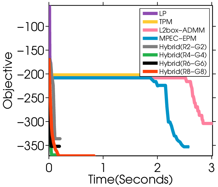
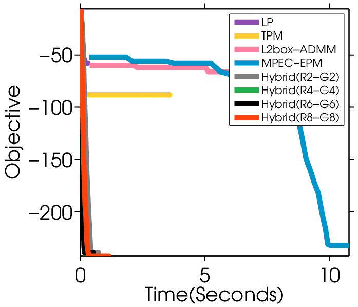
Compared Methods.We compare our HYBRID method on eight datasets (refer to the sub-captions in Figure 10)⁶⁶ 6 https://snap.stanford.edu/data/ against six methods: (i) LP relaxation (Yuan and Ghanem, 2017). (ii) Feige’s greedy algorithm (GEIGE) (Feige et al., 2001). (iii) Truncated Power Method (TPM) ⁷⁷ 7 https://sites.google.com/site/xtyuan1980/publications (Yuan and Zhang, 2013). (iv) L2box-ADMM (Wu and Ghanem, 2016). (v) MPEC-EPM (Yuan and Ghanem, 2017). For more description of these methods, we refer to (Yuan and Ghanem, 2017). We show the average results of using 3 random initial points.

Experimental Results.Several observations can be drawn from Figure 10. (i) FEIGE generally fails to solve the dense subgraph discovery problem and it leads to solutions with low density. (ii) TPM gives better performance than state-of-the-art technique MPEC-EPM in some cases but it is unstable. (iii) Our proposed HYBRID generally outperforms all the compared methods.

7.1 Computational Efficiency of Algorithm 1

We show the convergence curve of different methods for binary optimization (see Figure 11) and sparse optimization (see Figure 12). Generally speaking, our HYBRID is effective and practical for large-scale discrete optimization. Although it takes longer time to converge than PPA and QPM, the computational time is acceptable and it generally takes less than 30 seconds to converge in all our instances. We think this computation time pays off as HYBRID achieves significantly higher accuracy than PPA and QPM. The main bottleneck of computation is on solving the small-sized subproblem using sub-exponential time $\mathcal{O}(2^{k})$ . The parameter $k$ in Algorithm 1 can be viewed as a tuning parameter to balance the efficacy and efficiency. One can further accelerate the algorithm using asynchronous parallelism or mini-batch optimization techniques.

8 Conclusions

This paper presents an effective and practical method for solving discrete optimization problems. Our method takes advantage of the effectiveness of combinatorial search and the efficiency of gradient descent. We also provided rigorous optimality analysis and convergence analysis for the proposed algorithm. The extensive experiments show that our method achieves state-of-the-art performance.

Appendix

The appendix section is organized as follows. Section A, B, and C present the convergence rate for binary optimization, sparse regularized optimization, and sparse constrained optimization, respectively.

Appendix A Convergence Rate for Binary Optimization

We now prove the convergence rate of Algorithm 1 for binary optimization with $h\triangleq f_{\text{binary}}$ . We define $\Pi(\bm{\mathbf{a}})\triangleq\arg\min_{\bm{\mathbf{x}}}\|\bm{\mathbf{x}}-\bm{\mathbf{a}}\|,~s.t.~\bm{\mathbf{x}}\in\{-1,+1\}^{n}$ . Our key technique is that when it holds that $\|\Pi(\bm{\mathbf{x}})-\bm{\mathbf{x}}\|_{2}\leq(1-\kappa)\|\Pi(\bar{\bm{\mathbf{x}}})-\bm{\mathbf{x}}\|_{2}$ with $0<\kappa<1$ for any $\bm{\mathbf{x}}$ , combining with the strongly convex property of $f(\cdot)$ , we can establish global Q-linear convergence rate of Algorithm 1. We remark that the strongly convexity assumption always holds for binary optimization, since one can append an additional term $\frac{\eta}{2}\|\bm{\mathbf{x}}\|_{2}^{2}$ to $f(\cdot)$ with sufficiently large $\eta$ .

The following lemmas are useful in our proof.

Lemma 6.

Assume that $f(\cdot)$ is $\alpha$ -strongly convex. The following inequality holds for any $\bm{\mathbf{x}}$ and $\bm{\mathbf{y}}$ :

\displaystyle\frac{\alpha^{2}}{4}\|\bm{\mathbf{y}}-\bm{\mathbf{x}}\|_{2}^{2}-\|\nabla f(\bm{\mathbf{x}})\|_{2}^{2}\leq-\frac{\alpha}{2}(f(\bm{\mathbf{x}})-f(\bm{\mathbf{y}}))

(17)

Proof.

Since $f(\cdot)$ is $\alpha$ -strongly convex, it holds that:

\displaystyle f(\bm{\mathbf{x}})-f(\bm{\mathbf{y}})\leq\langle\nabla f(\bm{\mathbf{x}}),\bm{\mathbf{x}}-\bm{\mathbf{y}}\rangle-\frac{\alpha}{2}\|\bm{\mathbf{x}}-\bm{\mathbf{y}}\|_{2}^{2},~\forall\bm{\mathbf{x}},~\bm{\mathbf{y}}

(18)

We naturally derive the following results:

$\displaystyle\\|\nabla f(\bm{\mathbf{x}})\\|_{2}^{2}-\frac{\alpha^{2}}{4}\\|\bm{\mathbf{y}}-\bm{\mathbf{x}}\\|_{2}^{2}$	$\displaystyle=$	$\displaystyle\left(\\|\nabla f(\bm{\mathbf{x}})\\|_{2}-\frac{\alpha}{2}\\|\bm{\mathbf{y}}-\bm{\mathbf{x}}\\|_{2}\right)\cdot\left(\\|\nabla f(\bm{\mathbf{x}})\\|_{2}+\frac{\alpha}{2}\\|\bm{\mathbf{y}}-\bm{\mathbf{x}}\\|_{2}\right)$
	$\displaystyle\overset{}{\geq}$	$\displaystyle\left(\\|\nabla f(\bm{\mathbf{x}})\\|_{2}-\frac{\alpha}{2}\\|\bm{\mathbf{y}}-\bm{\mathbf{x}}\\|_{2}\right)\cdot\left(0+\frac{\alpha}{2}\\|\bm{\mathbf{y}}-\bm{\mathbf{x}}\\|_{2}\right)$
	$\displaystyle=$	$\displaystyle\frac{\alpha}{2}\left(\\|\nabla f(\bm{\mathbf{x}})\\|_{2}\cdot\\|\bm{\mathbf{y}}-\bm{\mathbf{x}}\\|_{2}-\frac{\alpha}{2}\\|\bm{\mathbf{y}}-\bm{\mathbf{x}}\\|_{2}^{2}\right)$
	$\displaystyle\overset{(a)}{\geq}$	$\displaystyle\frac{\alpha}{2}\left(\langle\nabla f(\bm{\mathbf{x}}),\bm{\mathbf{y}}-\bm{\mathbf{x}}\rangle-\frac{\alpha}{2}\\|\bm{\mathbf{y}}-\bm{\mathbf{x}}\\|_{2}^{2}\right)\overset{(b)}{\geq}\frac{\alpha}{2}(f(\bm{\mathbf{x}})-f(\bm{\mathbf{y}}))$

where step $(a)$ uses the Cauchy-Schwarz inequality; step $(b)$ uses the $\alpha$ -strongly convexity condition in (18).

∎

Lemma 7.

We define $\Pi(\bm{\mathbf{a}})=\arg\min_{\bm{\mathbf{x}}}\|\bm{\mathbf{x}}-\bm{\mathbf{a}}\|,~s.t.~\bm{\mathbf{x}}\in\{-1,+1\}^{n}$ . The following inequality always holds for all $\bm{\mathbf{x}}$ and $\bm{\mathbf{y}}$ :

\displaystyle\|\Pi(\bm{\mathbf{x}})-\bm{\mathbf{x}}\|_{2}^{2}\leq(1-\kappa)\|\Pi(\bm{\mathbf{y}})-\bm{\mathbf{x}}\|_{2}^{2}

(19)

with $\kappa=0$ . In addition, if $\Pi(\bm{\mathbf{x}}_{i})\neq\Pi(\bm{\mathbf{y}}_{i})$ and $\bm{\mathbf{x}}_{i}\neq 0$ for some $i$ , there exists a sufficiently small positive parameter $\kappa$ with $0<\kappa<1$ such that (19) holds.

Proof.

(i) First of all, noticing $\|\Pi(\bm{\mathbf{x}})\|_{2}^{2}=n$ for all $\bm{\mathbf{x}}$ , we have the following results:

			$\displaystyle\\|\Pi(\bm{\mathbf{x}})-\bm{\mathbf{x}}\\|_{2}^{2}\leq(1-\kappa)\\|\Pi(y)-\bm{\mathbf{x}}\\|_{2}^{2}$
		$\displaystyle\Leftrightarrow$	$\displaystyle\kappa\\|\Pi(y)-\bm{\mathbf{x}}\\|_{2}^{2}+\\|\Pi(\bm{\mathbf{x}})\\|_{2}^{2}+\\|\bm{\mathbf{x}}\\|_{2}^{2}-2\langle\Pi(\bm{\mathbf{x}}),\bm{\mathbf{x}}\rangle\leq\\|\Pi(y)\\|_{2}^{2}+\\|\bm{\mathbf{x}}\\|_{2}^{2}-2\langle\Pi(y),\bm{\mathbf{x}}\rangle$
		$\displaystyle\Leftrightarrow$	$\displaystyle\kappa\\|\Pi(y)-\bm{\mathbf{x}}\\|_{2}^{2}\leq 2\langle\Pi(x)-\Pi(y),\bm{\mathbf{x}}\rangle$

Since we have $\bm{\mathbf{x}}_{i}\cdot sign(\bm{\mathbf{y}}_{i})\leq\bm{\mathbf{x}}_{i}\cdot sign(\bm{\mathbf{x}}_{i})$ for all $i$ , the conclusion of this lemma clearly holds when $\kappa=0$ .

(ii) We now focus on the second part of this lemma. Note that $\Pi(\bm{\mathbf{x}})\neq\Pi(\bm{\mathbf{y}})$ also implies $\bm{\mathbf{x}}\neq\Pi(\bm{\mathbf{y}})$ and we have $\|\Pi(y)-\bm{\mathbf{x}}\|_{2}^{2}>0$ . Moreover, Therefore, there exists a sufficient small $\kappa$ such that $\kappa\|\Pi(y)-\bm{\mathbf{x}}\|_{2}^{2}\leq 2\langle\Pi(x)-\Pi(y),\bm{\mathbf{x}}\rangle$ holds. This finishes the proof of this lemma.

∎

Assumption 1.

Assuming that there exists a constant $0<\kappa<1$ such that:

\displaystyle\|\Pi(\bm{\mathbf{x}})-\bm{\mathbf{x}}\|^{2}_{2}\leq(1-\kappa)\|\bar{\bm{\mathbf{x}}}-\bm{\mathbf{x}}\|^{2}_{2},~\forall\bm{\mathbf{x}}

Remarks.Based on the results in Lemma 7, we conclude that when $\Pi(\bm{\mathbf{x}}_{i})\neq\Pi(\bar{\bm{\mathbf{x}}}_{i})$ and $\bm{\mathbf{x}}_{i}\neq 0$ for some $i$ , such an assumption holds. This constant is similar to the classical local proximal error bound constant (Luo and Tseng, 1993) and it is necessary to use this constant to characterize the global linear convergence rate of the algorithm.

Theorem 2.

Proof of Convergence Rate when $h\triangleq f_{\text{binary}}$ . When Assumption 1 holds and $f(\cdot)$ is $s$ -strongly convex, we have:

\displaystyle F(\bm{\mathbf{x}}^{t})-F(\bar{\bm{\mathbf{x}}})\leq(1-\beta)^{t}(F(\bm{\mathbf{x}}^{0})-F(\bar{\bm{\mathbf{x}}})),~~\text{with}~~\beta\triangleq(1-\kappa+\frac{\sqrt{{(L+\theta-s)(1-\kappa)\kappa}}}{2(L+\theta)})\frac{k}{n}<1

(20)

In other words, it takes at most $\log_{(1-\beta)}(\frac{\epsilon}{F(\bm{\mathbf{x}}^{0})-F(\bar{\bm{\mathbf{x}}})})$ times to find a solution $\bm{\mathbf{x}}^{t}$ satisfying $F(\bm{\mathbf{x}}^{t})-F(\bar{\bm{\mathbf{x}}})\leq\epsilon$ .

Proof.

First of all, we define

\displaystyle\textstyle d(\bm{\mathbf{x}})\triangleq\arg\min_{\bm{\mathbf{z}}\in\mathbb{R}^{n}}H(\bm{\mathbf{x}},\bm{\mathbf{z}}),~H(\bm{\mathbf{x}},\bm{\mathbf{z}})\triangleq f(\bm{\mathbf{x}})+\langle\nabla f(\bm{\mathbf{x}}),\bm{\mathbf{z}}\rangle+\frac{L+\theta}{2}\|\bm{\mathbf{z}}\|_{2}^{2}+h_{\text{binary}}(\bm{\mathbf{x}}+\bm{\mathbf{z}}).

Since $\bm{\mathbf{x}}^{t}\in\Psi$ for all $t$ . We have the following inequalities:

$\displaystyle\mathbb{E}[f(\bm{\mathbf{x}}^{t+1})]$	$\displaystyle\overset{(a)}{\leq}$	$\displaystyle\textstyle\mathbb{E}[f(\bm{\mathbf{z}})]+\frac{\theta}{2}\\|\bm{\mathbf{z}}-\bm{\mathbf{x}}^{t}\\|_{2}^{2}-\frac{\theta}{2}\\|\bm{\mathbf{x}}^{t+1}-\bm{\mathbf{x}}^{t}\\|_{2}^{2},~\forall\bm{\mathbf{z}}_{N}=\bm{\mathbf{x}}_{N}^{t},~\bm{\mathbf{z}}\in\Psi$	(21)
	$\displaystyle\overset{(b)}{\leq}$	$\displaystyle\textstyle\mathbb{E}[f(\bm{\mathbf{z}})]+\frac{\theta}{2}\\|\bm{\mathbf{z}}-\bm{\mathbf{x}}^{t}\\|_{2}^{2},~\forall\bm{\mathbf{z}}_{N}=\bm{\mathbf{x}}_{N}^{t},~\bm{\mathbf{z}}\in\Psi$
	$\displaystyle\overset{(c)}{\leq}$	$\displaystyle\textstyle\mathbb{E}[f(\bm{\mathbf{x}}^{t})+\langle\nabla f(\bm{\mathbf{x}}^{t}),~\bm{\mathbf{z}}-\bm{\mathbf{x}}^{t}\rangle+\frac{L}{2}\\|\bm{\mathbf{z}}-\bm{\mathbf{x}}^{t}\\|_{2}^{2}+\frac{\theta}{2}\\|\bm{\mathbf{z}}-\bm{\mathbf{x}}^{t}\\|_{2}^{2}],~\forall\bm{\mathbf{z}}_{N}=\bm{\mathbf{x}}_{N}^{t},~\bm{\mathbf{z}}\in\Psi$
	$\displaystyle\overset{(d)}{=}$	$\displaystyle\textstyle f(\bm{\mathbf{x}}^{t})+\mathbb{E}[\langle(\nabla f(\bm{\mathbf{x}}^{t}))_{B},~\bm{\mathbf{z}}_{B}-\bm{\mathbf{x}}_{B}^{t}\rangle]+\frac{L+\theta}{2}\mathbb{E}[\\|\bm{\mathbf{z}}_{B}-\bm{\mathbf{x}}^{t}_{B}\\|_{2}^{2}],~\bm{\mathbf{z}}\in\Psi$
	$\displaystyle\overset{(e)}{\leq}$	$\displaystyle\textstyle f(\bm{\mathbf{x}}^{t})+\mathbb{E}[\langle(\nabla f(\bm{\mathbf{x}}^{t}))_{B},~(\bm{\mathbf{x}}^{t}+d(\bm{\mathbf{x}}^{t}))_{B}-\bm{\mathbf{x}}_{B}^{t}\rangle]+\frac{L+\theta}{2}\mathbb{E}[\\|(\bm{\mathbf{x}}^{t}+d(\bm{\mathbf{x}}^{t}))_{B}-\bm{\mathbf{x}}^{t}_{B}\\|_{2}^{2}],~\bm{\mathbf{z}}\in\Psi$
	$\displaystyle\overset{(f)}{=}$	$\displaystyle\textstyle f(\bm{\mathbf{x}}^{t})+\frac{k}{n}\langle\nabla f(\bm{\mathbf{x}}^{t}),~d(\bm{\mathbf{x}}^{t})\rangle+\frac{k}{n}\frac{L+\theta}{2}\\|d(\bm{\mathbf{x}}^{t})\\|_{2}^{2}$

where step $(a)$ uses the optimality condition of $\bm{\mathbf{x}}^{t+1}$ ; step $(b)$ uses the fact that $-\frac{\theta}{2}\|\bm{\mathbf{x}}^{t+1}-\bm{\mathbf{x}}^{t}\|_{2}^{2}\leq 0$ ; step $(c)$ uses the Lipschitz continuity of the gradient of $f(\cdot)$ that: $f(\bm{\mathbf{z}})\leq f(\bm{\mathbf{x}})+\langle\nabla f(\bm{\mathbf{x}}),~\bm{\mathbf{z}}-\bm{\mathbf{x}}\rangle+\frac{L}{2}\|\bm{\mathbf{x}}-\bm{\mathbf{z}}\|_{2}^{2},~\forall\bm{\mathbf{x}},~\bm{\mathbf{z}}$ ; step $(d)$ uses the fact that $\bm{\mathbf{z}}_{N}=\bm{\mathbf{x}}_{N}^{t}$ ; step (e) uses the choice that $\bm{\mathbf{z}}=\bm{\mathbf{x}}+d(\bm{\mathbf{x}})$ ; step $(f)$ uses the fact that each block $B$ is picked randomly with probability $k/n$ .

We denotes

\displaystyle\breve{\bm{\mathbf{x}}}^{t}\triangleq\bm{\mathbf{x}}^{t}-\nabla f(\bm{\mathbf{x}}^{t})/(L+\theta).

(22)

For any $\bm{\mathbf{x}}^{t}\in\Psi$ and $\bm{\mathbf{x}}^{t+1}\in\Psi$ , we naturally derive the following inequalities:

	$\displaystyle\mathbb{E}[\frac{n}{k}F(\bm{\mathbf{x}}^{t+1})-\frac{n}{k}F(\bm{\mathbf{x}}^{t})]$	(23)
$\displaystyle\overset{(a)}{\leq}$	$\displaystyle\mathbb{E}[\langle\nabla f(\bm{\mathbf{x}}^{t}),d(\bm{\mathbf{x}}^{t})\rangle+\frac{L+\theta}{2}\\|d(\bm{\mathbf{x}}^{t})\\|_{2}^{2}]$
$\displaystyle\overset{(b)}{=}$	$\displaystyle\mathbb{E}[\langle\nabla f(\bm{\mathbf{x}}^{t}),\Pi\left(\bm{\mathbf{x}}^{t}-\nabla f(\bm{\mathbf{x}}^{t})/(L+\theta)\right)-\bm{\mathbf{x}}^{t}\rangle+\frac{L+\theta}{2}\\|\Pi\left(\bm{\mathbf{x}}^{t}-\nabla f(\bm{\mathbf{x}}^{t})/(L+\theta)\right)-\bm{\mathbf{x}}^{t}\\|_{2}^{2}]$
$\displaystyle\overset{(c)}{=}$	$\displaystyle\mathbb{E}[\langle\nabla f(\bm{\mathbf{x}}^{t}),\Pi(\breve{\bm{\mathbf{x}}}^{t})-\bm{\mathbf{x}}^{t}\rangle+\frac{L+\theta}{2}\\|\Pi(\breve{\bm{\mathbf{x}}}^{t})-\bm{\mathbf{x}}^{t}\\|_{2}^{2}]$
$\displaystyle\overset{(d)}{=}$	$\displaystyle\mathbb{E}[\frac{L+\theta}{2}\\|\Pi\left(\breve{\bm{\mathbf{x}}}^{t}\right)-\breve{\bm{\mathbf{x}}}^{t}\\|_{2}^{2}-\frac{L+\theta}{2}\\|\nabla f(\bm{\mathbf{x}}^{t})/(L+\theta)\\|_{2}^{2}]$

where step $(a)$ uses (21); step $(b)$ uses the fact that $d(\bm{\mathbf{x}})$ has the following closed-form solution that $d(\bm{\mathbf{x}})=\Pi\left(\bm{\mathbf{x}}-\frac{\nabla f(\bm{\mathbf{x}})}{L+\theta}\right)-\bm{\mathbf{x}}$ for any $\bm{\mathbf{x}}$ ; step $(c)$ uses the definition of $\breve{\bm{\mathbf{x}}}^{t}$ in (22); step $(d)$ the inequality that $\frac{t}{2}\|\bm{\mathbf{x}}\|_{2}^{2}+\langle\bm{\mathbf{x}},~\bm{\mathbf{a}}\rangle=\frac{t}{2}\|\bm{\mathbf{x}}+\bm{\mathbf{a}}/t\|_{2}^{2}-\frac{t}{2}\|\bm{\mathbf{a}}/t\|_{2}^{2}$ for all $\bm{\mathbf{a}},~\bm{\mathbf{x}},~t$ .

Based on Assumption 1, we have the following important inequality:

\displaystyle\|\Pi\left(\breve{\bm{\mathbf{x}}}^{t}\right)-\breve{\bm{\mathbf{x}}}^{t}\|_{2}^{2}\leq(1-\kappa)\|\Pi(\bar{\bm{\mathbf{x}}})-\breve{\bm{\mathbf{x}}}^{t}\|_{2}^{2}

(24)

We now bound the inequality in (23). We derive the following results:

	$\displaystyle\mathbb{E}[\frac{n}{k}F(\bm{\mathbf{x}}^{t+1})-\frac{n}{k}F(\bm{\mathbf{x}}^{t})]$	(25)
$\displaystyle\overset{(a)}{\leq}$	$\displaystyle\mathbb{E}[\frac{(L+\theta)(1-\kappa)}{2}\\|\Pi(\bar{\bm{\mathbf{x}}})-\breve{\bm{\mathbf{x}}}^{t}\\|_{2}^{2}-\frac{L+\theta}{2}\\|\nabla f(\bm{\mathbf{x}}^{t})/(L+\theta)\\|_{2}^{2}]$
$\displaystyle\overset{(b)}{=}$	$\displaystyle\mathbb{E}[\frac{(L+\theta)(1-\kappa)}{2}\\|\bar{\bm{\mathbf{x}}}-\bm{\mathbf{x}}^{t}+\nabla f(\bm{\mathbf{x}}^{t})/(L+\theta)\\|_{2}^{2}-\frac{L+\theta}{2}\\|\nabla f(\bm{\mathbf{x}}^{t})/(L+\theta)\\|_{2}^{2}]$
$\displaystyle\overset{}{=}$	$\displaystyle\mathbb{E}[\frac{(L+\theta)(1-\kappa)}{2}\\|\bar{\bm{\mathbf{x}}}-\bm{\mathbf{x}}^{t}\\|_{2}^{2}+(1-\kappa)\langle\bar{\bm{\mathbf{x}}}-\bm{\mathbf{x}}^{t},\nabla f(\bm{\mathbf{x}}^{t})\rangle-\frac{\kappa}{2}\\|\nabla f(\bm{\mathbf{x}}^{t})/(L+\theta)\\|_{2}^{2}]$
$\displaystyle\overset{(c)}{\leq}$	$\displaystyle\mathbb{E}[\frac{(L+\theta-s)(1-\kappa)}{2}\\|\bar{\bm{\mathbf{x}}}-\bm{\mathbf{x}}^{t}\\|_{2}^{2}+(1-\kappa)(f(\bar{\bm{\mathbf{x}}})-f(\bm{\mathbf{x}}^{t}))-\frac{\kappa}{2}\\|\nabla f(\bm{\mathbf{x}}^{t})/(L+\theta)\\|_{2}^{2}]$
$\displaystyle\overset{(d)}{=}$	$\displaystyle\mathbb{E}[(\frac{\kappa}{2(L+\theta)^{2}})(\frac{(L+\theta-s)(1-\kappa)(L+\theta)^{2}}{\kappa}\\|\bar{\bm{\mathbf{x}}}-\bm{\mathbf{x}}^{t}\\|_{2}^{2}-\\|\nabla f(\bm{\mathbf{x}}^{t})\\|_{2}^{2})+(1-\kappa)(f(\bar{\bm{\mathbf{x}}})-f(\bm{\mathbf{x}}^{t}))]$
$\displaystyle\overset{(e)}{\leq}$	$\displaystyle\mathbb{E}[(\frac{\kappa}{2(L+\theta)^{2}})\sqrt{\frac{(L+\theta-s)(1-\kappa)(L+\theta)^{2}}{\kappa}}(-f(\bm{\mathbf{x}}^{t})+f(\bar{\bm{\mathbf{x}}}))+(1-\kappa)(f(\bar{\bm{\mathbf{x}}})-f(\bm{\mathbf{x}}^{t}))]$
$\displaystyle\overset{}{=}$	$\displaystyle\mathbb{E}[(1-\kappa+\frac{\sqrt{{(L+\theta-s)(1-\kappa)\kappa}}}{2(L+\theta)})(f(\bar{\bm{\mathbf{x}}})-f(\bm{\mathbf{x}}^{t}))]$

step $(a)$ uses (24); step $(b)$ uses the fact that $\Pi(\bar{\bm{\mathbf{x}}})=\bar{\bm{\mathbf{x}}}$ and the definition of $\breve{\bm{\mathbf{x}}}^{t}$ in (22); step $(c)$ uses the $s$ -strongly convexity of $f(\cdot)$ that $\langle\bar{\bm{\mathbf{x}}}-\bm{\mathbf{x}}^{t},\nabla f(\bm{\mathbf{x}}^{t})\rangle\leq f(\bar{\bm{\mathbf{x}}})-f(\bm{\mathbf{x}}^{t})-\frac{s}{2}\|\bar{\bm{\mathbf{x}}}-\bm{\mathbf{x}}^{t}\|_{2}^{2}$ ; step $(e)$ uses the inequality in (17). It it worthwhile to note that when Assumption 1 does not hold with $\kappa\rightarrow 0$ , step $(d)$ breaks down.

Based on (25) and the definition of $\beta$ in (20), we have the following inequality: $\mathbb{E}[F(\bm{\mathbf{x}}^{t+1})-F(\bm{\mathbf{x}}^{t})]\leq\beta\mathbb{E}[F(\bar{\bm{\mathbf{x}}})-F(\bm{\mathbf{x}}^{t})]$ . Rearranging terms, we obtain that $\mathbb{E}[F(\bm{\mathbf{x}}^{t+1})-F(\bar{\bm{\mathbf{x}}})]\leq\mathbb{E}[(1-\beta)(F(\bm{\mathbf{x}}^{t})-F(\bar{\bm{\mathbf{x}})})]$ . In other words, the sequence $\{f(\bm{\mathbf{x}}^{t})\}$ converges to the stationary point linearly in the quotient sense. Solving this recursive formulation, we obtain (20). Therefore, we conclude that it takes at most $\log_{(1-\beta)}(\frac{\epsilon}{F(\bm{\mathbf{x}}^{0})-F(\bar{\bm{\mathbf{x}}})})$ times to find a local optimal solution satisfying $F(\bm{\mathbf{x}}^{t})-F(\bar{\bm{\mathbf{x}}})\leq\epsilon$ .

∎

Appendix B Convergence Rate for Sparse Regularized Optimization

We now prove the convergence rate of Algorithm 1 for sparse regularized optimization with $h\triangleq f_{\text{sparse}}$ . We have derived the upper bound for the number of changes $J$ for the support set in Theorem 5. We now need to derive a bound on the number of iterations performed after the support set is fixed. By combing these two bounds, we establish our proof.

The following lemma is useful in our proof.

Lemma 3.

Assume a nonnegative sequence $\{u^{t}\}_{t=0}^{\infty}$ satisfies $(u^{t+1})^{2}\leq C(u^{t}-u^{t+1})$ for some constant $C$ . We have:

\displaystyle u^{t}\leq\frac{\max(2C,\sqrt{Cu^{0}})}{t}

(26)

Proof.

We denote $C_{1}\triangleq\max(2C,\sqrt{Cu^{0}})$ . Solving this quadratic inequality, we have:

\displaystyle u^{t+1}\leq-\frac{C}{2}+\frac{C}{2}\sqrt{1+\frac{4u^{t}}{C}}

(27)

We now show that $u^{t+1}\leq\frac{C_{1}}{t+1}$ , which can be obtained by mathematical induction. (i) When $t=0$ , we have $u^{1}\leq-\frac{C}{2}+\frac{C}{2}\sqrt{1+\frac{4u^{0}}{C}}\leq-\frac{C}{2}+\frac{C}{2}(1+\sqrt{\frac{4u^{0}}{C}})=\frac{C}{2}\sqrt{\frac{4u^{0}}{C}}=\sqrt{Cu^{0}}\leq\frac{C_{1}}{t+1}$ . (ii) When $t\geq 1$ , we assume that $u^{t}\leq\frac{C_{1}}{t}$ holds. We derive the following results: $t\geq 1\Rightarrow\frac{t+1}{t}\leq 2$ $~\overset{(a)}{\Rightarrow}~C\frac{t+1}{t}\leq C_{1}$ $~\overset{(b)}{\Rightarrow}~$ $C(\frac{1}{t}-\frac{1}{t+1})\leq\frac{C_{1}}{(t+1)^{2}}$ $\Rightarrow\frac{C}{t}\leq\frac{C}{t+1}+\frac{C_{1}}{(t+1)^{2}}$ $\Rightarrow\frac{CC_{1}}{t}\leq\frac{CC_{1}}{t+1}+\frac{C^{2}_{1}}{(t+1)^{2}}$ $\Rightarrow\frac{C^{2}}{4}+\frac{CC_{1}}{t}\leq\frac{CC_{1}}{t+1}+\frac{C^{2}_{1}}{(t+1)^{2}}+\frac{C^{2}}{4}$ $\Rightarrow\frac{C^{2}}{4}(1+\frac{4C_{1}}{Ct})\leq(\frac{C}{2}+\frac{C_{1}}{t+1})^{2}$ $\Rightarrow\frac{C}{2}\sqrt{1+\frac{4C_{1}}{Ct}}\leq\frac{C}{2}+\frac{C_{1}}{t+1}$ $\Rightarrow-\frac{C}{2}+\frac{C}{2}\sqrt{1+\frac{4C_{1}}{Ct}}\leq\frac{C_{1}}{t+1}$ $~\overset{(c)}{\Rightarrow}~-\frac{C}{2}+\frac{C}{2}\sqrt{1+\frac{4u^{t}}{C}}\leq\frac{C_{1}}{t+1}$ $\Rightarrow u^{t+1}\leq\frac{C_{1}}{t+1}$ . Here, step $(a)$ uses $2C\leq C_{1}$ ; step $(b)$ uses $\frac{1}{t(t+1)}=\frac{1}{t}-\frac{1}{t+1}$ ; step $(c)$ uses $u^{t}\leq\frac{C_{1}}{t}$ .

∎

The following proposition establishes a bound on the number of iterations performed after the support set is fixed, which is novel in this paper. Note that the optimization problems become convex with fixing support set, and any stationary point $\bar{\bm{\mathbf{x}}}$ is also the global optimal solution for the convex problems.

Proposition 4.

Assume that the support set of $\bm{\mathbf{x}}^{t}$ does not changes for all $t$ . We have the following results:

(i) When $f(\cdot)$ is convex, it takes at most $V_{1}$ iterations in expectation for Algorithm 1 to converge to a stationary point $\bar{\bm{\mathbf{x}}}$ satisfying $F(\bm{\mathbf{x}}^{t})-F(\bar{\bm{\mathbf{x}}})\leq\epsilon$ , where $V_{1}$ is defined as:

\displaystyle V_{1}=\frac{\max(\frac{4\nu^{2}}{\theta},\sqrt{\frac{2\nu^{2}[F(\bm{\mathbf{x}}^{0})-F(\bar{\bm{\mathbf{x}}})]}{\theta}})}{\epsilon},~\text{with}~\nu\triangleq\frac{2n\rho\sqrt{k}\theta}{k}.

(28)

(ii) When $f(\cdot)$ is $s$ -strongly convex, it takes at most $V_{2}$ iterations in expectation for Algorithm 1 to converge to a stationary point $\bar{\bm{\mathbf{x}}}$ satisfying $F(\bm{\mathbf{x}}^{t})-F(\bar{\bm{\mathbf{x}}})\leq\epsilon$ , where $V_{2}$ is defined as:

\displaystyle V_{2}=\log_{\frac{\varpi}{1+\varpi}}(\frac{\epsilon}{F(\bm{\mathbf{x}}^{0})-F(\bar{\bm{\mathbf{x}}})}),~\text{with}~\varpi\triangleq\frac{\theta n}{sk}.

(29)

Proof.

First of all, we notice that when the support set is fixed, the original problem reduces to the following convex composite optimization problem:

\displaystyle\textstyle F(\bm{\mathbf{x}})\triangleq f(\bm{\mathbf{x}})+p(\bm{\mathbf{x}})+const,~~~\text{with}~~~p(\bm{\mathbf{x}})\triangleq I_{\Omega}(\bm{\mathbf{x}})

(30)

We use $\partial F(\bm{\mathbf{x}})$ to denote the sub-gradient of $F(\cdot)$ in $\bm{\mathbf{x}}$ . Since the algorithm solves the following optimization: $\bm{\mathbf{x}}^{t+1}\Leftarrow\arg\min_{\bm{\mathbf{z}}}~f(\bm{\mathbf{z}})+p(\bm{\mathbf{z}})+\frac{\theta}{2}\|\bm{\mathbf{z}}-\bm{\mathbf{x}}^{t}\|^{2},~s.t.~\bm{\mathbf{z}}_{N}=\bm{\mathbf{x}}^{t}_{N}$ , we have the following optimality condition for $\bm{\mathbf{x}}^{t+1}$ :

\displaystyle\bm{\mathbf{w}}_{B}+\theta(\bm{\mathbf{x}}^{t+1}-\bm{\mathbf{x}}^{t})_{B}=\bm{\mathbf{0}},~\bm{\mathbf{x}}^{t+1}_{N}=\bm{\mathbf{x}}^{t}_{N},~\forall\bm{\mathbf{w}}\in\partial F(\bm{\mathbf{x}}^{t+1})

(31)

(i) We now consider the case when $f(\cdot)$ is generally convex. We derive the following inequalities:

$\displaystyle\mathbb{E}[F(\bm{\mathbf{x}}^{t+1})]-F(\bar{\bm{\mathbf{x}}})$	$\displaystyle\overset{(a)}{\leq}$	$\displaystyle\mathbb{E}[\langle\bm{\mathbf{w}},\bm{\mathbf{x}}^{t+1}-\bar{\bm{\mathbf{x}}}\rangle],~\forall\bm{\mathbf{w}}\in\partial F(\bm{\mathbf{x}}^{t+1})$	(32)
	$\displaystyle\overset{(b)}{\leq}$	$\displaystyle\mathbb{E}[\frac{n}{k}\langle\bm{\mathbf{w}}_{B},(\bm{\mathbf{x}}^{t+1}-\bar{\bm{\mathbf{x}}})_{B}\rangle],~\forall\bm{\mathbf{w}}\in\partial F(\bm{\mathbf{x}}^{t+1})$
	$\displaystyle\overset{(c)}{=}$	$\displaystyle\mathbb{E}[\frac{n}{k}\langle-\theta(\bm{\mathbf{x}}^{t+1}-\bm{\mathbf{x}}^{t})_{B},(\bm{\mathbf{x}}^{t+1}-\bar{\bm{\mathbf{x}}})_{B}\rangle]$
	$\displaystyle\overset{(d)}{\leq}$	$\displaystyle\mathbb{E}[\frac{n}{k}\theta\\|(\bm{\mathbf{x}}^{t+1}-\bm{\mathbf{x}}^{t})_{B}\\|_{2}\cdot\\|(\bm{\mathbf{x}}^{t+1}-\bar{\bm{\mathbf{x}}})_{B}\\|_{2}]$
	$\displaystyle\overset{(e)}{=}$	$\displaystyle\mathbb{E}[\frac{n}{k}\theta\\|(\bm{\mathbf{x}}^{t+1}-\bm{\mathbf{x}}^{t})\\|_{2}\cdot\\|(\bm{\mathbf{x}}^{t+1}-\bar{\bm{\mathbf{x}}})_{B}\\|_{2}]$
	$\displaystyle\overset{(f)}{\leq}$	$\displaystyle\mathbb{E}[\underbrace{\frac{n}{k}\theta\cdot{2\rho}{\sqrt{k}}}_{\nu}\\|\bm{\mathbf{x}}^{t+1}-\bm{\mathbf{x}}^{t}\\|_{2}]$

where step $(a)$ uses the convexity of $F$ ; step $(b)$ uses the fact that each block $B$ is picked randomly with probability $k/n$ ; step $(c)$ uses the optimality condition of $\bm{\mathbf{x}}^{t+1}$ in (31); step $(d)$ uses the Cauchy-Schwarz inequality; step $(e)$ uses $\|(\bm{\mathbf{x}}^{t+1}-\bm{\mathbf{x}}^{t})\|_{2}=\|(\bm{\mathbf{x}}^{t+1}-\bm{\mathbf{x}}^{t})_{B}\|_{2}$ ; step $(f)$ uses $\|(\bm{\mathbf{x}}^{t+1}-\bar{\bm{\mathbf{x}}})_{B}\|\leq{\sqrt{k}}\|(\bm{\mathbf{x}}^{t+1}-\bar{\bm{\mathbf{x}}})_{B}\|_{\infty}\leq{\sqrt{k}}\|\bm{\mathbf{x}}^{t+1}-\bar{\bm{\mathbf{x}}}\|_{\infty}\leq{\sqrt{k}}(\|\bm{\mathbf{x}}^{t+1}\|_{\infty}+\|\bar{\bm{\mathbf{x}}}\|_{\infty})\leq{2\rho}{\sqrt{k}}$ .

For any $\bm{\mathbf{x}}^{t},\bm{\mathbf{x}}^{t+1},~\bar{\bm{\mathbf{x}}}~\in\Omega$ , we derive the following results:

\displaystyle\mathbb{E}[F(\bm{\mathbf{x}}^{t+1})-F(\bar{\bm{\mathbf{x}}})]\overset{(a)}{\leq}\mathbb{E}[\nu\|\bm{\mathbf{x}}^{t+1}-\bm{\mathbf{x}}^{t}\|_{2}]\overset{(b)}{\leq}\mathbb{E}[\nu\sqrt{\frac{2}{\theta}\left(F(\bm{\mathbf{x}}^{t})-F(\bm{\mathbf{x}}^{t+1})\right)}]

(33)

where the step $(a)$ uses (32); step $(b)$ uses the sufficient decent condition in (5). Denoting $\Delta^{t}\triangleq\mathbb{E}[F(\bm{\mathbf{x}}^{t})-F(\bar{\bm{\mathbf{x}}})]$ and $C\triangleq\frac{2\nu^{2}}{\theta}$ , we have the following inequality:

\displaystyle(\Delta^{t+1})^{2}\leq C(\Delta^{t}-\Delta^{t+1})

Combining with Lemma 3, we have:

\displaystyle\mathbb{E}[F(\bm{\mathbf{x}}^{t})-F(\bar{\bm{\mathbf{x}}})]\leq\frac{\max(\frac{4\nu^{2}}{\theta},\sqrt{\frac{2\nu^{2}\Delta^{0}}{\theta}})}{t}

Therefore, we obtain (28).

(ii) We now consider the case when $f(\cdot)$ is strongly convex. For any $\bm{\mathbf{x}}^{t},\bm{\mathbf{x}}^{t+1},~\bar{\bm{\mathbf{x}}}~\in\Omega$ , we derive the following results:

$\displaystyle\mathbb{E}[F(\bm{\mathbf{x}}^{t+1})-F(\bar{\bm{\mathbf{x}}})]$	$\displaystyle\overset{(a)}{\leq}$	$\displaystyle\mathbb{E}[-\frac{s}{2}\\|\bar{\bm{\mathbf{x}}}-\bm{\mathbf{x}}^{t+1}\\|_{2}^{2}-\langle\bar{\bm{\mathbf{x}}}-\bm{\mathbf{x}}^{t+1},\bm{\mathbf{w}}\rangle],~\forall\bm{\mathbf{w}}\in\partial F(\bm{\mathbf{x}}^{t+1})$	(34)
	$\displaystyle\overset{(b)}{\leq}$	$\displaystyle\mathbb{E}[\frac{1}{2s}\\|\bm{\mathbf{w}}\\|_{2}^{2}],~\forall\bm{\mathbf{w}}\in\partial F(\bm{\mathbf{x}}^{t+1})$
	$\displaystyle\overset{(c)}{=}$	$\displaystyle\mathbb{E}[-\frac{1}{2s}\\|\bm{\mathbf{w}}_{B}\\|_{2}^{2}\times\frac{n}{k}],~\forall\bm{\mathbf{w}}\in\partial F(\bm{\mathbf{x}}^{t+1})$
	$\displaystyle\overset{(d)}{=}$	$\displaystyle\mathbb{E}[-\frac{1}{2s}\\|\theta(\bm{\mathbf{x}}^{t+1}-\bm{\mathbf{x}}^{t})_{B}\\|_{2}^{2}\times\frac{n}{k}]$
	$\displaystyle\overset{}{=}$	$\displaystyle\mathbb{E}[\frac{\theta^{2}n}{2sk}\\|\bm{\mathbf{x}}^{t+1}-\bm{\mathbf{x}}^{t}\\|_{2}^{2}]$
	$\displaystyle\overset{(e)}{\leq}$	$\displaystyle\mathbb{E}[\frac{\theta^{2}n}{2sk}\frac{2}{\theta}\left(F(\bm{\mathbf{x}}^{t})-F(\bm{\mathbf{x}}^{t+1})]\right)$
	$\displaystyle\overset{}{=}$	$\displaystyle\mathbb{E}[\underbrace{\frac{\theta n}{sk}}_{\varpi}\left([F(\bm{\mathbf{x}}^{t})-F(\bar{\bm{\mathbf{x}}})]-[F(\bm{\mathbf{x}}^{t+1})-F(\bar{\bm{\mathbf{x}}})]\right)]$

where step $(a)$ uses the strongly convexity of $f(\cdot)$ ; step $(b)$ uses the fact that $-\frac{s}{2}\|\bm{\mathbf{x}}\|_{2}^{2}-\langle\bm{\mathbf{x}},\bm{\mathbf{y}}\rangle\leq\frac{1}{2s}\|\bm{\mathbf{y}}\|_{2}^{2}$ ; step $(c)$ uses the fact that $\mathbb{E}[\|\bm{\mathbf{w}}_{B}\|_{2}^{2}]=\frac{k}{n}\|\bm{\mathbf{w}}\|_{2}^{2}$ ; step $(d)$ uses the optimality of $\bm{\mathbf{x}}^{t+1}$ ; step $(e)$ uses the sufficient condition in $(\ref{eq:suff:dec})$ .

Rearranging terms for (34), we have: $\frac{\mathbb{E}[F(\bm{\mathbf{x}}^{t+1})-F(\bar{\bm{\mathbf{x}}})]}{\mathbb{E}[F(\bm{\mathbf{x}}^{t})-F(\bar{\bm{\mathbf{x}}})]}\leq\frac{\varpi}{1+\varpi}$ . Solving the recursive formulation, we obtain:

\displaystyle\mathbb{E}[F(\bm{\mathbf{x}}^{t})-F(\bar{\bm{\mathbf{x}}})]\leq\mathbb{E}[\left(\frac{\varpi}{1+\varpi}\right)^{t}[F(\bm{\mathbf{x}}^{0})-F(\bar{\bm{\mathbf{x}}})]],

and it holds that $t\leq\log_{\frac{\varpi}{1+\varpi}}\left(\frac{F(\bm{\mathbf{x}}^{t})-F(\bar{\bm{\mathbf{x}}})}{F(\bm{\mathbf{x}}^{0})-F(\bar{\bm{\mathbf{x}}})}\right)$ in expectation. Therefore, we obtain (29).

∎

Theorem 3.

Convergence Rate when $h\triangleq f_{\text{sparse}}$ . We have the follow results:

(i) When $f(\cdot)$ is generally convex, it takes at most $N_{1}$ iterations in expectation to converge to a block- $k$ stationary point $\bar{\bm{\mathbf{x}}}$ such that $F(\bm{\mathbf{x}}^{t})-F(\bar{\bm{\mathbf{x}}})\leq\epsilon$ , where

\displaystyle N_{1}=\left(\frac{\bar{J}}{D}+\frac{1}{\epsilon}\right)\times\max\left(\frac{4\nu^{2}}{\theta},\sqrt{\frac{2\nu^{2}(F(\bm{\mathbf{x}}^{0})-F(\bar{\bm{\mathbf{x}}})-D)}{\theta}}\right).

(ii) When $f(\cdot)$ is $s$ -strongly convex, it takes at most $N_{2}$ iterations in expectation to converge to a block- $k$ stationary point $\bar{\bm{\mathbf{x}}}$ such that $F(\bm{\mathbf{x}}^{t})-F(\bar{\bm{\mathbf{x}}})\leq\epsilon$ , where

\displaystyle N_{2}=\bar{J}\log_{\frac{\varpi}{1+\varpi}}\left(\frac{D}{(F(\bm{\mathbf{x}}^{0})-F(\bar{\bm{\mathbf{x}}}))}\right)+\log_{\frac{\varpi}{1+\varpi}}\left(\frac{\epsilon}{F(\bm{\mathbf{x}}^{0})-D-F(\bar{\bm{\mathbf{x}}})}\right).

(35)

Proof.

(i) We first consider the case when $f(\cdot)$ is generally convex. We denote $Z_{t}=\{i:\bm{\mathbf{x}}^{t}_{i}=0\}$ . We known that the $Z_{t}$ only changes for a finite number of times. We assume that $Z_{t}$ only changes at $t=c_{1},c_{2},...,c_{\bar{J}}$ and we define $c_{0}=0$ . Therefore, we have:

\displaystyle Z_{0}=Z_{1}=,...,Z_{-1+c_{1}}\neq Z_{c_{1}}=Z_{1+c_{1}}=Z_{2+c_{1}}=,...,=Z_{-1+c_{j}}\neq Z_{c_{j}}=...\neq Z_{c_{{\bar{J}}}}=...

with $j=1,...,{\bar{J}}$ . We denote $\bar{\bm{\mathbf{x}}}^{c_{j}}$ as the optimal solution of the following optimization problem:

\displaystyle\min_{\bm{\mathbf{x}}}~f(\bm{\mathbf{x}})+p(\bm{\mathbf{x}}),~s.t.~\bm{\mathbf{x}}_{I_{c_{j}}}=0

(36)

with $1\leq j\leq{\bar{J}}$ .

The solution $\bm{\mathbf{x}}^{c_{j}}$ changes $j$ times, the objective values decrease at least by $jD$ , where $D$ is defined in (13). Therefore, we have:

\displaystyle F(\bm{\mathbf{x}}^{c_{j}})\leq F(\bm{\mathbf{x}}^{0})-{j}\times D

Combing with the fact that $F(\bar{\bm{\mathbf{x}}})\leq F(\bar{\bm{\mathbf{x}}}^{c_{j}})$ , we obtain:

\displaystyle 0\leq F(\bm{\mathbf{x}}^{c_{j}})-F(\bar{\bm{\mathbf{x}}}^{c_{j}})\leq F(\bm{\mathbf{x}}^{0})-F(\bar{\bm{\mathbf{x}}})-j\times D

(37)

We now focus on the intermediate solutions $\bm{\mathbf{x}}_{c_{j-1}},~\bm{\mathbf{x}}_{1+c_{j-1}},...,~\bm{\mathbf{x}}_{-1+c_{j}},\bm{\mathbf{x}}_{c_{j}}$ . Using part (i) in Proposition 4, we conclude that to obtain an accuracy such that $F(\bm{\mathbf{x}}^{c_{j}})-F(\bar{\bm{\mathbf{x}}}^{c_{j}})\leq D$ , it takes at most ${\max\left(\frac{4\nu^{2}}{\theta},\sqrt{\frac{2\nu^{2}(F(\bm{\mathbf{x}}^{c_{j}})-F(\bar{\bm{\mathbf{x}}}^{c_{j}}))}{\theta}}\right)}/{D}$ iterations to converge to $\bar{\bm{\mathbf{x}}}^{c_{j}}$ , that is,

\displaystyle c_{j}-c_{j-1}\leq\frac{\max\left(\frac{4\nu^{2}}{\theta},\sqrt{\frac{2\nu^{2}(F(\bm{\mathbf{x}}^{c_{j}})-F(\bar{\bm{\mathbf{x}}}^{c_{j}}))}{\theta}}\right)}{D}\leq\frac{\max\left(\frac{4\nu^{2}}{\theta},\sqrt{\frac{2\nu^{2}(F(\bm{\mathbf{x}}^{0})-F(\bar{\bm{\mathbf{x}}})-j\times D)}{\theta}}\right)}{D}

(38)

Summing up the inequality in (38) for $j=1,2,...,\bar{J}$ and using the fact that $j\geq 1$ and $c_{0}=0$ , we obtain that:

\displaystyle c_{{\bar{J}}}\leq\bar{J}\times\frac{\max\left(\frac{4\nu^{2}}{\theta},\sqrt{\frac{2\nu^{2}(F(\bm{\mathbf{x}}^{0})-F(\bar{\bm{\mathbf{x}}})-D)}{\theta}}\right)}{D}

(39)

After $c_{\bar{J}}$ iterations, Algorithm 1 becomes the proximal gradient method applied to the problem as in (36). Therefore, the total number of iterations for finding a block- $k$ stationary point $N_{1}$ is bounded by:

$\displaystyle N_{1}$	$\displaystyle\overset{(a)}{\leq}$	$\displaystyle c_{\bar{J}}+\frac{\max(\frac{4\nu^{2}}{\theta},\sqrt{\frac{2\nu^{2}[F(\bm{\mathbf{x}}^{c_{\bar{J}}})-F(\bar{\bm{\mathbf{x}}})]}{\theta}})}{\epsilon}$
	$\displaystyle\overset{(b)}{\leq}$	$\displaystyle c_{\bar{J}}+\frac{\max(\frac{4\nu^{2}}{\theta},\sqrt{\frac{2\nu^{2}[F(\bm{\mathbf{x}}^{0})-F(\bar{\bm{\mathbf{x}}})-D]}{\theta}})}{\epsilon}$
	$\displaystyle\overset{}{=}$	$\displaystyle\left(\frac{\bar{J}}{D}+\frac{1}{\epsilon}\right)\times\max\left(\frac{4\nu^{2}}{\theta},\sqrt{\frac{2\nu^{2}(F(\bm{\mathbf{x}}^{0})-F(\bar{\bm{\mathbf{x}}})-D)}{\theta}}\right)$

where step $(a)$ uses the fact that the total number of iterations for finding a stationary point after $\bm{\mathbf{x}}_{c_{\bar{J}}}$ is upper bounded by ${\max(\frac{4\nu^{2}}{\theta},\sqrt{\frac{2\nu^{2}[F(\bm{\mathbf{x}}^{c_{\bar{J}}})-F(\bar{\bm{\mathbf{x}}})]}{\theta}})}/{\epsilon}$ ; step $(b)$ uses (37) and $j\geq 1$ .

(ii) We now discuss the case when $f(\cdot)$ is strongly convex. Using part (ii) in Proposition 4, we have:

\displaystyle c_{j}-c_{j-1}\leq\log_{\frac{\varpi}{1+\varpi}}\frac{D}{F(\bm{\mathbf{x}}^{0})-F(\bar{\bm{\mathbf{x}}})},

(40)

Summing up the inequality (40) for $j=1,2,...,\bar{J}$ , we obtain the following results:

\displaystyle c_{{\bar{J}}}\leq\log_{\frac{\varpi}{1+\varpi}}\left(\frac{D^{\bar{J}}}{(F(\bm{\mathbf{x}}^{0})-F(\bar{\bm{\mathbf{x}}}))^{\bar{J}}}\right)=\bar{J}\log_{\frac{\varpi}{1+\varpi}}\left(\frac{D}{(F(\bm{\mathbf{x}}^{0})-F(\bar{\bm{\mathbf{x}}}))}\right)

Therefore, the total number of iterations $N_{2}$ is bounded by:

	$\displaystyle N_{2}$	$\displaystyle\overset{(a)}{\leq}$	$\displaystyle c_{\bar{J}}+\log_{\frac{\varpi}{1+\varpi}}\left(\frac{\epsilon}{F(\bm{\mathbf{x}}^{c_{\bar{J}}})-F(\bar{\bm{\mathbf{x}}})}\right)$
		$\displaystyle\overset{(b)}{\leq}$	$\displaystyle c_{\bar{J}}+\log_{\frac{\varpi}{1+\varpi}}\left(\frac{\epsilon}{F(\bm{\mathbf{x}}^{0})-D-F(\bar{\bm{\mathbf{x}}})}\right)$

where step $(a)$ uses the fact that the total number of iterations for finding a stationary point after $\bm{\mathbf{x}}_{c_{\bar{J}}}$ is upper bounded by $\log_{\frac{\varpi}{1+\varpi}}\left(\frac{\epsilon}{F(\bm{\mathbf{x}}^{c_{\bar{J}}})-F(\bar{\bm{\mathbf{x}}})}\right)$ ; step $(b)$ uses (37) that $0\leq F(\bm{\mathbf{x}}^{0})-F(\bar{\bm{\mathbf{x}}})-t\times D$ and $t\geq 1$ .

∎

Appendix C Convergence Rate for Sparsity Constrained Optimization

We now prove the convergence rate of Algorithm 1 for sparse constrained optimization with $h\triangleq f_{\text{sparse-c}}$ . We results are based on the strongly convex and Lipschitz continuity of the objective function. We naturally derive the following theorem.

Theorem 4.

Proof of Convergence Rate when $h\triangleq f_{\text{sparse-c}}$ . Let $f(\cdot)$ be an $s$ -strongly convex function. We assume that $f(\cdot)$ is Lipschitz continuous such that $\forall t,~\|\nabla f(\bm{\mathbf{x}}^{t})\|_{2}^{2}\leq M$ for some constant $M$ . We have the following results:

	$\displaystyle\mathbb{E}[F(\bm{\mathbf{x}}^{t})-F(\bar{\bm{\mathbf{x}}})]$	$\displaystyle\leq$	$\displaystyle(F(\bm{\mathbf{x}}^{0})-F(\bar{\bm{\mathbf{x}}}))\alpha^{t}+\frac{M}{2\theta}\frac{\alpha}{1-\alpha},~$
	$\displaystyle\mathbb{E}[\frac{s}{4}\\|\bm{\mathbf{x}}^{t+1}-\bar{\bm{\mathbf{x}}}\\|^{2}_{2}]$	$\displaystyle\leq$	$\displaystyle\frac{n2\theta}{k}(F(\bm{\mathbf{x}}^{0})-F(\bar{\bm{\mathbf{x}}}))\alpha^{t}+\frac{n}{k}\frac{M}{1-\alpha},~\text{with}~\alpha\triangleq\frac{\frac{n\theta}{ks}}{1+\frac{n\theta}{ks}}.$

Proof.

(i) First of all, we define the zero set and nonzero set as follows:

\displaystyle S\triangleq\{i~|~i\in B,~\bm{\mathbf{x}}_{i}^{t+1}\neq 0\},~Z\triangleq\{i~|~i\in B,~\bm{\mathbf{x}}_{i}^{t+1}=0\},~

Using the optimality of $\bm{\mathbf{x}}^{t+1}$ for the subproblem, we obtain

\displaystyle(\nabla f(\bm{\mathbf{x}}^{t+1}))_{S}+\theta(\bm{\mathbf{x}}^{t+1}_{S}-\bm{\mathbf{x}}^{t}_{S})=0~\Rightarrow~(\nabla f(\bm{\mathbf{x}}^{t+1}))_{S}/\theta+\bm{\mathbf{x}}^{t+1}_{S}=\bm{\mathbf{x}}^{t}_{S}

(41)

We derive the following inequalities:

	$\displaystyle\mathbb{E}[f(\bm{\mathbf{x}}^{t+1})-f(\bar{\bm{\mathbf{x}}})]$	(42)
$\displaystyle\overset{(a)}{\leq}$	$\displaystyle\mathbb{E}[\langle\bm{\mathbf{x}}^{t+1}-\bar{\bm{\mathbf{x}}},~\nabla f(\bm{\mathbf{x}}^{t+1})\rangle-\frac{s}{2}\\|\bm{\mathbf{x}}^{t+1}-\bar{\bm{\mathbf{x}}}\\|_{2}^{2}]$
$\displaystyle\overset{(b)}{=}$	$\displaystyle\frac{n}{k}\cdot\mathbb{E}[\langle\bm{\mathbf{x}}_{B}^{t+1}-\bm{\mathbf{x}}_{B}^{*},~(\nabla f(\bm{\mathbf{x}}^{t+1}))_{B}\rangle-\frac{s}{2}\\|\bm{\mathbf{x}}^{t+1}_{B}-\bar{\bm{\mathbf{x}}}_{B}\\|_{2}^{2}]$
$\displaystyle\overset{(c)}{\leq}$	$\displaystyle\frac{n}{k}\cdot\frac{s}{2}\cdot\mathbb{E}[\\|(\nabla f(\bm{\mathbf{x}}^{t+1}))_{B}/s\\|_{2}^{2}]$
$\displaystyle\overset{(d)}{=}$	$\displaystyle\frac{n}{k}\cdot\frac{s}{2}\cdot\left(\mathbb{E}[\\|(\nabla f(\bm{\mathbf{x}}^{t+1}))_{S}/s\\|_{2}^{2}]+\mathbb{E}[\\|(\nabla f(\bm{\mathbf{x}}^{t+1}))_{Z}/s\\|_{2}^{2}]\right)$
$\displaystyle\overset{(e)}{\leq}$	$\displaystyle\mathbb{E}[\frac{n}{k}\frac{s}{2}\cdot[\\|\theta(\bm{\mathbf{x}}_{S}^{t}-\bm{\mathbf{x}}^{t+1}_{S})/s\\|_{2}^{2}+\\|(\nabla f(\bm{\mathbf{x}}^{t+1}))_{Z}/s\\|_{2}^{2}]]$
$\displaystyle\overset{(f)}{\leq}$	$\displaystyle\mathbb{E}[\frac{n}{k}\frac{\theta}{s}\cdot\frac{\theta}{2}\\|\bm{\mathbf{x}}^{t}-\bm{\mathbf{x}}^{t+1}\\|_{2}^{2}+\frac{n}{k}\frac{s}{2}\\|(\nabla f(\bm{\mathbf{x}}^{t+1}))_{Z}/s\\|_{2}^{2}]$
$\displaystyle\overset{(g)}{\leq}$	$\displaystyle\mathbb{E}[\frac{n}{k}\frac{\theta}{s}\cdot[f(\bm{\mathbf{x}}^{t})-f(\bm{\mathbf{x}}^{t+1})]+\frac{n}{k}\frac{1}{2s}\\|(\nabla f(\bm{\mathbf{x}}^{t+1}))_{Z}\\|_{2}^{2}]$
$\displaystyle\overset{(h)}{\leq}$	$\displaystyle\mathbb{E}[\frac{n}{k}\frac{\theta}{s}\cdot(f(\bm{\mathbf{x}}^{t})-f(\bar{\bm{\mathbf{x}}}))-\frac{n}{k}\frac{\theta}{s}\cdot(f(\bm{\mathbf{x}}^{t+1})-f(\bar{\bm{\mathbf{x}}}))+\frac{n}{k}\frac{1}{2s}\cdot M]$

where step $(a)$ uses the strongly convexity of $f(\cdot)$ ; step $(b)$ uses the fact that the working set $B$ is selected with $\frac{k}{n}$ probability; step $(c)$ uses the inequality that $\langle\bm{\mathbf{x}},~\bm{\mathbf{a}}\rangle-\frac{s}{2}\|\bm{\mathbf{x}}\|_{2}^{2}=\frac{s}{2}\|\bm{\mathbf{a}}/s\|_{2}^{2}-\frac{s}{2}\|\bm{\mathbf{x}}-\bm{\mathbf{a}}/s\|_{2}^{2}\leq\frac{s}{2}\|\bm{\mathbf{a}}/s\|_{2}^{2}$ for all $\bm{\mathbf{a}},~\bm{\mathbf{x}}$ ; step $(d)$ uses the fact that $B=S\cup Z$ , step $(e)$ uses (41); step $(f)$ uses $\|\bm{\mathbf{x}}_{S}\|_{2}^{2}\leq\|\bm{\mathbf{x}}\|_{2}^{2}$ for all $\bm{\mathbf{x}}$ ; step $(g)$ uses the sufficient decrease condition that $\frac{\theta}{2}\|\bm{\mathbf{x}}^{t+1}-\bm{\mathbf{x}}^{t}\|^{2}\leq F(\bm{\mathbf{x}}^{t})-F(\bm{\mathbf{x}}^{t+1})$ ; step $(h)$ uses the Lipschitz continuity of $f(\cdot)$ that $\|\nabla f(\bm{\mathbf{x}}^{t+1})\|_{2}^{2}\leq M,~\forall t$ .

From (42), we have the following inequalities:

	$\displaystyle\mathbb{E}[(1+\frac{n\theta}{ks})(f(\bm{\mathbf{x}}^{t+1})-f(\bar{\bm{\mathbf{x}}}))]\leq\mathbb{E}[\frac{n\theta}{ks}\cdot(f(\bm{\mathbf{x}}^{t})-f(\bar{\bm{\mathbf{x}}}))+\frac{nM}{2ks}]$
	$\displaystyle\mathbb{E}[f(\bm{\mathbf{x}}^{t+1})-f(\bar{\bm{\mathbf{x}}})]\leq\mathbb{E}[\alpha(f(\bm{\mathbf{x}}^{t})-f(\bar{\bm{\mathbf{x}}}))+\frac{\frac{n}{2ks}}{\frac{n}{k}\frac{\theta}{s}}\alpha M]$
	$\displaystyle\mathbb{E}[f(\bm{\mathbf{x}}^{t+1})-f(\bar{\bm{\mathbf{x}}})]\leq\mathbb{E}[\alpha(f(\bm{\mathbf{x}}^{t})-f(\bar{\bm{\mathbf{x}}}))+\frac{\alpha M}{2\theta}]$

Solving this recursive formulation, we have:

$\displaystyle\mathbb{E}[f(\bm{\mathbf{x}}^{t})-f(\bar{\bm{\mathbf{x}}})]$	$\displaystyle\leq$	$\displaystyle\mathbb{E}[\alpha^{t}(f(\bm{\mathbf{x}}^{0})-f(\bar{\bm{\mathbf{x}}}))]+M\sum_{i=1}^{t}\alpha^{i}$
	$\displaystyle=$	$\displaystyle\mathbb{E}[\alpha^{t}(f(\bm{\mathbf{x}}^{0})-f(\bar{\bm{\mathbf{x}}}))]+\frac{M\alpha}{2\theta}\cdot\frac{1-\alpha^{t}}{1-\alpha}$
	$\displaystyle\leq$	$\displaystyle\mathbb{E}[\alpha^{t}(f(\bm{\mathbf{x}}^{0})-f(\bar{\bm{\mathbf{x}}}))]+\frac{M}{2\theta}\cdot\frac{\alpha}{1-\alpha}$

Since $\bm{\mathbf{x}}^{t}$ is always a feasible solution for all $t=1,2,...\infty$ , we have $F(\bm{\mathbf{x}}^{t})=f(\bm{\mathbf{x}}^{t})$ . Therefore, we obtain (4).

(ii) We now prove the second part of this theorem. First, we derive the following inequalities:

$\displaystyle\mathbb{E}[\\|\bm{\mathbf{x}}^{t+1}-\bm{\mathbf{x}}^{t}\\|_{2}^{2}]$	$\displaystyle\overset{(a)}{\leq}$	$\displaystyle\mathbb{E}[\frac{2}{\theta}\left(F(\bm{\mathbf{x}}^{t})-F(\bm{\mathbf{x}}^{t+1})\right)]$	(43)
	$\displaystyle\overset{(b)}{\leq}$	$\displaystyle\mathbb{E}[\frac{2}{\theta}\left(F(\bm{\mathbf{x}}^{t})-F(\bar{\bm{\mathbf{x}}})\right)]$
	$\displaystyle\overset{(c)}{\leq}$	$\displaystyle\mathbb{E}[\frac{2}{\theta}\alpha^{t}(f(\bm{\mathbf{x}}^{0})-f(\bar{\bm{\mathbf{x}}}))]+\frac{M}{\theta^{2}}\cdot\frac{\alpha}{1-\alpha}$

where step $(a)$ uses the sufficient decrease condition in (5); step $(b)$ uses the fact that $F(\bar{\bm{\mathbf{x}}})\leq F({\bm{\mathbf{x}}}^{t+1})$ ; step $(c)$ uses the result in (4).

Second, we have the following results:

$\displaystyle\mathbb{E}[\frac{s}{2}\\|\bm{\mathbf{x}}^{t+1}-\bar{\bm{\mathbf{x}}}\\|_{2}^{2}]$	$\displaystyle\overset{(a)}{\leq}$	$\displaystyle\mathbb{E}[\langle\bm{\mathbf{x}}^{t+1}-\bar{\bm{\mathbf{x}}},~\nabla f(\bm{\mathbf{x}}^{t+1})\rangle+f(\bar{\bm{\mathbf{x}}})-f(\bm{\mathbf{x}}^{t+1})]$	(44)
	$\displaystyle\overset{(b)}{\leq}$	$\displaystyle\mathbb{E}[\langle\bm{\mathbf{x}}^{t+1}-\bar{\bm{\mathbf{x}}},~\nabla f(\bm{\mathbf{x}}^{t+1})\rangle]$
	$\displaystyle\overset{(c)}{\leq}$	$\displaystyle\mathbb{E}[\\|\bm{\mathbf{x}}^{t+1}-\bar{\bm{\mathbf{x}}}\\|\cdot\\|\nabla f(\bm{\mathbf{x}}^{t+1})\\|]$

where step $(a)$ uses the strongly convexity of $f(\cdot)$ ; step $(b)$ uses the fact that $f(\bar{\bm{\mathbf{x}}})\leq f({\bm{\mathbf{x}}}^{t+1})$ ; step $(c)$ uses the Cauchy-Schwarz inequality.

From (44), we further have the following results:

$\displaystyle\mathbb{E}[\frac{s}{4}\\|\bm{\mathbf{x}}^{t+1}-\bar{\bm{\mathbf{x}}}\\|^{2}_{2}]$	$\displaystyle\overset{(a)}{\leq}$	$\displaystyle\mathbb{E}[\\|\nabla f(\bm{\mathbf{x}}^{t+1})\\|_{2}^{2}]$
	$\displaystyle\overset{}{=}$	$\displaystyle\frac{n}{k}\mathbb{E}[\\|\nabla_{B}f(\bm{\mathbf{x}}^{t+1})\\|_{2}^{2}]$
	$\displaystyle\overset{(b)}{=}$	$\displaystyle\frac{n}{k}\mathbb{E}[\\|\nabla_{S}f(\bm{\mathbf{x}}^{t+1})\\|_{2}^{2}+\\|\nabla_{Z}f(\bm{\mathbf{x}}^{t+1})\\|_{2}^{2}]$
	$\displaystyle\overset{(c)}{\leq}$	$\displaystyle\frac{n}{k}\mathbb{E}[\theta^{2}\\|\bm{\mathbf{x}}^{t+1}_{S}-\bm{\mathbf{x}}^{t}_{S}\\|_{2}^{2}]+\frac{n}{k}M$
	$\displaystyle\overset{(d)}{=}$	$\displaystyle\frac{n}{k}\mathbb{E}[{2\theta}\alpha^{t}(f(\bm{\mathbf{x}}^{0})-f(\bar{\bm{\mathbf{x}}}))+\frac{M}{1-\alpha}]$

where step $(a)$ uses the strongly convexity of $f(\cdot)$ ; step $(b)$ uses the fact that $B=S\cup Z$ ; step $(c)$ uses the assumption that $\|\nabla f(\bm{\mathbf{x}}^{t})\|_{2}^{2}\leq M$ for all $\bm{\mathbf{x}}^{t}$ and the optimality of $\bm{\mathbf{x}}^{t+1}$ in (41); step $(d)$ uses (43). Therefore, we finish the proof of this theorem.

∎

References

Aharon et al. (2006) Michal Aharon, Michael Elad, and Alfred Bruckstein. K-svd: An algorithm for designing overcomplete dictionaries for sparse representation. IEEE Transactions on Signal Processing, 54(11):4311–4322, 2006.
Bao et al. (2016) Chenglong Bao, Hui Ji, Yuhui Quan, and Zuowei Shen. Dictionary learning for sparse coding: Algorithms and convergence analysis. IEEE Transactions on Pattern Analysis and Machine Intelligence (TPAMI), 38(7):1356–1369, 2016.
Beck and Eldar (2013) Amir Beck and Yonina C Eldar. Sparsity constrained nonlinear optimization: Optimality conditions and algorithms. SIAM Journal on Optimization (SIOPT), 23(3):1480–1509, 2013.
Beck and Teboulle (2009) Amir Beck and Marc Teboulle. A fast iterative shrinkage-thresholding algorithm for linear inverse problems. SIAM Journal on Imaging Sciences (SIIMS), 2(1):183–202, 2009.
Beck and Tetruashvili (2013) Amir Beck and Luba Tetruashvili. On the convergence of block coordinate descent type methods. SIAM Journal on Optimization (SIOPT), 23(4):2037–2060, 2013.
Bienstock (1996) Daniel Bienstock. Computational study of a family of mixed-integer quadratic programming problems. Mathematical Programming, 74(2):121–140, 1996.
Blumensath and Davies (2008) Thomas Blumensath and Mike E Davies. Gradient pursuits. IEEE Transactions on Signal Processing, 56(6):2370–2382, 2008.
Boykov et al. (2001) Yuri Boykov, Olga Veksler, and Ramin Zabih. Fast approximate energy minimization via graph cuts. IEEE Transactions on Pattern Analysis and Machine Intelligence (TPAMI), 23(11):1222–1239, 2001.
Breheny and Huang (2011) Patrick Breheny and Jian Huang. Coordinate descent algorithms for nonconvex penalized regression, with applications to biological feature selection. The Annals of Applied Statistics, 5(1):232, 2011.
Călinescu et al. (2011) Gruia Călinescu, Chandra Chekuri, Martin Pál, and Jan Vondrák. Maximizing a monotone submodular function subject to a matroid constraint. SIAM Journal on Computing (SICOMP), 40(6):1740–1766, 2011.
Candes and Tao (2005) Emmanuel J Candes and Terence Tao. Decoding by linear programming. IEEE Transactions on Information Theory, 51(12):4203–4215, 2005.
Chang et al. (2008) Kai-Wei Chang, Cho-Jui Hsieh, and Chih-Jen Lin. Coordinate descent method for large-scale l2-loss linear support vector machines. Journal of Machine Learning Research (JMLR), 9(Jul):1369–1398, 2008.
Chen and Gu (2016) Jinghui Chen and Quanquan Gu. Accelerated stochastic block coordinate gradient descent for sparsity constrained nonconvex optimization. In Uncertainty in Artificial Intelligence (UAI), 2016.
Conforti et al. (2014) Michele Conforti, Gérard Cornuéjols, and Giacomo Zambelli. Integer programming, volume 271. Springer, 2014.
Dai and Milenkovic (2009) Wei Dai and Olgica Milenkovic. Subspace pursuit for compressive sensing signal reconstruction. IEEE Transactions on Information Theory, 55(5):2230–2249, 2009.
De Santis et al. (2016) Marianna De Santis, Stefano Lucidi, and Francesco Rinaldi. A fast active set block coordinate descent algorithm for $\backslash$ ell_1-regularized least squares. SIAM Journal on Optimization (SIOPT), 26(1):781–809, 2016.
Donoho (2006) David L. Donoho. Compressed sensing. IEEE Transactions on Information Theory, 52(4):1289–1306, 2006.
Elhamifar and Vidal (2013) Ehsan Elhamifar and Rene Vidal. Sparse subspace clustering: Algorithm, theory, and applications. IEEE Transactions on Pattern Analysis and Machine Intelligence (TPAMI), 35(11):2765–2781, 2013.
Feige et al. (2001) Uriel Feige, David Peleg, and Guy Kortsarz. The dense k-subgraph problem. Algorithmica, 29(3):410–421, 2001.
Hong et al. (2013) Mingyi Hong, Xiangfeng Wang, Meisam Razaviyayn, and Zhi-Quan Luo. Iteration complexity analysis of block coordinate descent methods. Mathematical Programming, pages 1–30, 2013.
Hsieh and Dhillon (2011) Cho-Jui Hsieh and Inderjit S Dhillon. Fast coordinate descent methods with variable selection for non-negative matrix factorization. In ACM International Conference on Knowledge Discovery and Data Mining (SIGKDD), pages 1064–1072, 2011.
Hsieh et al. (2008) Cho-Jui Hsieh, Kai-Wei Chang, Chih-Jen Lin, S Sathiya Keerthi, and Sellamanickam Sundararajan. A dual coordinate descent method for large-scale linear svm. In International Conference on Machine Learning (ICML), pages 408–415, 2008.
Jain et al. (2014) Prateek Jain, Ambuj Tewari, and Purushottam Kar. On iterative hard thresholding methods for high-dimensional m-estimation. In Neural Information Processing Systems (NIPS), pages 685–693, 2014.
Johnson and Zhang (2013) Rie Johnson and Tong Zhang. Accelerating stochastic gradient descent using predictive variance reduction. In Advances in Neural Information Processing Systems (NIPS), pages 315–323, 2013.
Li et al. (2016) Xingguo Li, Raman Arora, Han Liu, Jarvis Haupt, and Tuo Zhao. Nonconvex sparse learning via stochastic optimization with progressive variance reduction. arXiv Preprint, 2016.
Liu et al. (2015) Ji Liu, Stephen J Wright, Christopher Ré, Victor Bittorf, and Srikrishna Sridhar. An asynchronous parallel stochastic coordinate descent algorithm. Journal of Machine Learning Research (JMLR), 16(285-322):1–5, 2015.
Lu (2014) Zhaosong Lu. Iterative hard thresholding methods for $\ell_{0}$ regularized convex cone programming. Mathematical Programming, 147(1-2):125–154, 2014.
Lu and Xiao (2015) Zhaosong Lu and Lin Xiao. On the complexity analysis of randomized block-coordinate descent methods. Mathematical Programming, 152(1-2):615–642, 2015.
Lu and Zhang (2013) Zhaosong Lu and Yong Zhang. Sparse approximation via penalty decomposition methods. SIAM Journal on Optimization (SIOPT), 23(4):2448–2478, 2013.
Luo and Tseng (1993) Zhi-Quan Luo and Paul Tseng. Error bounds and convergence analysis of feasible descent methods: a general approach. Annals of Operations Research, 46(1):157–178, 1993.
Necoara (2013) Ion Necoara. Random coordinate descent algorithms for multi-agent convex optimization over networks. IEEE Transactions on Automatic Control, 58(8):2001–2012, 2013.
Needell and Tropp (2009) Deanna Needell and Joel A Tropp. Cosamp: Iterative signal recovery from incomplete and inaccurate samples. Applied and Computational Harmonic Analysis, 26(3):301–321, 2009.
Needell and Vershynin (2010) Deanna Needell and Roman Vershynin. Signal recovery from incomplete and inaccurate measurements via regularized orthogonal matching pursuit. IEEE Journal of Selected Topics in Signal Processing, 4(2):310–316, 2010.
Nesterov (2012) Yu Nesterov. Efficiency of coordinate descent methods on huge-scale optimization problems. SIAM Journal on Optimization (SIOPT), 22(2):341–362, 2012.
Nesterov (2013) Yurii Nesterov. Introductory lectures on convex optimization: A basic course, volume 87. Springer Science & Business Media, 2013.
Nguyen et al. (2014) Nam Nguyen, Deanna Needell, and Tina Woolf. Linear convergence of stochastic iterative greedy algorithms with sparse constraints. arXiv Preprint, 2014.
Patrascu and Necoara (2015a) Andrei Patrascu and Ion Necoara. Random coordinate descent methods for $\ell_{0}$ regularized convex optimization. IEEE Transactions on Automatic Control, 60(7):1811–1824, 2015a.
Patrascu and Necoara (2015b) Andrei Patrascu and Ion Necoara. Efficient random coordinate descent algorithms for large-scale structured nonconvex optimization. Journal of Global Optimization, 61(1):19–46, 2015b.
Powell (1973) M. J. D. Powell. On search directions for minimization algorithms. Mathematical Programming, 4(1):193–201, 1973.
Ravi et al. (1994) Sekharipuram S Ravi, Daniel J Rosenkrantz, and Giri K Tayi. Heuristic and special case algorithms for dispersion problems. Operations Research, 42(2):299–310, 1994.
Razaviyayn et al. (2013) Meisam Razaviyayn, Mingyi Hong, and Zhi-Quan Luo. A unified convergence analysis of block successive minimization methods for nonsmooth optimization. SIAM Journal on Optimization (SIOPT), 23(2):1126–1153, 2013.
Recht et al. (2011) Benjamin Recht, Christopher Re, Stephen Wright, and Feng Niu. Hogwild: A lock-free approach to parallelizing stochastic gradient descent. In Neural Information Processing Systems (NIPS), pages 693–701, 2011.
Tropp and Gilbert (2007) Joel A Tropp and Anna C Gilbert. Signal recovery from random measurements via orthogonal matching pursuit. IEEE Transactions on Information Theory, 53(12):4655–4666, 2007.
Tseng and Yun (2009) Paul Tseng and Sangwoon Yun. A coordinate gradient descent method for nonsmooth separable minimization. Mathematical Programming, 117(1):387–423, 2009.
Wang et al. (2018) Jingdong Wang, Ting Zhang, Jingkuan Song, Nicu Sebe, and Heng Tao Shen. A survey on learning to hash. IEEE Transactions on Pattern Analysis and Machine Intelligence (TPAMI), 40(4):769–790, 2018.
Wang et al. (2016) Jun Wang, Wei Liu, Sanjiv Kumar, and Shih-Fu Chang. Learning to hash for indexing big data - a survey. Proceedings of the IEEE, 104(1):34–57, 2016.
Wu and Ghanem (2016) Baoyuan Wu and Bernard Ghanem. $\ell_{p}$ -box admm: A versatile framework for integer programming. arXiv Preprint, 2016.
Xiao and Zhang (2014) Lin Xiao and Tong Zhang. A proximal stochastic gradient method with progressive variance reduction. SIAM Journal on Optimization (SIOPT), 24(4):2057–2075, 2014.
Xu and Yin (2013) Yangyang Xu and Wotao Yin. A block coordinate descent method for regularized multiconvex optimization with applications to nonnegative tensor factorization and completion. SIAM Journal on Imaging Sciences (SIIMS), 6(3):1758–1789, 2013.
Yuan and Ghanem (2017) Ganzhao Yuan and Bernard Ghanem. An exact penalty method for binary optimization based on MPEC formulation. In AAAI Conference on Artificial Intelligence (AAAI), pages 2867–2875, 2017.
Yuan et al. (2017) Ganzhao Yuan, Wei-Shi Zheng, and Bernard Ghanem. A matrix splitting method for composite function minimization. In IEEE Conference on Computer Vision and Pattern Recognition (CVPR), 2017.
Yuan and Zhang (2013) Xiao-Tong Yuan and Tong Zhang. Truncated power method for sparse eigenvalue problems. Journal of Machine Learning Research (JMLR), 14(Apr):899–925, 2013.
Zhang and Gu (2016) Aston Zhang and Quanquan Gu. Accelerated stochastic block coordinate descent with optimal sampling. In ACM International Conference on Knowledge Discovery and Data Mining (SIGKDD), pages 2035–2044, 2016.

$\displaystyle\\|\nabla f(\bm{\mathbf{x}})\\|_{2}^{2}-\frac{\alpha^{2}}{4}\\|\bm{\mathbf{y}}-\bm{\mathbf{x}}\\|_{2}^{2}$	$\displaystyle=$	$\displaystyle\left(\\|\nabla f(\bm{\mathbf{x}})\\|_{2}-\frac{\alpha}{2}\\|\bm{\mathbf{y}}-\bm{\mathbf{x}}\\|_{2}\right)\cdot\left(\\|\nabla f(\bm{\mathbf{x}})\\|_{2}+\frac{\alpha}{2}\\|\bm{\mathbf{y}}-\bm{\mathbf{x}}\\|_{2}\right)$
	$\displaystyle\overset{}{\geq}$	$\displaystyle\left(\\|\nabla f(\bm{\mathbf{x}})\\|_{2}-\frac{\alpha}{2}\\|\bm{\mathbf{y}}-\bm{\mathbf{x}}\\|_{2}\right)\cdot\left(0+\frac{\alpha}{2}\\|\bm{\mathbf{y}}-\bm{\mathbf{x}}\\|_{2}\right)$
	$\displaystyle=$	$\displaystyle\frac{\alpha}{2}\left(\\|\nabla f(\bm{\mathbf{x}})\\|_{2}\cdot\\|\bm{\mathbf{y}}-\bm{\mathbf{x}}\\|_{2}-\frac{\alpha}{2}\\|\bm{\mathbf{y}}-\bm{\mathbf{x}}\\|_{2}^{2}\right)$
	$\displaystyle\overset{(a)}{\geq}$	$\displaystyle\frac{\alpha}{2}\left(\langle\nabla f(\bm{\mathbf{x}}),\bm{\mathbf{y}}-\bm{\mathbf{x}}\rangle-\frac{\alpha}{2}\\|\bm{\mathbf{y}}-\bm{\mathbf{x}}\\|_{2}^{2}\right)\overset{(b)}{\geq}\frac{\alpha}{2}(f(\bm{\mathbf{x}})-f(\bm{\mathbf{y}}))$

			$\displaystyle\\|\Pi(\bm{\mathbf{x}})-\bm{\mathbf{x}}\\|_{2}^{2}\leq(1-\kappa)\\|\Pi(y)-\bm{\mathbf{x}}\\|_{2}^{2}$
		$\displaystyle\Leftrightarrow$	$\displaystyle\kappa\\|\Pi(y)-\bm{\mathbf{x}}\\|_{2}^{2}+\\|\Pi(\bm{\mathbf{x}})\\|_{2}^{2}+\\|\bm{\mathbf{x}}\\|_{2}^{2}-2\langle\Pi(\bm{\mathbf{x}}),\bm{\mathbf{x}}\rangle\leq\\|\Pi(y)\\|_{2}^{2}+\\|\bm{\mathbf{x}}\\|_{2}^{2}-2\langle\Pi(y),\bm{\mathbf{x}}\rangle$
		$\displaystyle\Leftrightarrow$	$\displaystyle\kappa\\|\Pi(y)-\bm{\mathbf{x}}\\|_{2}^{2}\leq 2\langle\Pi(x)-\Pi(y),\bm{\mathbf{x}}\rangle$