Sampling and Reconstruction in Distinct Subspaces Using Oblique ProjectionsThanks: Funding by the Austrian Science Fund (FWF) through grant NFN SISE (S10602) and P26273 - N25 and by the Vienna Science and Technology Fund (WWTF) through project VRG12-009 and project ICT15-119.

Peter Berger Address: Institute of Telecommunications
Vienna University of Technology,
Gusshausstrasse 25/389
A-1040 Vienna, Austria Email address: peter.berger@nt.tuwien.ac.at , Karlheinz Gröchenig Address: Faculty of Mathematics
University of Vienna
Oskar-Morgenstern-Platz 1
A-1090 Vienna, Austria Email address: karlheinz.groechenig@univie.ac.at and Gerald Matz Address: Institute of Telecommunications
Vienna University of Technology,
Gusshausstrasse 25/389
A-1040 Vienna, Austria Email address: gerald.matz@tuwien.ac.at

Abstract.

We study reconstruction operators on a Hilbert space that are exact on a given reconstruction subspace. Among those the reconstruction operator obtained by the least squares fit has the smallest operator norm, and therefore is most stable with respect to noisy measurements. We then construct the operator with the smallest possible quasi-optimality constant, which is the most stable with respect to a systematic error appearing before the sampling process (model uncertainty). We describe how to vary continuously between the two reconstruction methods, so that we can trade stability for quasi-optimality. As an application we study the reconstruction of a compactly supported function from nonuniform samples of its Fourier transform.

1. Introduction

1.1. The reconstruction problem

In this paper we treat the following sampling problem. Let $\mathcal{H}$ be a separable Hilbert space over $\mathbb{C}$ with inner product $\langle\cdot,\cdot\rangle_{\mathcal{H}}$ .We assume that we are given linear measurements $(\langle f,u_{j}\rangle_{\mathcal{H}})_{j\in\mathbb{N}}$ , $u_{j}\in\mathcal{H}$ , of an unknown function $f\in\mathcal{H}$ . We call $(u_{j})_{j\in\mathbb{N}}$ the sampling frame and $\mathcal{U}:=\overline{\textnormal{span}}(u_{j})_{j\in\mathbb{N}}$ the sampling space. Our goal is to approximate the function $f$ by an element in the reconstruction space $\mathcal{T}:=\overline{\textnormal{span}}(t_{k})_{k\in\mathbb{N}}$ with $t_{k}\in\mathcal{H}$ , by a series expansion $\tilde{f}=\sum_{k\in\mathbb{N}}c_{k}t_{k}$ from the given measurements. The main point is that in general the reconstruction space is distinct from the sampling space, whereas in classical frame theory these two spaces coincide.

1.2. Areas of application and related work

This type of sampling problem arises in many concrete applications and in the numerical modelling of infinite dimensional problems.

(i) Sampling of bandlimited functions. In [25] a bandlimited function is approximated from finitely many, nonuniform samples by means of a trigonometric polynomial. In this case the sampling space consists of the reproducing kernels $u_{j}(x)=\frac{\sin\pi(x-x_{j})}{\pi(x-x_{j})},j=1,\dots,n,$ and the reconstruction vectors are $t_{k}(x)=e^{2\pi ikx/(2M+1)}\chi_{[-M,M]}(x),|k|\leqslant M$ .

(ii) Inverse Polynomial Reconstruction Method. In this method one tries to approximate an algebraic polynomial or an analytic function from its Fourier samples. Thus the sampling space consists of vectors $u_{j}(x)=e^{\pi ijx}\chi_{[-1,1]}(x),j=1,\dots,m$ , and the reconstruction space consists of a suitable polynomial basis, usually the monomials $t_{k}(x)=x^{k},k=0,\dots,n$ , or the Legendre polynomials. This method claims to efficiently mitigate the Gibbs phenomenon [38, 28, 29, 30], and, indeed, the modified inverse polynomial reconstruction method [27] leads to a numerically stable reconstruction when $m\geqslant n^{2}$ .

(iii) Fourier sampling. More generally, the goal is to approximate a compactly supported function in some smoothness class from its nonuniform Fourier samples $\hat{f}(\omega_{j})$ . Thus the sampling space consists again of the functions $u_{j}(x)=e^{\pi i\omega_{j}x}\chi_{[-1,1]}(x)$ . The reconstruction space depends on the signal model and on a priori information. If $f$ is smooth and belongs to a Besov space, then the reconstruction space may be taken to be a wavelet subspace. The problems of Fourier sampling have motivated Adcock and Hansen to revisit nonuniform sampling theory and to create the impressive and useful framework of generalized sampling [8, 7, 10, 6, 33].

(iv) Model reduction in parametric partial differential equations and the generalized empirical interpolation method. In general the solution manifold to a parametric partial differential equation is quite complicated, therefore it is approximated by finite-dimensional spaces $\mathcal{T}_{n}$ . The GEIM (GEIM) [34, 35] builds an interpolant in an $n$ -dimensional space $\mathcal{T}_{n}$ based on the knowledge of $n$ physical measurements $(\langle f,u_{j}\rangle_{\mathcal{H}})_{j=1}^{n}$ . In [36, 13] an extension based on a least squares method has been proposed, where the dimension $m$ of $\mathcal{T}_{m}$ is smaller than the number $n$ of the measurements $(\langle f,u_{j}\rangle_{\mathcal{H}})_{j=1}^{n}$ . A further generalization to Banach spaces is contained in [18]. The focus in [36, 13] lies in minimizing the error caused by the model mismatch. This is done by using a correction term outside of the reconstruction space, which means that (in contrast to our work) the reconstruction is allowed to be located outside of the reconstruction space. This approach is optimal in the absence of measurement noise [13].

In all these problems the canonical approximation or reconstruction is by means of a least squares fit, namely

\tilde{f}=\underset{g\in\mathcal{T}}{\textnormal{arg~min}}\sum_{j\in\mathbb{N}}w_{j}\left|\langle g,u_{j}\rangle_{\mathcal{H}}-d_{j}\right|^{2}\,.

(1)

The weights $w_{j}$ are usually chosen to be $w_{j}=1$ , but in many contexts is has turned out to be useful to use weights as a kind of cheap preconditioners. The use of adaptive weights in sampling theory goes back at least to [23, 24], and has become standard in the recent work on (Fourier) sampling, see for example [5, 25, 26, 40, 1, 3, 2, 4, 11].

1.3. The reconstruction operators

In this paper we restrict ourselves to the case where the approximation $\tilde{f}=\sum_{k\in\mathbb{N}}c_{k}t_{k}$ of the unknown function $f\in\mathcal{H}$ is obtained by a linear and bounded reconstruction operator $Q:\ell^{2}(\mathbb{N})\rightarrow\mathcal{T}$ . Thus the approximation $\tilde{f}$ from the data $\langle f,u_{j}\rangle_{j\in\mathbb{N}}$ is given by $\tilde{f}=Q\big(\langle f,u_{j}\rangle_{j\in\mathbb{N}}\big)$ . We will use two quantities to measure the quality of such a reconstruction operator. As a measure of stability with respect to measurement noise we use the operator norm $\|Q\|_{\rm op}$ . As a measure of stability with respect to model mismatch we follow [9] and use the so-called quasi-optimality constant $\mu(Q)$ (see Definition 2.1).

Let $P_{\mathcal{T}}$ denote the orthogonal projection onto $\mathcal{T}$ , $f\in\mathcal{H}$ the target function, and $l\in\ell^{2}(\mathbb{N})$ be the noise vector. Then the input data are given by the sequence $(\langle f,u_{j}\rangle_{\mathcal{H}}+l_{j})_{j\in\mathbb{N}}$ , the reconstruction is $\tilde{f}=Q((\langle f,u_{j}\rangle_{\mathcal{H}}+l_{j})_{j\in\mathbb{N}})$ , and the error is bounded by

\|f-Q((\langle f,u_{j}\rangle_{\mathcal{H}}+l_{j})_{j\in\mathbb{N}})\|_{\mathcal{H}}\leqslant\mu(Q)\|f-P_{\mathcal{T}}f\|_{\mathcal{H}}+\|Q\|_{\rm op}\|l\|_{2}.

(2)

1.4. Contributions

The error bound (2) raises several questions:

•

Which operators admit an error bound of the form (2)?
•

Under what circumstances does such an operator exist?
•

Which operator has the smallest possible operator norm $\|Q\|_{\rm op}$ ?
•

Which operator has the smallest possible quasi-optimality constant $\mu(Q)$ ?
•

Is there a way to trade-off between quasi-optimality and operator norm?

Our objective is to answer these questions both in finite-dimensional and infinite dimensional Hilbert spaces. The results can be formulated conveniently in the language of frame theory.

(i) Characterization of all reconstruction operators. We characterize all reconstruction operators that admit an error estimate of the form (2). In fact, every dual frame of the set $(P_{\mathcal{T}}u_{j})_{j\in\mathbb{N}}$ yields a reconstruction satisfying (2). Conversely, every reconstruction operator subject to (2) is the synthesis operator of a dual frame of $(P_{\mathcal{T}}u_{j})_{j\in\mathbb{N}}$ . Note that (2) implies that such a reconstruction operator $Q$ is exact on the reconstruction space, i.e., $f=Q(\langle f,u_{j}\rangle_{\mathcal{H}})_{j\in\mathbb{N}}$ for all $f\in\mathcal{T}$ . Reconstruction operators fulfilling this property are called perfect. For a precise formulation see Theorem 2.2.

The important insight of [9] is the connection between stability and the angle $\phi_{\mathcal{T},\mathcal{U}}$ between the sampling space and the reconstruction space. We will see that a perfect reconstruction operator exists if and only if $\cos(\phi_{\mathcal{T},\mathcal{U}})>0$ . It should also be mentioned that the reconstruction operators considered in this paper are a special case of pseudoframes [32].

(ii) Least squares approximation. As already mentioned, the canonical approximation of the data $\langle f,u_{j}\rangle_{j\in\mathbb{N}}$ by a vector in $\mathcal{T}$ is by a least squares fit. Let $U^{*}f=(\langle f,u_{j}\rangle_{\mathcal{H}})_{j\in\mathbb{N}}$ denote the analysis operator of the frame $(u_{j})_{j\in\mathbb{N}}$ and let $d\in\ell^{2}(\mathbb{N})$ denote the vector containing the noisy measurements $(d_{j})=(\langle f,u_{j}\rangle_{\mathcal{H}}+l_{j})_{j\in\mathbb{N}}=U^{*}f+l$ . Let the reconstruction operator $Q_{1}$ be defined by the least squares fit

Q_{1}d=\underset{g\in\mathcal{T}}{\textnormal{arg~min}}\sum_{j\in\mathbb{N}}\left|\langle g,u_{j}\rangle_{\mathcal{H}}-d_{j}\right|^{2}=\underset{g\in\mathcal{T}}{\textnormal{arg~min}}\|U^{*}g-d\|_{2}.

(3)

It is folklore that the least squares solution (3) is optimal in the absence of additional information on $f$ . Precise formulations of this optimality were proven in [9, Theorem 6.2.] (including even non-linear reconstructions) and in [12] (in abstract Hilbert space). We will show in addition (Theorem 3.1) that $Q_{1}$ is the synthesis operator of the canonical dual frame of $(P_{\mathcal{T}}u_{j})_{j\in\mathbb{N}}$ . Using this property we derive a simple proof for the statement that the operator $Q_{1}$ has the smallest possible operator norm among all perfect reconstruction operators.

(iii) Minimizing the quasi-optimality constant. Let $W=G^{\frac{\dagger}{2}}:=(G^{\dagger})^{\frac{1}{2}}$ be the square root of the Moore-Penrose pseudoinverse of the Gramian $G=U^{*}U$ of the sampling frame $\mathcal{U}$ and consider the operator $Q_{0}$ defined by

Q_{0}d=\underset{g\in\mathcal{T}}{\textnormal{arg~min}}\|WU^{*}g-Wd\|_{2}\,.

(4)

We will show (Theorem 3.3) that $Q_{0}$ has the smallest possible quasi-optimality constant. The reduction of the quasi-optimality constant is one of the motivations of weighted least squares, see [2, 1, 5, 3]. In (4) we go a step further and use the non-diagonal matrix $W=G^{\frac{\dagger}{2}}$ as a weight for the least squares problem. From the point of view of linear algebra, $W$ may be seen as a preconditioner.

In [2, 1, 5, 3] and also [11, 24, 25, 26, 4, 23] the stability with respect to a bias in the measured object is considered, i.e., the reconstruction from $U^{*}(f+\Delta f)=(\langle f+\Delta f,u_{j}\rangle_{\mathcal{H}})_{j\in\mathbb{N}}$ (stated in terms of a frame inequality in the latter). In this context, $Q_{0}$ is the most stable operator with respect to biased objects, see the discussion in Section 3.6.

(iv) Trading stability and quasi-stability. It is natural to ask whether one can mix between the two least squares problems (3) and (4). Let $\Sigma_{\lambda}=\big(\lambda I+(1-\lambda)U^{*}U\big)$ and $\lambda\in[0,1]$ and define $Q_{\lambda}$ by

Q_{\lambda}d=\underset{g\in\mathcal{T}}{\textnormal{arg~min}}\|\Sigma_{\lambda}^{-\frac{1}{2}}U^{*}g-\Sigma_{\lambda}^{-\frac{1}{2}}d\|_{2}\,.

These reconstruction operators “interpolate” between $Q_{1}$ (most stable with respect to noise) and $Q_{0}$ (most stable with respect to model uncertainty). The parameter $\lambda$ can be seen as a regularization parameter, or alternatively the matrix $\Sigma_{\lambda}$ as version of the adaptive weights in sampling. In Theorem 3.7 and Lemma 3.8 we will study this class of reconstruction operators and derive several representations for $Q_{\lambda}$ .

(v) Fourier resampling — numerical experiments. In the last part we carry out a numerical comparison of the various reconstruction operators on the basis of the so-called resampling problem. We approximate a function with compact support from finitely many, nonuniform samples of its Fourier transform and then resample the Fourier transform on a regular grid. For this problem we test the performance of the reconstruction operators $Q_{\lambda}$ .

The paper is organized as follows: In Section 2 we introduce the frame theoretic background, discuss the angle between subspaces, and characterize all reconstruction operators satisfying the required stability estimate (2). In Section 3 we study the various least squares problems (3) and (4) and analyze several representations of the corresponding reconstruction operators. The section is complemented by general numerical considerations. Section 4 covers the numerical experiments on Fourier sampling. The brief appendix collects some standard facts about frames.

2. Classification of all reconstruction operators

We will use the language of frame theory throughout the whole paper. The Appendix contains a short list of basic definitions and well known facts from frame theory. For more details on this topic, see for instance [15].

Let us introduce some notation. To every set of measurement vectors $(u_{j})_{j\in\mathbb{N}}$ in a Hilbert space $\mathcal{H}$ (of finite or infinite dimension) we associate the synthesis operator $U$ defined formally by $Uc=\sum_{j\in\mathbb{N}}c_{j}u_{j}$ and the sampling space $\mathcal{U}=\overline{\textnormal{span}}(u_{j})_{j\in\mathbb{N}}$ . The adjoint operator $U^{*}$ consists of the measurements $U^{*}f=(\langle f,u_{j}\rangle_{\mathcal{H}})_{j\in\mathbb{N}}$ and is called the analysis operator. The frame operator is $S=UU^{*}$ and the Gramian is $G=U^{*}U$ . With this notation, $(u_{j})_{j\in\mathbb{N}}$ is a frame for $\mathcal{U}=\overline{\textnormal{span}}(u_{j})_{j\in\mathbb{N}}$ , if there exist constants $A,B>0$ , such that for every $f\in\mathcal{U}$

A\|f\|_{\mathcal{H}}^{2}\leqslant\|U^{*}f\|_{2}^{2}\leqslant B\|f\|_{\mathcal{H}}^{2}.

We always assume that $(u_{j})_{j\in\mathbb{N}}$ is a frame for $\mathcal{U}$ , thus $U^{*}$ is bounded from $\mathcal{H}$ to $\ell^{2}(\mathbb{N})$ and $U^{*}$ has closed range in $\ell^{2}(\mathbb{N})$ . We use $\mathcal{R}(A)$ for the range of an operator $A$ and $\mathcal{N}(A)$ for its kernel (null space).

Likewise we assume that $(t_{k})_{k\in\mathbb{N}}$ is a frame for the reconstruction space $\mathcal{T}=\overline{\textnormal{span}}(t_{k})_{k\in\mathbb{N}}$ with synthesis operator $T$ and analysis operator $T^{*}$ . Thus

C\|g\|_{\mathcal{H}}^{2}\leqslant\|T^{*}g\|_{2}^{2}\leqslant D\|g\|_{\mathcal{H}}^{2}\qquad\text{ for }g\in\mathcal{T}\,.

Given a sequence of linear measurements $(\langle f,u_{j}\rangle_{\mathcal{H}})_{j\in\mathbb{N}}=U^{*}f$ , we try to find an approximation of $f$ in the subspace $\mathcal{T}$ . Assuming that all occurring operartors are bounded, we investigate the class of reconstruction operators $Q:\ell^{2}\to\mathcal{T}$ , such that $\tilde{f}=QU^{*}f$ is the desired reconstruction or approximation of $f$ . We use two metrics to quantify the stability of a reconstruction operator ${Q:\ell^{2}(\mathbb{N})\rightarrow\mathcal{T}}$ . As a measure for stability with respect to measurement noise we use the operator norm $\|Q\|_{\rm op}$ . In order to measure how well $Q$ deals with the part of the function lying outside of the reconstruction space, we use the quasi-optimality constant from [9].

Definition 2.1.

Let $Q:\ell^{2}(\mathbb{N})\rightarrow\mathcal{T}$ and $P_{\mathcal{T}}$ be the orthogonal projection onto $\mathcal{T}$ . The quasi-optimality constant $\mu=\mu(Q)>0$ is the smallest number $\mu$ , such that

\|f-QU^{*}f\|_{\mathcal{H}}\leqslant\mu\|f-P_{\mathcal{T}}f\|_{\mathcal{H}},\quad\textnormal{for all }f\in\mathcal{H}.

If $\mu(Q)<\infty$ we call $Q$ a quasi-optimal operator. Since $P_{\mathcal{T}}f$ is the element of $\mathcal{T}$ closest to $f$ , the quasi-optimality constant $\mu$ is a measure of how well $QU^{*}$ performs in comparison to orthogonal projection $P_{\mathcal{T}}$ . Note that for $f\in\mathcal{T}$ we have $QU^{*}f=f$ , thus a quasi-optimal reconstruction operator is perfect.

The following theorem characterizes all bounded quasi-optimal operators.

Theorem 2.2.

Let $\mathcal{T}$ and $\mathcal{U}$ be closed subspaces of $\mathcal{H}$ , and $(u_{j})_{j\in\mathbb{N}}$ be a Bessel sequence spanning the closed subspace $\mathcal{U}$ . For an operator $Q:\ell^{2}(\mathbb{N})\rightarrow\mathcal{T}$ the following are equivalent.

(i)

There exist constants $0\leqslant\mu,\beta<\infty$ , such that for $f\in\mathcal{H}$ and $l\in\ell^{2}(\mathbb{N})$

$\|f-Q(U^{*}f+l)\|_{\mathcal{H}}\leqslant\mu\|f-P_{\mathcal{T}}f\|_{\mathcal{H}}+\beta\|l\|_{2}.$ (5)
(ii)

$QU^{*}g=g$ for $g\in\mathcal{T}$ and $Q$ is a bounded operator.
(iii)

The sequence $(P_{\mathcal{T}}u_{j})_{j\in\mathbb{N}}$ is a frame for $\mathcal{T}$ . Let $(h_{j})_{j\in\mathbb{N}}\subset\mathcal{T}$ be a dual frame of $(P_{\mathcal{T}}u_{j})_{j\in\mathbb{N}}$ , then $Q$ is of the form

$Qc=\sum_{j\in\mathbb{N}}c_{j}h_{j},$

i.e., $Q$ is the synthesis operator of some dual frame of $(P_{\mathcal{T}}u_{j})_{j\in\mathbb{N}}$ .
(iv)

The operator $Q$ is bounded and $QU^{*}$ is a bounded oblique projection onto $\mathcal{T}$ .

Theorem 2.2 sets up a bijection between the class of reconstruction operators and the class of all dual frames of $(P_{\mathcal{T}}u_{j})_{j\in\mathbb{N}}$ .

To prove Theorem 2.2, we need the concept of subspace angles. Among the many different definitions of the angle between subspaces (see [41, 39]) the following definition is most suitable for our analysis.

Definition 2.3.

Let $\mathcal{T}$ and $\mathcal{U}$ be closed subspaces of a Hilbert space $\mathcal{H}$ . The subspace angle $\varphi_{\mathcal{T},\mathcal{U}}\in[0,\frac{\pi}{2}]$ between $\mathcal{T}$ and $\mathcal{U}$ is defined as

\cos(\varphi_{\mathcal{T},\mathcal{U}})=\underset{\underset{\|g\|_{\mathcal{H}}=1}{g\in\mathcal{T}}}{\inf}\|P_{\mathcal{U}}g\|_{\mathcal{H}}=\underset{\underset{\|g\|_{\mathcal{H}}=1}{g\in\mathcal{T}}}{\inf}~\underset{\underset{\|u\|_{\mathcal{H}}=1}{u\in\mathcal{U}}}{\sup}|\langle g,u\rangle_{\mathcal{H}}|.

(6)

We observe that in general $\cos(\varphi_{\mathcal{T},\mathcal{U}})\neq\cos(\varphi_{\mathcal{U},\mathcal{T}})$ . For $\mathcal{T}\subset\mathcal{U}$ , $\cos(\varphi_{\mathcal{T},\mathcal{U}})=1$ and therefore $\varphi_{\mathcal{T},\mathcal{U}}=0$ . If $\mathcal{U}\subsetneq\mathcal{T}$ , then $\cos(\varphi_{\mathcal{T},\mathcal{U}})=0$ and $\varphi_{\mathcal{T},\mathcal{U}}=\frac{\pi}{2}$ .

The following lemma collects the main properties of oblique projections and angles between subspaces.

Lemma 2.4.

Assume that $\mathcal{T}$ and $\mathcal{W}$ are closed subspaces of a Hilbert space $\mathcal{H}$ . Then

(i)

$\cos(\varphi_{\mathcal{T},\mathcal{W}^{\perp}})>0$ if and only if $\mathcal{T}\cap\mathcal{W}=\{0\}$ and the direct sum $\mathcal{T}\oplus\mathcal{W}$ (not necessarily orthogonal) is closed in $\mathcal{H}$ .
(ii)

If $\mathcal{T}\cap\mathcal{W}=\{0\}$ and $\mathcal{H}_{1}:=\mathcal{T}\oplus\mathcal{W}$ is a closed subspace of $\mathcal{H}$ , then the oblique projection $P_{\mathcal{T},\mathcal{W}}:\mathcal{H}_{1}\rightarrow\mathcal{T}$ with range $\mathcal{T}$ and kernel $\mathcal{W}$ is well defined and bounded on $\mathcal{H}_{1}$ .

(iii)

Let $\cos(\varphi_{\mathcal{T},\mathcal{W}^{\perp}})>0$ , $\mathcal{H}_{1}:=\mathcal{T}\oplus\mathcal{W}$ , and let $P_{\mathcal{T},\mathcal{W}}:\mathcal{H}_{1}\rightarrow\mathcal{T}$ be the oblique projection with range $\mathcal{T}$ and null space $\mathcal{W}$ . Then

\|P_{\mathcal{T},\mathcal{W}}\|_{\rm op}=\frac{1}{\cos(\varphi_{\mathcal{T},\mathcal{W}^{\perp}})}

and

\|f-P_{\mathcal{T}}f\|_{\mathcal{H}}\leqslant\|f-P_{\mathcal{T},\mathcal{W}}f\|_{\mathcal{H}}\leqslant\frac{1}{\cos(\varphi_{\mathcal{T},\mathcal{W}^{\perp}})}\|f-P_{\mathcal{T}}f\|_{\mathcal{H}},

(7)

for all $f\in\mathcal{H}_{1}$ . The upper bound in (7) is sharp.

Item (i) of Lemma 2.4 is stated in [42, Theorem 2.1], the proof of (ii) can be found in [14, Theorem 1], and for (iii) see [41], [14], and [9, Corollary 3.5].

Proof of Theorem 2.2 (i) $\,\Rightarrow\,$ (ii). Set $l=0$ and choose $f\in\mathcal{T}$ . Then (5) implies $QU^{*}f=f$ , since otherwise $\mu=\infty$ . Setting $f=0$ in (5) implies that $Q$ is bounded.

(ii) $\,\Rightarrow\,$ (iii) Let $Q:\ell^{2}(\mathbb{N})\rightarrow\mathcal{T}$ be a bounded operator with $QU^{*}g=g$ for $g\in\mathcal{T}$ . Let $(e_{j})_{j\in\mathbb{N}}$ be the standard basis of $\ell^{2}(\mathbb{N})$ and let $h_{j}=Qe_{j}$ . Then $Qc=\sum_{j\in\mathbb{N}}c_{j}h_{j}$ . In particular for $g\in\mathcal{T}$ ,

QU^{*}g=\sum_{j\in\mathbb{N}}\langle g,P_{\mathcal{T}}u_{j}\rangle_{\mathcal{H}}h_{j}=g.

Since $Q$ is bounded, $(h_{j})_{j\in\mathbb{N}}$ is a Bessel sequence in $\mathcal{T}$ . By assumption $(u_{j})_{j\in\mathbb{N}}$ is a Bessel sequence in $\mathcal{U}$ with Bessel bound $B$ and consequently

\displaystyle\sum_{j\in\mathbb{N}}|\langle f,P_{\mathcal{T}}u_{j}\rangle_{\mathcal{H}}|^{2}=\sum_{j\in\mathbb{N}}|\langle P_{\mathcal{T}}f,u_{j}\rangle_{\mathcal{H}}|^{2}\leqslant B\|P_{\mathcal{T}}f\|_{\mathcal{H}}^{2}\leqslant B\|f\|_{\mathcal{H}}^{2}.

Therefore $(h_{j})_{j\in\mathbb{N}}$ is a dual frame of $(P_{\mathcal{T}}u_{j})_{j\in\mathbb{N}}$ .

(iii) $\,\Rightarrow\,$ (iv) Let $(h_{j})_{j\in\mathbb{N}}$ be a dual frame of $(P_{\mathcal{T}}u_{j})_{j\in\mathbb{N}}$ and define $Q$ by $Qc=\sum_{j\in\mathbb{N}}c_{j}h_{j}$ and $P:=QU^{*}$ . Since the range of $P$ is contained in $\mathcal{T}$ and $QU^{*}g=g$ for $g\in\mathcal{T}$ , it follows that $P$ is onto $\mathcal{T}$ and that $P^{2}=QU^{*}QU^{*}=QU^{*}=P$ . Since both $Q$ and $U^{*}$ are bounded, $P$ is bounded.

(iv) $\,\Rightarrow\,$ (i). Let $Q$ be a bounded operator, and let $P:=QU^{*}$ be a bounded oblique projection onto $\mathcal{T}$ . Lemma 2.4 (iii) implies that $\|f-Pf\|_{\mathcal{H}}\leqslant\|P\|_{\rm op}\|f-P_{\mathcal{T}}f\|_{\mathcal{H}}$ , and consequently

\|f-Q(U^{*}f+l)\|_{\mathcal{H}}\leqslant\|P\|_{\rm op}\|f-P_{\mathcal{T}}f\|_{\mathcal{H}}+\|Q\|_{\rm op}\|l\|_{2}.

This finishes the proof. $\Box$

As a direct consequence of Theorem 2.2 and Lemma 2.4, (iii), we obtain the following characterization of the quasi-optimality constant.

Corollary 2.5.

If $Q:\ell^{2}(\mathbb{N})\rightarrow\mathcal{T}$ is a bounded and perfect reconstruction operator, then $P=QU^{*}$ is a bounded oblique projection onto $\mathcal{T}$ . If $\mathcal{W}^{\perp}$ denotes the null-space of $P$ , then

\mu(Q)=\|QU^{*}\|_{\rm op}=\frac{1}{\cos(\varphi_{\mathcal{T},\mathcal{W}})}.

In the following we always use the assumption that the angle between the reconstruction and sampling space fulfills ${\cos(\varphi_{\mathcal{T},\mathcal{U}})>0}$ . The following lemma shows that this assumption is equivalent to $(P_{\mathcal{T}}u_{j})_{j\in\mathbb{N}}$ forming a frame for $\mathcal{T}$ for every frame $(u_{j})_{j\in\mathbb{N}}$ for $\mathcal{U}$ . By Theorem 2.2 (iii) this is necessary for the existence of a quasi-optimal operator. In finite dimensions, for a basis $(u_{j})_{j=1}^{n}$ for $\mathcal{U}$ , $(P_{\mathcal{T}}u_{j})_{j=1}^{n}$ can only be a spanning set for $\mathcal{T}$ if $\dim(\mathcal{U})\geqslant\dim(\mathcal{T})$ . This means that by the assumption ${\cos(\varphi_{\mathcal{T},\mathcal{U}})>0}$ we restrict ourselves to an oversampled regime.

Lemma 2.6.

If $\mathcal{T}$ and $\mathcal{U}$ are closed subspaces of $\mathcal{H}$ , then the following are equivalent:

(i)

$\cos(\varphi_{\mathcal{T},\mathcal{U}})>0$ .
(ii)

For every frame $(u_{j})_{j\in\mathbb{N}}$ for $\mathcal{U}$ with frame bounds $A$ and $B$ , the projection $(P_{\mathcal{T}}u_{j})_{j\in\mathbb{N}}$ is a frame for $\mathcal{T}$ with frame bounds $A\cos^{2}(\varphi_{\mathcal{T},\mathcal{U}})$ and $B$ .

If one of these conditions is satisfied, then the following property holds:
(iii)

$\mathcal{R}(T^{*}U)=\mathcal{R}(T^{*})$ , therefore both $\mathcal{R}(T^{*}U)$ and $\mathcal{R}(U^{*}T)$ are closed subspaces and $U^{*}T$ is pseudo-invertible. Furthermore,

$\mathcal{N}(U^{*})\cap\mathcal{T}=\{0\}\,.$ (8)

Proof.

(i) $\,\Rightarrow\,$ (ii) Let $(u_{j})_{j\in\mathbb{N}}$ be a frame for $\mathcal{U}$ with frame bounds $A$ and $B$ . The assumption $\cos(\varphi_{\mathcal{T},\mathcal{U}})>0$ and the definition of $\varphi_{\mathcal{T},\mathcal{U}}$ imply that

\|g\|_{\mathcal{H}}\cos(\varphi_{\mathcal{T},\mathcal{U}})\leqslant\|P_{\mathcal{U}}g\|_{\mathcal{H}}\quad\textnormal{for all }g\in\mathcal{T}.

(9)

In particular, for $g\in\mathcal{T}$ we obtain with (9)

A\|g\|_{\mathcal{H}}^{2}\cos^{2}(\varphi_{\mathcal{T},\mathcal{U}})\leqslant A\|P_{\mathcal{U}}g\|_{\mathcal{H}}^{2}\leqslant\sum_{j\in\mathbb{N}}|\langle P_{\mathcal{U}}g,u_{j}\rangle_{\mathcal{H}}|^{2}\leqslant B\|P_{\mathcal{U}}g\|_{\mathcal{H}}^{2}\leqslant B\|g\|_{\mathcal{H}}^{2}.

(10)

The identity $\langle P_{\mathcal{U}}g,u_{j}\rangle_{\mathcal{H}}=\langle g,u_{j}\rangle_{\mathcal{H}}=\langle g,P_{\mathcal{T}}u_{j}\rangle_{\mathcal{H}}$ for $g\in\mathcal{T}$ and $j\in\mathbb{N}$ now shows that $(P_{\mathcal{T}}u_{j})_{j\in\mathbb{N}}$ is a frame for $\mathcal{T}$ with frame bounds $A\cos^{2}(\varphi_{\mathcal{T},\mathcal{U}})$ and $B$ .

(ii) $\,\Rightarrow\,$ (i) Let $(u_{j})_{j\in\mathbb{N}}$ be a frame for $\mathcal{U}$ with upper frame bound $B$ and let $(P_{\mathcal{T}}u_{j})_{j\in\mathbb{N}}$ be a frame for $\mathcal{T}$ with lower frame bound $C_{1}>0$ . Since $\langle g,P_{\mathcal{T}}u_{j}\rangle_{\mathcal{H}}=\langle P_{\mathcal{U}}g,u_{j}\rangle_{\mathcal{H}}$ for $g\in\mathcal{T}$ , we obtain

C_{1}\|g\|_{\mathcal{H}}^{2}\leqslant\sum_{j\in\mathbb{N}}|\langle g,P_{\mathcal{T}}u_{j}\rangle_{\mathcal{H}}|^{2}=\sum_{j\in\mathbb{N}}|\langle P_{\mathcal{U}}g,u_{j}\rangle_{\mathcal{H}}|^{2}\leqslant B\|P_{\mathcal{U}}g\|_{\mathcal{H}}^{2}.

This implies that $\cos(\varphi_{\mathcal{T},\mathcal{U}})=\underset{\underset{\|g\|_{\mathcal{H}}=1}{g\in\mathcal{T}}}{\inf}\|P_{\mathcal{U}}g\|_{\mathcal{H}}\geqslant\sqrt{\frac{C_{1}}{B}}>0$ .

(ii) $\,\Rightarrow\,$ (iii) Since $(u_{j})_{j\in\mathbb{N}}$ and $(t_{k})_{k\in\mathbb{N}}$ are Bessel sequences, both $U^{*}$ and $T$ are bounded, and therefore $U^{*}T$ is also bounded. The entries of $U^{*}T$ are given by

(U^{*}T)(j,k)=\langle t_{k},u_{j}\rangle_{\mathcal{H}}=\langle t_{k},P_{\mathcal{T}}u_{j}\rangle_{\mathcal{H}},

and $U^{*}T$ is a cross-Gramian of two frames for $\mathcal{T}$ . Let $(\tilde{u}_{j})_{j\in\mathbb{N}}$ be a dual frame of $(P_{\mathcal{T}}u_{j})_{j\in\mathbb{N}}$ . Setting $c_{j}=\langle f,\tilde{u}_{j}\rangle_{\mathcal{H}}$ we obtain, for $f\in\mathcal{T}$ ,

(T^{*}Uc)_{k}=\sum_{j\in\mathbb{N}}\langle f,\tilde{u}_{j}\rangle_{\mathcal{H}}\langle P_{\mathcal{T}}u_{j},t_{k}\rangle_{\mathcal{H}}=\langle f,t_{k}\rangle_{\mathcal{H}}=(T^{*}f)_{k}.

It follows that

\mathcal{R}(T^{*}U)=\mathcal{R}(T^{*}).

(11)

Since $(t_{k})_{k\in\mathbb{N}}$ is a frame for $\mathcal{T}$ , $\mathcal{R}(T^{*})$ is closed in $\ell^{2}(\mathbb{N})$ , and so are $\mathcal{R}(T^{*}U)$ and $\mathcal{R}(U^{*}T)$ . This implies that both $T^{*}U$ and $U^{*}T$ possess a pseudoinverse (see Appendix 4.1).

To prove (8), let $g\in\mathcal{N}(U^{*})\cap\mathcal{T}$ . Then $g=Tc$ for some $c\in\ell^{2}(\mathbb{N})$ and $U^{*}g=U^{*}Tc=0$ . This means that $c\in\mathcal{N}(U^{*}T)=\mathcal{R}(T^{*}U)^{\perp}=\mathcal{R}(T^{*})^{\perp}=\mathcal{N}(T)$ . Consequently, $g=Tc=0$ , and $\mathcal{N}(U^{*})\cap\mathcal{T}=\{0\}$ . ∎

3. The reconstruction operators

3.1. Least squares and the operator $Q_{1}$

We first consider the reconstruction operator $Q_{1}:\ell^{2}(\mathbb{N})\rightarrow\mathcal{T}$ corresponding to the solution of the least squares problem

Q_{1}d=\underset{g\in\mathcal{T}}{\textnormal{arg~min}}\sum_{j\in\mathbb{N}}\left|\langle g,u_{j}\rangle_{\mathcal{H}}-d_{j}\right|^{2}=\underset{g\in\mathcal{T}}{\textnormal{arg~min}}\|U^{*}g-d\|_{2}.

(12)

This approach is analyzed in detail in [9]. Least square approximation is by far the most frequent approximation method in applications and of fundamental importance, since it has the smallest operator norm among all perfect operators.

The following theorem reviews several representations of the operator $Q_{1}$ . The connection of the operator $Q_{1}$ to the oblique projection $P_{\mathcal{T},S(\mathcal{T})^{\perp}}$ was already derived in [9, Section 4.1.] for finite dimensional space $\mathcal{T}$ . Our new contribution is the connection to the canonical dual frame and the systematic discussion of the various representions of a least squares problem. As we will apply the statement several times, we include a streamlined proof. As usual, $A^{\dagger}$ denotes the Moore-Penrose pseudo-inverse of an operator $A$ . For the existence of $A^{\dagger}$ it suffices to show that the range of $A$ is closed (see Appendix 4.1).

Theorem 3.1.

Let $\mathcal{T}$ and $\mathcal{U}$ be closed subspaces of a Hilbert space $\mathcal{H}$ such that $\cos(\varphi_{\mathcal{T},\mathcal{U}})>0$ . Let $(u_{j})_{j\in\mathbb{N}}$ be a frame for $\mathcal{U}$ with synthesis operator $U$ and frame operator $S$ . Let $(t_{k})_{k\in\mathbb{N}}$ be a frame for $\mathcal{T}$ with synthesis operator $T$ .

Consider the following operators:

(i)

$A_{1}=T\left(U^{*}T\right)^{\dagger}$ .
(ii)

The operator $A_{2}$ is given on $\mathcal{R}(U^{*})$ by

$A_{2}U^{*}=P_{\mathcal{T},S(\mathcal{T})^{\perp}}$ (13)

and on $\mathcal{R}(U^{*})^{\perp}$ by

$A_{2}c=0\quad\mbox{ for }c\in\mathcal{R}(U^{*})^{\perp}.$ (14)

By (13) $A_{2}$ is independent of the particular choice of the reconstruction frame $(t_{k})_{k\in\mathbb{N}}$ for $\mathcal{T}$ .
(iii)

Let $(h_{j})_{j\in\mathbb{N}}$ be the canonical dual frame of $(P_{\mathcal{T}}u_{j})_{j\in\mathbb{N}}$ and $A_{3}c=\sum_{j\in\mathbb{N}}c_{j}h_{j}$ be the synthesis operator of $(h_{j})_{j\in\mathbb{N}}$ .
(iv)

Let $d\in\ell^{2}(\mathbb{N})$ and let $\hat{c}=(\hat{c}_{k})_{k\in\mathbb{N}}$ be the unique minimal norm element of the set

$K:=\underset{c\in\ell^{2}(\mathbb{N})}{\textnormal{arg~min}}~\|U^{*}Tc-d\|_{2}.$ (15)

Let the operator $A_{4}$ be defined by $A_{4}d=\sum_{k=1}^{\infty}\hat{c}_{k}t_{k}=T\hat{c}$ .

Then all four operators are equal, $Q_{1}:=A_{1}=A_{2}=A_{3}=A_{4}$ and provide the unique solution to the least squares problem

Q_{1}d=\underset{g\in\mathcal{T}}{\textnormal{arg~min}}~\sum_{j\in\mathbb{N}}|\langle g,u_{j}\rangle_{\mathcal{H}}-d_{j}|^{2}=\underset{g\in\mathcal{T}}{\textnormal{arg~min}}\|U^{*}g-d\|_{2}^{2}.

Proof.

Step 1. First we check that each $A_{j},j=1,\dots,4$ , is well defined from $\ell^{2}(\mathbb{N})$ to $\mathcal{T}$ . For $A_{1}$ this is clear by virtue of Lemma 2.6.

For $A_{2}$ we need to show that the projection $P_{\mathcal{T},S(\mathcal{T})^{\perp}}$ is well defined and bounded on the whole space $\mathcal{H}$ . According to Lemma 2.4(i) we need to verify that $S(\mathcal{T})$ is closed, $\cos(\varphi_{\mathcal{T},S(\mathcal{T})})>0$ and that $\mathcal{H}=\mathcal{T}\oplus S(\mathcal{T})^{\perp}$ . For this we exploit the frame inequality (10) of $(u_{j})_{j\in\mathbb{N}}$ , (9), and the fact that $S=SP_{\mathcal{U}}=P_{\mathcal{U}}SP_{\mathcal{U}}$ , and we obtain

A\cos(\varphi_{\mathcal{T},\mathcal{U}})\|g\|_{\mathcal{H}}\leqslant A\|P_{\mathcal{U}}g\|_{\mathcal{H}}\leqslant\|SP_{\mathcal{U}}g\|_{\mathcal{H}}=\|Sg\|_{\mathcal{H}}\quad\text{for }g\in\mathcal{T}\,.

(16)

The lower bound implies that $S(\mathcal{T})$ is closed. For the angle $\varphi_{\mathcal{T},S(\mathcal{T})}$ we obtain

\cos(\varphi_{\mathcal{T},S(\mathcal{T})})=\underset{\underset{g\neq 0}{g\in\mathcal{T}}}{\inf}~\underset{\underset{Sh\neq 0}{h\in\mathcal{T}}}{\sup}~\frac{|\langle g,Sh\rangle_{\mathcal{H}}|}{\|g\|_{\mathcal{H}}\|Sh\|_{\mathcal{H}}}\geqslant\underset{\underset{g\neq 0}{g\in\mathcal{T}}}{\inf}~\frac{\langle g,Sg\rangle_{\mathcal{H}}}{\|g\|_{\mathcal{H}}\|Sg\|_{\mathcal{H}}}.

(17)

Since $\langle g,Sg\rangle=\langle P_{\mathcal{U}}g,SP_{\mathcal{U}}g\rangle\rangle\geqslant A\|P_{\mathcal{U}}g\|_{\mathcal{H}}^{2}$ and $\|Sg\|_{\mathcal{H}}=\|SP_{\mathcal{U}}g\|_{\mathcal{H}}\leqslant B\|P_{\mathcal{U}}g\|_{\mathcal{H}}$ , we continue (17) as follows:

\cos(\varphi_{\mathcal{T},S(\mathcal{T})})\geqslant\underset{\underset{g\neq 0}{g\in\mathcal{T}}}{\inf}~\frac{A\|P_{\mathcal{U}}g\|_{\mathcal{H}}^{2}}{B\|g\|_{\mathcal{H}}\|P_{\mathcal{U}}g\|_{\mathcal{H}}}=\frac{A}{B}\,\cos(\varphi_{\mathcal{T},\mathcal{U}})>0\,.

(18)

It remains to prove that $\mathcal{T}\oplus S(\mathcal{T})^{\perp}=\mathcal{H}$ , or, equivalently, that

{(\mathcal{T}\oplus S(\mathcal{T})^{\perp})}^{\perp}=\mathcal{T}^{\perp}\cap\overline{S(\mathcal{T})}=\mathcal{T}^{\perp}\cap S(\mathcal{T})=\{0\}\,.

So assume that $g\in\mathcal{T}^{\perp}\cap S(\mathcal{T})$ . Since $\mathcal{R}(T)=\mathcal{T}$ , we may write every $t\in\mathcal{T}$ as $t=Td$ for some $d\in\ell^{2}(\mathbb{N})$ . In particular, there exist $c\in\ell^{2}(\mathbb{N})$ and $v=Tc\in\mathcal{T}$ , such that $g=Sv=STc$ . Then for all $d\in\ell^{2}(\mathbb{N})$ , the element $g\in\mathcal{T}^{\perp}\cap S(\mathcal{T})$ satisfies

\displaystyle 0=\langle g,t\rangle=\langle STc,Td\rangle=\langle UU^{*}Tc,Td\rangle=\langle U^{*}Tc,U^{*}Td\rangle\,.

Setting $d=c$ , we obtain $U^{*}Tc=0$ . By Lemma 2.6(iii) $v=Tc\in\mathcal{T}\cap\mathcal{N}(U^{*})=\{0\}$ , and thus $g=Sv=0$ , which implies that $\mathcal{T}^{\perp}\cap S(\mathcal{T})=\{0\}$ .

The operator $A_{3}$ is the synthesis operator with respect to the canonical dual frame of $(P_{\mathcal{T}}u_{j})_{j\in\mathbb{N}}$ and is therefore bounded by general frame theory.

Now to $A_{4}$ : By Lemma 2.6 the operator $U^{*}T$ has a closed range and therefore its Moore-Penrose pseudoinverse is well defined. It is well known that $\hat{c}=(U^{*}T)^{\dagger}d$ is the unique element of $K$ of minimal norm. Consequently, $A_{4}d=\sum_{k\in\mathbb{N}}\hat{c}_{k}t_{k}$ is bounded on $\ell^{2}(\mathbb{N})$ .

Step 2. We next show that all these operators are equal.

Claim $A_{1}=A_{4}$ . Since $\hat{c}=(U^{*}T)^{\dagger}d$ is the unique element of $K$ of minimal norm and $A_{4}d=T\hat{c}=T(U^{*}T)^{\dagger}d$ , we have $A_{1}=A_{4}$ .

Claim $A_{1}=A_{2}$ . We define $R:=A_{1}U^{*}=T(U^{*}T)^{\dagger}U^{*}$ and show that $R^{2}=R$ , $\mathcal{R}(R)=\mathcal{T}$ and $\mathcal{N}(R)=S(\mathcal{T})^{\perp}$ . The equality $R^{2}=R$ follows from the identity $A^{\dagger}AA^{\dagger}=A^{\dagger}$ for the Moore-Penrose pseudoinverse applied to $A=U^{*}T$ . Clearly $\mathcal{R}(R)\subseteq\mathcal{T}$ . To prove the converse inclusion we show that $\mathcal{R}(RT)=\mathcal{T}$ . Using $\mathcal{R}(T^{*}U)=\mathcal{R}(T^{*})$ from Lemma 2.6 and $A^{\dagger}A=P_{\mathcal{R}(A^{*})}$ we conclude that

\displaystyle RT=T(U^{*}T)^{\dagger}U^{*}T=TP_{\mathcal{R}(T^{*}U)}=TP_{\mathcal{R}(T^{*})}=TP_{\mathcal{N}(T)^{\perp}}=T,

which proves $\mathcal{R}(R)=\mathcal{T}$ .

Now let $f\in\mathcal{N}(R)$ , then we have, for all $h\in\mathcal{H}$ ,

\langle T(U^{*}T)^{\dagger}U^{*}f,h\rangle=\langle(U^{*}T)^{\dagger}U^{*}f,T^{*}h\rangle=0\,.

Since $\mathcal{R}(T^{*})=\mathcal{R}(T^{*}U)$ by Lemma 2.6(iii), this means that for all $c\in\ell^{2}(\mathbb{N})$

	$\displaystyle 0$	$\displaystyle=\langle(U^{}T)^{\dagger}U^{}f,T^{}Uc\rangle=\langle U^{}T(U^{}T)^{\dagger}U^{}f,c\rangle$
		$\displaystyle=\langle P_{\mathcal{R}(U^{}T)}U^{}f,c\rangle=\langle f,UP_{\mathcal{R}(U^{*}T)}c\rangle$
		$\displaystyle=\langle f,UU^{*}Tc\rangle\,.$

In other words, $f\in\mathcal{R}(U^{*}UT)^{\perp}=S(\mathcal{T})^{\perp}$ , as claimed.

Claim $A_{1}=A_{3}$ . We need to show that the operator $A_{1}=T\left(U^{*}T\right)^{\dagger}$ is the synthesis operator of the canonical dual frame of $(P_{\mathcal{T}}u_{j})_{j\in\mathbb{N}}$ . The frame operator $\tilde{S}$ of $(P_{\mathcal{T}}u_{j})_{j\in\mathbb{N}}$ can be written in the form

\tilde{S}f=\sum_{j\in\mathbb{N}}\langle f,P_{\mathcal{T}}u_{j}\rangle_{\mathcal{H}}P_{\mathcal{T}}u_{j}=P_{\mathcal{T}}\Big(\sum_{j\in\mathbb{N}}\langle P_{\mathcal{T}}f,u_{j}\rangle_{\mathcal{H}}u_{j}\Big)=P_{\mathcal{T}}UU^{*}P_{\mathcal{T}}f\,.

By Definition 4.2(iv), the canonical dual frame of $(P_{\mathcal{T}}u_{j})_{j\in\mathbb{N}}$ is given by $(\tilde{S}^{\dagger}P_{\mathcal{T}}u_{j})_{j\in\mathbb{N}}$ with synthesis operator

A_{3}c=\sum_{j\in\mathbb{N}}c_{j}(P_{\mathcal{T}}UU^{*}P_{\mathcal{T}})^{\dagger}P_{\mathcal{T}}u_{j}=(P_{\mathcal{T}}UU^{*}P_{\mathcal{T}})^{\dagger}P_{\mathcal{T}}Uc=(U^{*}P_{\mathcal{T}})^{\dagger}c,

(19)

where we used $A^{\dagger}=(A^{*}A)^{\dagger}A^{*}$ with $A=U^{*}P_{\mathcal{T}}$ for the last equality. Since we have already proved that $A_{1}=A_{2}$ , we know that the operator $A_{1}$ is independent of the particular choice of a frame for $\mathcal{T}$ . We may therefore use the frame $(P_{\mathcal{T}}u_{j})_{j\in\mathbb{N}}$ with synthesis operator $P_{\mathcal{T}}U$ instead of $T$ , and as a consequence obtain that $A_{1}=P_{\mathcal{T}}U(U^{*}P_{\mathcal{T}}U)^{\dagger}=(U^{*}P_{\mathcal{T}})^{\dagger}$ , where now we use $A^{\dagger}=A^{*}(AA^{*})^{\dagger}$ with $A=U^{*}P_{\mathcal{T}}$ . Comparing with (19), we have proved that $A_{3}=A_{1}$ .

Step 3. Finally we show that each operator $A_{1}=\dots=A_{4}$ provides the unique solution to the least squares fit (12). Since $\mathcal{N}(U^{*})\cap\mathcal{T}=\{0\}$ by Lemma 2.6(iii), the solution $\tilde{f}\in\mathcal{T}$ of the least squares problem

\tilde{f}=\underset{g\in\mathcal{T}}{\textnormal{arg~min}}~\|U^{*}g-d\|_{2}^{2}

(20)

is unique. Since $\mathcal{R}(T)=\mathcal{T}$ , there exists a $c\in\ell^{2}(\mathbb{N})$ , such that $\tilde{f}=Tc$ , and by (20) $\tilde{f}=Tc$ for every element $c\in K$ (cf. (15)). In particular, for the minimal norm element $\hat{c}=(U^{*}T)^{\dagger}d\in K$ used for the definition of the operator $A_{4}$ , we obtain $\tilde{f}=T\hat{c}=T(U^{*}T)^{\dagger}d=A_{4}d=Q_{1}d$ . ∎

Theorem 3.1 implies a simple proof for the statement that the operator $Q_{1}$ has the smallest possible operator norm among all perfect reconstruction operators. This has already been proven in [9, Theorem 6.2.] in a more general setup that includes non-linear reconstruction operators.

Theorem 3.2.

Let $\mathcal{T}$ and $\mathcal{U}$ be two closed subspaces of a Hilbert space $\mathcal{H}$ such that $\cos(\varphi_{\mathcal{T},\mathcal{U}})>0$ . If $Q:\ell^{2}(\mathbb{N})\rightarrow\mathcal{T}$ is a perfect reconstruction operator ( $QU^{*}g=g$ for $g\in\mathcal{T}$ ), then

\|Q\|_{\rm op}\geqslant\|Q_{1}\|_{\rm op}.

Proof.

Let $Q:\ell^{2}(\mathbb{N})\rightarrow\mathcal{T}$ be a bounded and perfect operator. From Theorem 2.2 we infer that $Q$ is the synthesis operator of a dual frame of $(P_{\mathcal{T}}u_{j})_{j\in\mathbb{N}}$ . From Lemma 4.5 (expansion coefficients with respect to the canonical dual frame have the minimum $\ell^{2}$ -norm) we infer that for $g\in\mathcal{T}$

\|Q^{*}g\|_{2}^{2}=\|Q_{1}^{*}g\|_{2}^{2}+\|Q^{*}g-Q_{1}^{*}g\|_{2}^{2}\geqslant\|Q_{1}^{*}g\|_{2}^{2}\,.

Since $Q^{*}$ is the analysis operator of a frame for $\mathcal{T}$ , we have $Q^{*}g^{\perp}=Q_{1}^{*}g^{\perp}=0$ for $g^{\perp}\in\mathcal{T}^{\perp}$ . Therefore $\|Q^{*}\|_{\rm op}\geqslant\|{Q_{1}}^{*}\|_{\rm op}$ , and consequently $\|Q\|_{\rm op}\geqslant\|Q_{1}\|_{\rm op}$ . ∎

3.2. The operator $Q_{0}$

In the last section we analyzed the operator $Q_{1}$ with the smallest operator norm. We now introduce and study the operator $Q_{0}$ with the smallest quasi-optimality constant. In the following we write $G^{\frac{\dagger}{2}}=(G^{\dagger})^{1/2}$ when $G$ is a positive operator with a pseudoinverse. ¹¹ 1 An early version of Theorem 3.3 was announced in our technical report https://arxiv.org/pdf/1312.1717.pdf (Theorem 2.6)

Theorem 3.3.

Let $\mathcal{T}$ and $\mathcal{U}$ be closed subspaces of a Hilbert space $\mathcal{H}$ such that $\cos(\varphi_{\mathcal{T},\mathcal{U}})>0$ . Let $(u_{j})_{j\in\mathbb{N}}$ be a frame for $\mathcal{U}$ with synthesis operator $U$ and Gramian $G=U^{*}U$ , and let $(t_{k})_{k\in\mathbb{N}}$ be a frame for $\mathcal{T}$ with synthesis operator $T$ . Consider the following operators:

(i)

$B_{1}:=T\left(G^{\frac{\dagger}{2}}U^{*}T\right)^{\dagger}G^{\frac{\dagger}{2}}$ .
(ii)

The operator $B_{2}$ given on $\mathcal{R}(U^{*})$ by

$B_{2}U^{*}=P_{\mathcal{T},P_{\mathcal{U}}(\mathcal{T})^{\perp}}$ (21)

and on $\mathcal{R}(U^{*})^{\perp}$ by

${B_{2}}f=0\quad\mbox{for }f\in\mathcal{R}(U^{*})^{\perp}.$ (22)

Consequently $B_{2}$ depends only on the subspace $\mathcal{T}$ , but not on the particular choice of a frame $(t_{k})_{k\in\mathbb{N}}$ for $\mathcal{T}$ .

(iii)

Let $d\in\ell^{2}(\mathbb{N})$ and $\hat{c}=(\hat{c}_{k})_{k\in\mathbb{N}}$ be the unique minimal norm element of the set

K:=\underset{c\in\ell^{2}(\mathbb{N})}{\textnormal{arg~min}}~\|U^{*}Tc-d\|_{G^{\frac{\dagger}{2}}}:=\underset{c\in\ell^{2}(\mathbb{N})}{\textnormal{arg~min}}~\|{G^{\frac{\dagger}{2}}}U^{*}Tc-{G^{\frac{\dagger}{2}}}d\|.

(23)

Let the operator $B_{3}$ be defined by $B_{3}d=\sum_{k=1}^{\infty}\hat{c}_{k}t_{k}$ .

Then the operators defined by (i)-(iv) are equivalent, $Q_{0}:=B_{1}=B_{2}=B_{3}$ and provide the unique solution of the least squares problem

Q_{0}d=\underset{g\in\mathcal{T}}{\textnormal{arg~min}}~\|U^{*}g-d\|_{G^{\frac{\dagger}{2}}}^{2}.

Proof.

Let $(S^{\frac{\dagger}{2}}u_{j})_{j\in\mathbb{N}}$ be the tight frame for $\mathcal{U}$ associated to $(u_{j})_{j\in\mathbb{N}}$ . By Lemma 4.4 its analysis operator $L^{*}$ is given by

L^{*}=U^{*}S^{\frac{\dagger}{2}}=G^{\frac{\dagger}{2}}U^{*}.

(24)

We now apply Theorem 3.1 to the frames $(t_{k})_{k\in\mathbb{N}}$ for $\mathcal{T}$ and $(S^{\frac{\dagger}{2}}u_{j})_{j\in\mathbb{N}}$ for $\mathcal{U}$ .

Since $(S^{\frac{\dagger}{2}}u_{j})_{j\in\mathbb{N}}$ is a tight frame for $\mathcal{U}$ , its frame operator is $\tilde{S}=LL^{*}=P_{\mathcal{U}}$ . As proven in Theorem 3.1, $\mathcal{H}=\mathcal{T}\oplus\tilde{S}(\mathcal{T})^{\perp}=\mathcal{T}\oplus P_{\mathcal{U}}(\mathcal{T})^{\perp}$ and the projection $P_{\mathcal{T},\tilde{S}(\mathcal{T})^{\perp}}=P_{\mathcal{T},P_{\mathcal{U}}(\mathcal{T})^{\perp}}$ is well defined and bounded.

Let us show that $B_{1}=B_{2}$ . We set $A_{1}=T(L^{*}T)^{\dagger}$ . The equivalence of the operators $A_{1}$ and $A_{2}$ of Theorem 3.1 says that $A_{1}L^{*}=P_{\mathcal{T},P_{\mathcal{U}}(\mathcal{T})^{\perp}}$ on $\mathcal{R}(L^{*})$ and $A_{1}=0$ on $\mathcal{R}(L^{*})^{\perp}$ . Consequently, with (24), we obtain

A_{1}L^{*}=T(L^{*}T)^{\dagger}L^{*}=T(G^{\frac{\dagger}{2}}U^{*}T)^{\dagger}G^{\frac{\dagger}{2}}U^{*}=B_{1}U^{*}\,,

and

B_{1}U^{*}=A_{1}L^{*}=P_{\mathcal{T},P_{\mathcal{U}}(\mathcal{T})^{\perp}}\,.

In order to prove that (22) holds for $B_{1}$ , we show that $\mathcal{R}(U^{*})^{\perp}=\mathcal{N}\big(G^{\frac{\dagger}{2}}\big)$ . The set $\mathcal{R}(U^{*})$ is closed because $(u_{j})_{j\in\mathbb{N}}$ is a frame for $\mathcal{U}$ , and therefore $\mathcal{R}(G)=\mathcal{R}(U^{*}U)=\mathcal{R}(U^{*})$ . Since $\mathcal{N}(A^{\dagger})=\mathcal{N}(A^{*})$ , we obtain

\displaystyle\mathcal{N}\big(G^{\frac{\dagger}{2}}\big)=\mathcal{N}\big(G^{\dagger}\big)=\mathcal{N}\left(G^{*}\right)=\mathcal{N}(G)=\mathcal{R}(G)^{\perp}=\mathcal{R}(U^{*})^{\perp}.

That the operator $B_{1}$ has the representation (iii) follows from the fact that the minimal norm element of $K$ (cf. (23)) is obtained by the Moore-Penrose pseudoinverse, i.e. $\hat{c}=(G^{\frac{\dagger}{2}}U^{*}T)^{\dagger}G^{\frac{\dagger}{2}}d$ .

By Theorem 3.1 $A_{1}=T(L^{*}T)^{\dagger}$ solves the following least squares problems: for every $\tilde{d}\in\ell^{2}$ , in particular for $\tilde{d}=G^{\frac{\dagger}{2}}d$ with $d\in\ell^{2}(\mathbb{N})$ , the element $\tilde{f}=A_{1}\tilde{d}=A_{1}G^{\frac{\dagger}{2}}d=B_{1}d$ solves

\tilde{f}=\underset{g\in\mathcal{T}}{\mathrm{arg~min}}\,\|L^{*}g-\tilde{d}\|_{2}=\underset{g\in\mathcal{T}}{\mathrm{arg~min}}\,\|G^{\frac{\dagger}{2}}U^{*}g-G^{\frac{\dagger}{2}}d\|_{2}.

∎

Remark 3.4.

The approximation or reconstruction of $f$ from $U^{*}f$ by means of $Q_{0}$ can be understood as a two-step procedure: first the input data $U^{*}f$ are preprocessed with $G^{\frac{\dagger}{2}}$ , the result is $G^{\frac{\dagger}{2}}U^{*}f=L^{*}f=(\langle f,S^{\frac{\dagger}{2}}u_{j}\rangle_{\mathcal{H}})_{j\in\mathbb{N}}$ . Then $\tilde{f}$ is produced with $T(L^{*}T)^{\dagger}$ , which is again the synthesis operator of a frame.

The next result shows that the operator $Q_{0}$ has the smallest possible quasi-optimality constant.

Theorem 3.5.

Let $\cos(\varphi_{\mathcal{T},\mathcal{U}})>0$ and let $Q_{0}$ be defined as in Theorem 3.3(i). If $Q:\ell^{2}(\mathbb{N})\rightarrow\mathcal{T}$ is a perfect reconstruction operator, then

\mu(Q)\geqslant\mu(Q_{0})

or, equivalently, $\|QU^{*}\|_{\rm op}\geqslant\|Q_{0}U^{*}\|_{\rm op}$ .

Proof.

We recall that $\mu(Q)$ is the smallest $\alpha$ such that for every $f\in\mathcal{H}$

\|f-QU^{*}f\|_{\mathcal{H}}\leqslant\alpha\|f-P_{\mathcal{T}}f\|_{\mathcal{H}}\,,

(25)

and we may assume that $\mu(Q)<\infty$ . Let $g\in\mathcal{T}$ and $u^{\perp}\in\mathcal{U}^{\perp}$ . Then inequality (25) implies that $QU^{*}g=g$ and $QU^{*}u^{\perp}=0$ . This means that $QU^{*}f=P_{\mathcal{T},\mathcal{U}^{\perp}}f$ for $f\in\mathcal{T}\oplus\mathcal{U}^{\perp}$ . Since by Corollary 2.5 the sharp upper bound is

\|f-QU^{*}f\|_{\mathcal{H}}\leqslant\frac{1}{\cos(\varphi_{\mathcal{T},\mathcal{U}})}\|f-P_{\mathcal{T}}f\|_{\mathcal{H}}\qquad\text{for }f\in\mathcal{T}\oplus\mathcal{U}^{\perp}\,,

we conclude that $\alpha\geqslant\frac{1}{\cos(\varphi_{\mathcal{T},\mathcal{U}})}$ .

It remains to prove that $\mu(Q_{0})=\frac{1}{\cos(\varphi_{\mathcal{T},\mathcal{U}})}$ . Since $Q_{0}U^{*}=P_{\mathcal{T},P_{\mathcal{U}}(\mathcal{T})^{\perp}}$ , Corollary 2.5 implies that $\mu(Q_{0})=\frac{1}{\cos(\varphi_{\mathcal{T},P_{\mathcal{U}}(\mathcal{T})})}$ . We observe that

	$\displaystyle\cos(\varphi_{\mathcal{T},P_{\mathcal{U}}(\mathcal{T})})$	$\displaystyle=\underset{\underset{\\|g\\|_{\mathcal{H}}=1}{g\in\mathcal{T}}}{\inf}~\underset{\underset{\\|v\\|_{\mathcal{H}}=1}{v\in P_{\mathcal{U}}(\mathcal{T})}}{\sup}\|\langle g,v\rangle_{\mathcal{H}}\|=\underset{\underset{\\|g\\|_{\mathcal{H}}=1}{g\in\mathcal{T}}}{\inf}~\underset{\underset{\\|v\\|_{\mathcal{H}}=1}{v\in P_{\mathcal{U}}(\mathcal{T})}}{\sup}\|\langle g,P_{\mathcal{U}}v\rangle_{\mathcal{H}}\|$
		$\displaystyle=\underset{\underset{\\|g\\|_{\mathcal{H}}=1}{g\in\mathcal{T}}}{\inf}~\underset{\underset{\\|v\\|_{\mathcal{H}}=1}{v\in P_{\mathcal{U}}(\mathcal{T})}}{\sup}\|\langle P_{\mathcal{U}}g,v\rangle_{\mathcal{H}}\|=\underset{\underset{\\|g\\|_{\mathcal{H}}=1}{g\in\mathcal{T}}}{\inf}\\|P_{\mathcal{U}}g\\|_{\mathcal{H}}=\cos(\varphi_{\mathcal{T},\mathcal{U}}),$

using definition (6) for the first equality and last equality. Thus $\mu(Q)\geqslant\mu(Q_{0})$ . ∎

3.3. Combinations of $Q_{0}$ and $Q_{1}$

The operators $Q_{0}$ and $Q_{1}$ optimize different performance metrics, specifically $Q_{1}$ is most stable with respect to noisy data, and $Q_{0}$ is optimal with respect to the deviation of the target function from the reconstruction space. It is natural to interpolate between these two operators and to try to define mixtures $Q_{\lambda}$ such that $\|Q_{1}\|_{\rm op}\leqslant\|Q_{\lambda}\|_{\rm op}\leqslant\|Q_{0}\|_{\rm op}$ and $\mu(Q_{0})\leqslant\mu(Q_{\lambda})\leqslant\mu(Q_{1})$ , $\lambda\in(0,1)$ . To do this, we procede as follows.

For $\lambda\in[0,1]$ we define

M_{\lambda}=\lambda I+(1-\lambda)S_{1}

(26)

and

\Sigma_{\lambda}=\lambda I+(1-\lambda)G_{1}

(27)

where $I$ denotes the identity operator on $\mathcal{H}$ and on $\ell^{2}(\mathbb{N})$ respectively, $S_{1}=UU^{*}$ the frame operator and $G_{1}:=U^{*}U$ the Gramian of the frame $(u_{j})_{j\in\mathbb{N}}$ for $\mathcal{U}$ . For $\lambda>0$ $M_{\lambda}$ is invertible on $\mathcal{H}$ , $\mathcal{U}$ is an invariant subspace of $M_{\lambda}$ and $\Sigma_{\lambda}$ is invertible on $\ell^{2}(\mathbb{N})$ . We now set

u_{\lambda,j}:=M_{\lambda}^{-1/2}u_{j}\qquad\text{ for }j\in\mathbb{N}\,.

(28)

The next lemma describes the properties of the new frame $(u_{\lambda,j})_{j\in\mathbb{N}}$ .

Lemma 3.6.

Let $(u_{j})_{j\in\mathbb{N}}$ be a frame for $\mathcal{U}$ with frame bounds $A$ and $B$ . Fix $\lambda\in(0,1]$ , and let $(u_{\lambda,j})_{j\in\mathbb{N}}$ be defined by (28).

Then $(u_{\lambda,j})_{j\in\mathbb{N}}$ is a frame for $\mathcal{U}$ with frame bounds $\frac{A}{\lambda+(1-\lambda)A}$ and $\frac{B}{\lambda+(1-\lambda)B}$ , i.e., for every $f\in\mathcal{U}$

\frac{A}{\lambda+(1-\lambda)A}\|f\|_{\mathcal{H}}^{2}\leqslant\sum_{j\in\mathbb{N}}|\langle f,u_{\lambda,j}\rangle_{\mathcal{H}}|^{2}\leqslant\frac{B}{\lambda+(1-\lambda)B}\|f\|_{\mathcal{H}}^{2}.

(29)

Furthermore

\Sigma_{\lambda}^{-\frac{1}{2}}U^{*}=U^{*}M_{\lambda}^{-\frac{1}{2}},

(30)

i.e., the operator $\Sigma_{\lambda}^{-\frac{1}{2}}U^{*}$ is the analysis operator of the frame $(u_{\lambda,j})_{j\in\mathbb{N}}$ for $\mathcal{U}$ .

Proof.

Using $S_{1}=UU^{*}$ for the frame operator of $(u_{j})_{j\in\mathbb{N}}$ , we obtain the following: for $f\in\mathcal{U}$

	$\displaystyle\sum_{j\in\mathbb{N}}\|\langle f,u_{\lambda,j}\rangle_{\mathcal{H}}\|^{2}$	$\displaystyle=\sum_{j\in\mathbb{N}}\|\langle f,M_{\lambda}^{-\frac{1}{2}}u_{j}\rangle_{\mathcal{H}}\|^{2}=\sum_{j\in\mathbb{N}}\|\langle M_{\lambda}^{-\frac{1}{2}}f,u_{j}\rangle_{\mathcal{H}}\|^{2}$		(31)
		$\displaystyle=\langle M_{\lambda}^{-\frac{1}{2}}S_{1}M_{\lambda}^{-\frac{1}{2}}f,f\rangle_{\mathcal{H}}=\langle S_{1}M_{\lambda}^{-1}f,f\rangle_{\mathcal{H}}.$		(31)

Let $f(x)=x\big(\lambda+(1-\lambda)x\big)^{-1}$ on $[0,\infty)$ . Then $f$ is increasing and $S_{1}M_{\lambda}^{-1}=f(S_{1})$ . Consider the restriction $S_{1}:\mathcal{U}\rightarrow\mathcal{U}$ to the subspace $\mathcal{U}$ . If $\sigma(S_{1})\subseteq[A,B]\subseteq(0,\infty)$ , then by the spectral theorem $\sigma(S_{1}M_{\lambda}^{-1})=\sigma(f(S_{1}))\subseteq[f(A),f(B)]$ . Combining this with (31) implies the frame inequality (29).

Identity (30) is proven in Lemma 4.4. ∎

Theorem 3.7.

Let $\mathcal{T}$ and $\mathcal{U}$ be closed subspaces of a separable Hilbert space $\mathcal{H}$ such that $\cos(\varphi_{\mathcal{T},\mathcal{U}})>0$ . Let $(u_{j})_{j\in\mathbb{N}}$ be a frame for $\mathcal{U}$ and $(t_{k})_{k\in\mathbb{N}}$ be a frame for $\mathcal{T}$ . For $0<\lambda\leqslant 1$ let $L_{\lambda}$ be the synthesis operator of the frame $(u_{\lambda,j}=M_{\lambda}^{-\frac{1}{2}}u_{j})_{j\in\mathbb{N}}$ for $\mathcal{U}$ and $S_{\lambda}=L_{\lambda}L_{\lambda}^{*}$ the corresponding frame operator.

Consider the following operators:

(i)

$C_{1}:=T(\Sigma_{\lambda}^{-\frac{1}{2}}U^{*}T)^{\dagger}\Sigma_{\lambda}^{-\frac{1}{2}}$ .
(ii)

Let the operator $C_{2}$ be defined on $\mathcal{R}(U^{*})$ by

$C_{2}U^{*}=P_{\mathcal{T},S_{\lambda}(\mathcal{T})^{\perp}}$ (32)

and

$C_{2}f=0\quad\mbox{for }f\in\mathcal{R}(U^{*})^{\perp}.$ (33)

Consequently, $C_{2}$ is independent of the particular choice of the reconstruction frame $(t_{k})_{k\in\mathbb{N}}$ for $\mathcal{T}$ .

(iii)

For $d\in\ell^{2}(\mathbb{N})$ set $C_{3}d=\sum_{k=1}^{\infty}\hat{c}_{k}t_{k}$ with $\hat{c}=(\hat{c}_{k})_{k\in\mathbb{N}}$ being the minimal norm element of the set

K:=\underset{c\in\ell^{2}(\mathbb{N})}{\textnormal{arg~min}}~\|U^{*}Tc-d\|_{\lambda}:=\underset{c\in\ell^{2}(\mathbb{N})}{\textnormal{arg~min}}~\|\Sigma_{\lambda}^{-\frac{1}{2}}U^{*}Tc-\Sigma_{\lambda}^{-\frac{1}{2}}d\|_{2}^{2}.

Then these operators are equal, $Q_{\lambda}:=C_{1}=C_{2}=C_{3}$ , and $\tilde{f}=Q_{\lambda}d$ is the unique solution of the least squares problem

\tilde{f}=\underset{g\in\mathcal{T}}{\textnormal{arg~min}}~\|U^{*}g-d\|_{\lambda}^{2}.

(34)

Proof.

We apply Theorem 3.1 to the frames $(u_{\lambda,j})_{j\in\mathbb{N}}$ for $\mathcal{U}$ and $(t_{k})_{k\in\mathcal{N}}$ for $\mathcal{T}$ .

Let $L_{\lambda}^{*}$ be the analysis operator of $(u_{\lambda,j})_{j\in\mathbb{N}}$ and set $A_{1}=T(L_{\lambda}^{*}T)^{\dagger}$ . Since $A_{1}$ has the equivalent representation (ii) of Theorem 3.1

A_{1}L_{\lambda}^{*}=P_{\mathcal{T},S_{\lambda}(\mathcal{T})^{\perp}}\quad\text{ on }\mathcal{R}(L_{\lambda}^{*})

and $A_{1}=0$ on $\mathcal{R}(L_{\lambda}^{*})^{\perp}$ . This means that

P_{\mathcal{T},S_{\lambda}(\mathcal{T})^{\perp}}=A_{1}L_{\lambda}^{*}=T(L_{\lambda}^{*}T)^{\dagger}L_{\lambda}^{*}=T(\Sigma_{\lambda}^{-\frac{1}{2}}U^{*}T)^{\dagger}\Sigma_{\lambda}^{-\frac{1}{2}}U^{*}=C_{1}U^{*}.

Since $M_{\lambda}$ is invertible and $L_{\lambda}^{*}=U^{*}M_{\lambda}^{-1/2}$ we have $\mathcal{R}(L_{\lambda}^{*})=\mathcal{R}(U^{*}M_{\lambda}^{-1/2})=\mathcal{R}(U^{*})$ and (32) holds for $C_{1}$ . To prove that $C_{1}=0$ on $\mathcal{R}(U^{*})^{\perp}$ , we use three algebraic properties of kernels: If $A,B,C$ are bounded, $A$ pseudo-invertible and $C$ invertible, then $\mathcal{N}(A^{\dagger})=\mathcal{N}(A^{*})$ , $\mathcal{N}(AB)\supseteq\mathcal{N}(B)$ and $\mathcal{N}(AC)=C^{-1}\mathcal{N}(A)$ . Consequently the kernel of $C_{1}$ is

	$\displaystyle\mathcal{N}(C_{1})$	$\displaystyle=\mathcal{N}(T(\Sigma_{\lambda}^{-\frac{1}{2}}U^{*}T)^{\dagger}\Sigma_{\lambda}^{-\frac{1}{2}})$
		$\displaystyle=\Sigma_{\lambda}^{\frac{1}{2}}\mathcal{N}(T(\Sigma_{\lambda}^{-\frac{1}{2}}U^{}T)^{\dagger})\supseteq\Sigma_{\lambda}^{\frac{1}{2}}\mathcal{N}((\Sigma_{\lambda}^{-\frac{1}{2}}U^{}T)^{\dagger})$
		$\displaystyle=\Sigma_{\lambda}^{\frac{1}{2}}\mathcal{N}(T^{}U\Sigma_{\lambda}^{-\frac{1}{2}})=\mathcal{N}(T^{}U\Sigma_{\lambda}^{-1})$
		$\displaystyle\supseteq\mathcal{N}(U\Sigma_{\lambda}^{-1})=\mathcal{R}(\Sigma_{\lambda}^{-1}U^{*})^{\perp}$
		$\displaystyle=\mathcal{R}(U^{}M_{\lambda}^{-1})^{\perp}=\mathcal{R}(U^{})^{\perp}\,.$

Thus $C_{1}=0$ on $\mathcal{R}(U^{*})^{\perp}$ , which is (33).

For showing $C_{1}=C_{3}$ and (34) we repeat the proof of Theorem 3.3 verbatim. ∎

The following Lemma gives a useful upper bound on the quasi-optimality constant of the operators $Q_{\lambda}$ .

Lemma 3.8.

Let $\cos(\varphi_{\mathcal{T},\mathcal{U}})>0$ and let $Q_{\lambda}$ be defined as in Theorem 3.7. Then the quasi-optimality constant $\mu(Q_{\lambda})=\|Q_{\lambda}U^{*}\|_{\rm op}$ is bounded by

\|Q_{\lambda}U^{*}\|_{\rm op}\leqslant\frac{1}{\cos(\varphi_{\mathcal{T},\mathcal{U}})}\sqrt{\frac{B(\lambda+A(1-\lambda))}{A(\lambda+B(1-\lambda))}}.

(35)

Proof.

By Lemma 3.6 $(u_{j,\lambda})_{j\in\mathbb{N}}$ is a frame for $\mathcal{U}$ with frame bounds $\frac{A}{\lambda+(1-\lambda)A}$ and $\frac{B}{\lambda+(1-\lambda)B}$ , and synthesis operator $L_{\lambda}=\Sigma_{\lambda}^{-\frac{1}{2}}U^{*}$ . Using (18) for the frame $(u_{j,\lambda})_{j\in\mathbb{N}}$ we infer (35). ∎

We observe that the upper bound in (35) is decreasing for $\lambda\rightarrow 0$ , and for $\lambda=0$ the upper bound coincides with the operator norm $\|Q_{0}U^{*}\|_{\rm op}=\frac{1}{\cos(\varphi_{\mathcal{T},\mathcal{U}})}$ . Unfortunately we do not know yet how to obtain a meaningful bound on the operator norm of $Q_{\lambda}$ .

Remark 3.9.

In [12] the authors consider a regularization term (Tikhonov regularization) . The reconstruction operators corresponding to such a regularized least squares fit do not fulfill $Q(\langle f,u_{j}\rangle_{\mathcal{H}})_{j\in\mathbb{N}}=f$ for $f\in\mathcal{T}$ (see [12, equation (7)]), and therefore do not belong to the class of reconstruction operators analyzed in this paper.

3.4. Numerical calculation of the coefficients

We now discuss how to calculate the coefficients of the reconstructions for finite sequences $(u_{j})_{j=1}^{n}$ and $(t_{k})_{k=1}^{m}$ in (a possibly infinite-dimensional space) $\mathcal{H}$ . The reconstruction vectors $(t_{k})_{k=1}^{m}$ are assumed to be linearly independent. Let $d\in\mathbb{C}^{n}$ denote the vector consisting of the noisy measurements

d=[\langle f,u_{1}\rangle_{\mathcal{H}}+l_{1},\dots,\langle f,u_{n}\rangle_{\mathcal{H}}+l_{n}]^{T}.

By Theorem 3.7 the approximation $\tilde{f}=Q_{\lambda}d$ of $f$ is given by the linear combination

\tilde{f}=\sum_{k=1}^{m}\hat{c}_{k}t_{k},

with expansion coefficients

\hat{c}=\underset{c\in\ell^{2}(\mathbb{N})}{\textnormal{arg~min}}~\|U^{*}Tc-d\|_{\lambda}=\underset{c\in\ell^{2}(\mathbb{N})}{\textnormal{arg~min}}~\|\Sigma_{\lambda}^{-\frac{1}{2}}U^{*}Tc-\Sigma_{\lambda}^{-\frac{1}{2}}d\|_{2}\,.

(36)

If we formulate this least squares problem in terms of the normal equations, we have to solve

T^{*}U\Sigma_{\lambda}^{-1}U^{*}T\hat{c}=T^{*}U\Sigma_{\lambda}^{-1}d\,.

(37)

We observe that the cross-Gramian $U^{*}T\in\mathbb{C}^{n\times m}$ is the matrix with entries

(U^{*}T)(j,k)=\langle u_{j},t_{k}\rangle_{\mathcal{H}},

and the matrix $\Sigma_{\lambda}\in\mathbb{C}^{n\times n}$ is given by

\Sigma_{\lambda}(j,k)=\begin{cases}(1-\lambda)\langle u_{j},u_{k}\rangle_{\mathcal{H}}&\mbox{for }j\neq k,\\ \lambda+(1-\lambda)\langle u_{j},u_{j}\rangle_{\mathcal{H}}&\mbox{for }j=k\,.\end{cases}

For the solution of an overdetermined least squares problem one may use a direct method, such as the QR decomposition with pivoting with an operation count of $\mathcal{O}(nm^{2})$ . Alternatively, one may approximate the solution of (36) up to a given precision $\varepsilon>0$ by means of iterative methods, such as the conjugate gradient method applied to the normal equations with an operation count $\mathcal{O}(\log(\varepsilon)nm)$ . A concrete realization is the LSQR algorithm, see [37].

The convergence of the conjugate gradient iteration depends fundamentally on the condition number $\kappa(R_{\lambda})$ of the matrix $R_{\lambda}=T^{*}U\Sigma_{\lambda}^{-1}U^{*}T$ in (37) (where $\kappa(A)=\|A\|_{\rm op}\,\|A^{-1}\|_{\rm op}$ ). The following lemma offers an estimate for the condition number under the additional condition that the reconstruction space is spanned by an orthonormal set. This is a common practice in many applications [27, 6, 9, 10, 11].

Lemma 3.10.

Let $\mathcal{T}$ and $\mathcal{U}$ be closed subspaces of a separable Hilbert space $\mathcal{H}$ such that $\cos(\varphi_{\mathcal{T},\mathcal{U}})>0$ . Let $(u_{j})_{j\in\mathbb{N}}$ be a frame for $\mathcal{U}$ with frame bounds $A$ and $B$ , and let $(t_{k})_{k\in\mathbb{N}}$ be an orthonormal basis for $\mathcal{T}$ . Set $R_{\lambda}=T^{*}U\Sigma_{\lambda}^{-1}U^{*}T$ .

Then

\kappa(R_{\lambda})\leqslant\frac{1}{\cos^{2}(\varphi_{\mathcal{T},\mathcal{U}})}~\frac{B(\lambda+A(1-\lambda))}{A(\lambda+B(1-\lambda))}.

(38)

Proof.

From Lemma 3.6 we know that $(u_{j,\lambda}=M_{\lambda}^{-\frac{1}{2}}u_{j})_{j\in\mathbb{N}}$ is a frame for $\mathcal{U}$ with frame bounds $\frac{A}{\lambda+(1-\lambda)A}$ and $\frac{B}{\lambda+(1-\lambda)B}$ , and the synthesis operator $L_{\lambda}=\Sigma_{\lambda}^{-\frac{1}{2}}U^{*}$ . Using $\|Tc\|_{\mathcal{H}}=\|c\|_{2}$ and (10) for the frame $(u_{j,\lambda})_{j\in\mathbb{N}}$ instead of $(u_{j})_{j\in\mathbb{N}}$ we infer that

\frac{A}{\lambda+(1-\lambda)A}\cos^{2}(\varphi_{\mathcal{T},\mathcal{U}})\|c\|_{2}^{2}\leqslant\|L_{\lambda}^{*}Tc\|_{2}^{2}\leqslant\frac{B}{\lambda+(1-\lambda)B}\|c\|_{2}^{2}.

(39)

Since $\kappa(R_{\lambda})=\kappa(L_{\lambda}^{*}L_{\lambda})=(\|L_{\lambda}\|_{\rm op}\,\|L_{\lambda}^{\dagger}\|_{\rm op})^{2}=\kappa(L_{\lambda})^{2}$ , inequality (38) is now a direct consequence of (39). ∎

Remark 3.11.

1. We observe that the bound for $\kappa(R_{\lambda})$ on the right-hand side of (38) is increasing in $\lambda$ and we expect that also $\kappa(R_{\lambda_{1}})\leqslant\kappa(R_{\lambda_{2}})$ for $\lambda_{1}\leqslant\lambda_{2}$ . This has been tested experimentally in Section 4.

2. Note that for $\lambda>0$ the solution of the original least squares problem $\underset{c\in\ell^{2}(\mathbb{N})}{\min}\|U^{*}Tc-d\|_{2}$ and of $\underset{c\in\ell^{2}(\mathbb{N})}{\min}\|\Sigma_{\lambda}^{-\frac{1}{2}}U^{*}Tc-\Sigma_{\lambda}^{-\frac{1}{2}}d\|_{2}$ are distinct in general. This is an important difference to classical preconditioning of square systems, where the solution of the original and the preconditioned system coincide.

3. One may interpret the introduction of $\Sigma_{\lambda}^{-1/2}$ as a form of preprocessing of the measurement vector $d$ . In most sampling problems the preprocessing is by a diagonal matrix [23, 5, 24, 25, 26, 40, 1, 3, 2, 4, 11], where the entries are called “adaptive weights” or “density compensation factors”. The use of non-diagonal matrices seems to be a new idea.

4. The use of more general matrices for preprocessing is very promising, but requires additional numerical considerations. To achieve a small numerical complexity, one needs to approximate $\Sigma_{\lambda}^{-1}$ by a simpler matrix $V_{\lambda}$ and then solve the normal equations

T^{*}UV_{\lambda}U^{*}Tc=T^{*}UV_{\lambda}d.

This question will be pursued in future work.

3.5. Conditions for the approximations to coincide

While in general the reconstruction operators $Q_{1}$ , $Q_{0}$ and $Q_{\lambda}$ are different, they coincide in several situations.

Lemma 3.12.

Let $\mathcal{T}$ and $\mathcal{U}$ be closed subspaces of a separable Hilbert space $\mathcal{H}$ and let $(u_{j})_{j=1}^{n}$ be a frame for $\mathcal{U}$ . If $\mathcal{T}\oplus\mathcal{U}^{\perp}=\mathcal{H}$ and $Q:\ell^{2}(\mathbb{N})\rightarrow\mathcal{T}$ is a bounded, perfect reconstruction operator, then

QU^{*}=P_{\mathcal{T},\mathcal{U}^{\perp}}\,.

(40)

Consequently for $\lambda\in[0,1]$

Q_{0}=Q_{1}=Q_{\lambda}.

(41)

Proof.

As in the proof of Theorem 3.5 we see that $QU^{*}g=g$ for $g\in\mathcal{T}$ and $QU^{*}u^{\perp}=0$ for $u^{\perp}\in\mathcal{U}^{\perp}$ imply that $\mathcal{R}(QU^{*})\supseteq\mathcal{T}$ and $\mathcal{N}(QU^{*})\supseteq\mathcal{U}^{\perp}$ . Since by assumption $\mathcal{T}\oplus\mathcal{U}^{\perp}=\mathcal{H}$ , this proves (40).

Since $Q_{1}c=Q_{0}c=Q_{\lambda}c=0$ for $c\in\mathcal{R}(U^{*})^{\perp}$ , this implies (41). ∎

The decomposition $\mathcal{T}\oplus\mathcal{U}^{\perp}=\mathcal{H}$ is the general assumption for consistent sampling [19, 20, 22, 17, 16, 21]. In finite dimensions the assumption $\mathcal{T}\oplus\mathcal{U}^{\perp}=\mathcal{H}$ is fulfilled only if $\dim(\mathcal{T})=\dim(\mathcal{U})$ and $\cos(\varphi_{\mathcal{T},\mathcal{U}})>0$ [9, Lemma 3.7]. In case of linearly independent sampling and reconstruction vectors, the condition $\dim(\mathcal{T})=\dim(\mathcal{U})$ requires as many sampling as reconstruction vectors. In other words, in the critical case (between overdetermined and underdetermined) all reconstruction operators coincide.

Theorem 3.13.

Let $\mathcal{T}$ and $\mathcal{U}$ be closed subspaces of $\mathcal{H}$ such that $\cos(\varphi_{\mathcal{T},\mathcal{U}})>0$ . If $(u_{j})_{j\in\mathbb{N}}$ is a tight frame for $\mathcal{U}$ , then for $\lambda\in[0,1]$

Q_{0}=Q_{1}=Q_{\lambda}.

Proof.

Since $Q_{0}=Q_{1}=Q_{\lambda}=0$ on $\mathcal{R}(U^{*})^{\perp}$ , it is sufficient to show that $Q_{1}U^{*}=Q_{0}U^{*}=Q_{\lambda}U^{*}$ . Using the frame operator $S_{\lambda}$ of the frame $(u_{\lambda,j}=M_{\lambda}^{-\frac{1}{2}}u_{j})_{j\in\mathbb{N}}$ of $\mathcal{U}$ (cf. (26)), we have $Q_{\lambda}U^{*}=P_{\mathcal{T},S_{\lambda}(\mathcal{T})^{\perp}}$ (by Theorem 3.7).

Since $(u_{j})_{j\in\mathbb{N}}$ is a tight frame for $\mathcal{U}$ , its frame operator is $S_{1}=AP_{\mathcal{U}}$ for some $A>0$ . Consequently,

M_{\lambda}P_{\mathcal{U}}=(\lambda I+(1-\lambda)S_{1})P_{\mathcal{U}}=(\lambda+(1-\lambda)A)P_{\mathcal{U}}\,,

and $M_{\lambda}^{-1/2}u_{j}=(\lambda+(1-\lambda)A)^{-1/2}u_{j}$ is just a constant multiple of the original tight frame. Therefore $(M_{\lambda}^{-1/2}u_{j})_{j\in\mathbb{N}}$ is again a tight frame for every $\lambda\in[0,1]$ , $S_{\lambda}(\mathcal{T})=P_{\mathcal{U}}(\mathcal{T})$ and $Q_{\lambda}U^{*}=P_{\mathcal{T},S_{\lambda}(\mathcal{T})^{\perp}}=P_{\mathcal{T},P_{\mathcal{U}}(\mathcal{T})^{\perp}}$ is independent of $\lambda$ . Consequently, $Q_{0}=Q_{\lambda}=Q_{1}$ .

∎

3.6. Stability with respect to a biased objects

In [2, 1, 5, 3] and also [24, 25, 26, 4, 23, 11] a notion of stability with respect to a bias in the measured object is considered (in the latter stated in terms of a frame inequality). This means that the measurements are made on the vector $f+\Delta f$ instead of the correct $f$ , and $\Delta f\in\mathcal{H}$ is the bias or object uncertainty. In this case the error estimate is of the form

\|f-QU^{*}(f+\Delta f)\|_{\mathcal{H}}\leqslant\mu(Q)\|f-P_{\mathcal{T}}f\|_{\mathcal{H}}+\|QU^{*}\|_{\rm op}\,\|\Delta f\|_{\mathcal{H}}\,.

(42)

It is important to understand the conceptual difference between (42) and (5). The error estimate (5) treats the error arising from perturbed or noisy measurements $U^{*}f+l$ . Estimate (42) treats the uncertainty of the target function (object uncertainty) and assumes that the exact measurements of the biased function $f+\Delta f$ are available. Since the operator $Q_{0}$ has the smallest possible quasi-optimality constant $\mu(Q_{0})$ and since $\mu(Q_{0})=\|Q_{0}U^{*}\|_{\rm op}$ , Theorem 3.5 yields the following corollary.

Corollary 3.14.

Let $\cos(\varphi_{\mathcal{T},\mathcal{U}})>0$ and let $Q_{0}$ be defined as in Theorem 3.3. If an operator $Q:\ell^{2}(\mathbb{N})\rightarrow\mathcal{T}$ satisfies for $f\in\mathcal{H}$ and $\Delta f\in\mathcal{H}$

\|h-QU^{*}(f+\Delta f)\|_{\mathcal{H}}\leqslant\beta_{1}\|f-P_{\mathcal{T}}f\|_{\mathcal{H}}+\beta_{2}\|\Delta f\|_{\mathcal{H}}

(43)

for some $0<\beta_{i}<\infty$ , then $\beta_{i}\geqslant\mu(Q_{0})$ , $i=1,2$ .

Consequently, if we restrict ourselves to linear mappings, Corollary 3.14 shows that $Q_{0}$ is optimal for the problem considered in [2, 1, 5, 3, 24, 25, 26, 4, 23, 11]

4. Numerical experiments for reconstruction from Fourier measurements

In this section, we apply the various reconstruction methods to the reconstruction of a compactly supported function from non-uniform Fourier samples. This approximation problem occurs in numerous applications, for example, radial sampling of the Fourier transform is used in MRI and CT, see [31].

From the given data $\hat{f}(\omega_{j}),j=-n,\dots,n,$ of a compactly supported function, we calculate the Fourier coefficients $\hat{f}(k),k=-m,\dots,m$ , of $f$ and construct a final approximation by a truncated Fourier series. This is the uniform resampling problem, see [43, 9]. If $f$ is smooth and periodic, then the Fourier series converges exponentially fast. However, if $f$ is non-periodic or discontinuous, then the Fourier series of $f$ converges slowly and also suffers from the Gibbs phenomenon. Of course, for discontinuous or non-periodic functions the trigonometric polynomials of fixed degree are a bad choice for the reconstruction space. Since the function $f$ is unknown there will always be some model mismatch in practice, independent of the particular choice of the reconstruction vectors. Our objective in this section is not to choose optimal reconstruction functions, but rather to compare how the various reconstruction operators $Q_{\lambda}$ deal with the model mismatch in noisy regimes. We will see that a smart choice of the parameter $\lambda$ yields better approximations than the standard least square approximation (3).

We remark that the Gibbs phenomenon can be avoided by choosing a more appropriate reconstruction space, e.g., algebraic polynomials [27, 7] or wavelet expansions [6, 10].

4.1. Setup

We denote by $\langle f,g\rangle_{L^{2}}=\int_{-\infty}^{\infty}\!f(x)\overline{g(x)}\,\mathrm{d}x$ the standard inner product on the Hilbert space $L^{2}(\mathbb{R})$ and the Fourier transform $\mathcal{F}$ on $L^{2}(\mathbb{R})$ with normalization

\mathcal{F}f(\xi)=\int_{-\infty}^{\infty}\!f(x)e^{-2\pi ix\xi}\,\mathrm{d}x.

Let $\mathcal{H}$ be the subspace of $L^{2}(\mathbb{R})$ of functions with support in the interval $[-\frac{1}{2},\frac{1}{2}]$ , i.e.,

\mathcal{H}=\left\{f\in L^{2}(\mathbb{R}):\textnormal{supp}(f)\subset\Big[-\frac{1}{2},\frac{1}{2}\Big]\right\}.

The given data are finitely many (non-uniform) noisy Fourier measurements

d_{j}=\mathcal{F}f(\omega_{j})+l_{j},\quad j=-n,\dots,n\,.

(44)

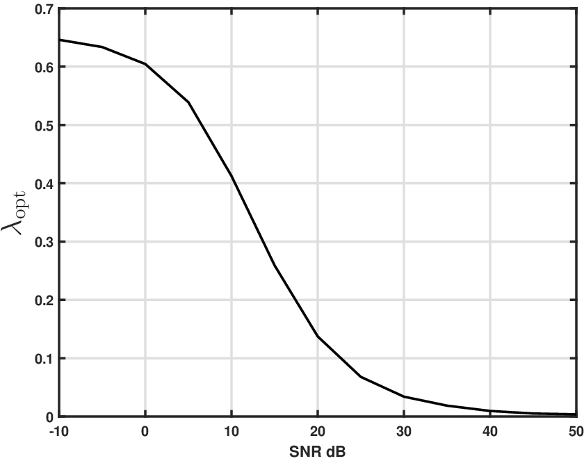
where $l_{j}\in\mathbb{C}$ is additive noise. The noise $l_{j}$ is assumed to be i.i.d. Gaussian with variance (average power) $\sigma_{\ell}^{2}$ and SNR (SNR) $\mathrm{SNR}=\frac{\|f\|_{L^{2}}^{2}}{\sigma_{\ell}^{2}(2n+1)}$ .

The sampling space consists of the exponential functions

u_{j}(x)=\e^{2\pi i\omega_{j}x}\chi_{[-\frac{1}{2},\frac{1}{2}]}(x),\quad j=-n,\dots,n\,,

so that indeed $d_{j}=\mathcal{F}f(\omega_{j})+l_{j}=\langle f,u_{j}\rangle_{L^{2}}+l_{j}$ .

The sampling frequencies $\omega_{j}\in\mathbb{R}$ are chosen

\omega_{j}=\frac{j}{2}+\delta_{j},\quad j=-n,\dots,n,

(45)

with $\delta_{j}\in[-2,2]$ i.i.d. and uniformly distributed over the interval $[-2,2]$ . The reconstruction space for the resampling problem is spanned by the complex exponentials

t_{k}(x)=\e^{2\pi ikx}\chi_{[-\frac{1}{2},\frac{1}{2}]}(x),\quad k=-m,\dots,m

with $m\leqslant n$ . In the numerical simulations we approximate the exponential function

f(x)=\e^{x}\chi_{[-\frac{1}{2},\frac{1}{2}]}(x),

from the noisy Fourier measurements (44). For the reconstruction we use the operators $Q_{\lambda}$ of Theorem 3.7. This means that the vector $\hat{c}=[\hat{c}_{-m},\dots,\hat{c}_{m}]^{T}$ containing the coefficients of the approximation

\tilde{f}=\sum_{k=-m}^{m}\hat{c}_{k}t_{k}(x)

of $f$ is the solution of the least squares problem

\hat{c}=\underset{c\in\ell^{2}(\mathbb{N})}{\textnormal{arg~min}}~\|\Sigma_{\lambda}^{-\frac{1}{2}}U^{*}Tc-\Sigma_{\lambda}^{-\frac{1}{2}}d\|_{2}^{2}.

(46)

For the particular bases $(u_{j}),(t_{k})$ consisting of exponentials, the cross-Gramian $U^{*}T\in\mathbb{C}^{(2n+1)\times(2m+1)}$ has the entries

(U^{*}T)(j,k)=\langle u_{j},t_{k}\rangle_{L^{2}}=\frac{\sin(\pi(\omega_{j}-k))}{\pi(\omega_{j}-k)}=\sinc(\omega_{j}-k),

and the preconditioning matrix $\Sigma_{\lambda}$ is given by the entries

\Sigma_{\lambda}(j,k)=\big(\lambda I_{2n+1}+(1-\lambda)G\big)(j,k)=\begin{cases}(1-\lambda)\sinc(\omega_{j}-\omega_{k})&\mbox{for }j\neq k,\\ 1&\mbox{for }j=k\,.\end{cases}

All results in this section have been averaged over $1000$ independent realizations of the sampling frequencies and the noise.

4.2. Noisy samples

In the first experiment we study the influence of the sampling rate $\frac{2m+1}{2n+1}$ and the SNR on the recovery performance of the operators $Q_{\lambda}$ . We approximate the exponential function $f(x)=\e^{x}\chi_{[-\frac{1}{2},\frac{1}{2}]}(x)$ from $181$ noisy Fourier samples ( $n=90$ ) and reconstruct in a space of trigonometric polynomials of degree $m=10,20,30,40$ (with dimension $2m+1$ ).

Table 1 lists the operator norm $\|Q_{\lambda}\|_{\rm op}$ , the quasi-optimality constant $\mu(Q_{\lambda})$ , the angle $\varphi_{\mathcal{T},\mathcal{U}}$ , the condition number $\kappa(\Sigma_{\lambda}^{-\frac{1}{2}}U^{*}T)$ of the matrix of the least squares problem (46) and the relative error $\frac{\|Q_{\lambda}h-f\|_{L^{2}}}{\|f\|_{L^{2}}}$ for $\text{SNR}=\infty$ , $\text{SNR}=20$ dB and $\text{SNR}=10$ dB and $m=10$ in (a), $m=20$ in (b) $m=30$ in (c) and $m=40$ in (d). All values are listed in the form $E\pm\sigma$ where $E$ is the expected value and $\sigma$ the standard deviation of the quantity, and rounded to the third decimal place.

	relative error $\frac{\\|Q_{\lambda}h-f\\|_{L^{2}}}{\\|f\\|_{L^{2}}}$
	$\text{SNR}\!=\!\infty$	$\text{SNR}\!=\!20$ dB	$\text{SNR}\!=\!10$ dB	$\\|Q_{\lambda}\\|_{\rm op}$	$\mu(Q_{\lambda})$	$\kappa(\Sigma_{\lambda}^{-\frac{1}{2}}U^{*}T)$
$Q_{0}$	$0.067\pm 0.000$	$0.088\pm 0.043$	$0.184\pm 0.165$	$8.288\pm 10.884$	$1.000\pm 0.000$	$1.000\pm 0.000$
$Q_{0.1}$	$0.068\pm 0.005$	$0.075\pm 0.011$	$0.118\pm 0.045$	$4.024\pm 3.907$	$1.078\pm 0.221$	$1.747\pm 1.233$
$Q_{0.2}$	$0.069\pm 0.010$	$0.076\pm 0.013$	$0.118\pm 0.045$	$3.936\pm 3.807$	$1.160\pm 0.382$	$2.256\pm 1.842$
$Q_{0.3}$	$0.071\pm 0.014$	$0.077\pm 0.016$	$0.118\pm 0.046$	$3.880\pm 3.744$	$1.245\pm 0.525$	$2.724\pm 2.369$
$Q_{0.4}$	$0.073\pm 0.019$	$0.079\pm 0.020$	$0.119\pm 0.048$	$3.838\pm 3.699$	$1.336\pm 0.662$	$3.190\pm 2.881$
$Q_{0.5}$	$0.076\pm 0.024$	$0.081\pm 0.024$	$0.120\pm 0.050$	$3.804\pm 3.662$	$1.434\pm 0.802$	$3.682\pm 3.412$
$Q_{0.6}$	$0.079\pm 0.028$	$0.084\pm 0.028$	$0.121\pm 0.053$	$3.776\pm 3.632$	$1.544\pm 0.950$	$4.224\pm 3.996$
$Q_{0.7}$	$0.082\pm 0.033$	$0.086\pm 0.033$	$0.123\pm 0.056$	$3.752\pm 3.608$	$1.670\pm 1.112$	$4.848\pm 4.672$
$Q_{0.8}$	$0.085\pm 0.039$	$0.089\pm 0.038$	$0.125\pm 0.060$	$3.733\pm 3.587$	$1.820\pm 1.298$	$5.603\pm 5.503$
$Q_{0.9}$	$0.089\pm 0.045$	$0.093\pm 0.044$	$0.127\pm 0.065$	$3.718\pm 3.572$	$2.011\pm 1.523$	$6.581\pm 6.616$
$Q_{1}$	$0.094\pm 0.052$	$0.098\pm 0.051$	$0.131\pm 0.071$	$3.712\pm 3.566$	$2.276\pm 1.824$	$7.982\pm 8.319$

(a)

m=10

\varphi_{\mathcal{T},\mathcal{U}}=1.7734e-08\pm 1.3455e-08

	relative error $\frac{\\|Q_{\lambda}h-f\\|_{L^{2}}}{\\|f\\|_{L^{2}}}$
	$\text{SNR}\!=\!\infty$	$\text{SNR}\!=\!20$ dB	$\text{SNR}\!=\!10$ dB	$\\|Q_{\lambda}\\|_{\rm op}$	$\mu(Q_{\lambda})$	$\kappa(\Sigma_{\lambda}^{-\frac{1}{2}}U^{*}T)$
$Q_{0}$	$0.048\pm 0.000$	$0.096\pm 0.060$	$0.259\pm 0.201$	$11.927\pm 12.724$	$1.000\pm 0.000$	$1.000\pm 0.000$
$Q_{0.1}$	$0.049\pm 0.003$	$0.066\pm 0.017$	$0.147\pm 0.056$	$5.330\pm 4.392$	$1.097\pm 0.201$	$2.103\pm 1.391$
$Q_{0.2}$	$0.050\pm 0.006$	$0.067\pm 0.018$	$0.146\pm 0.055$	$5.249\pm 4.320$	$1.194\pm 0.349$	$2.833\pm 2.088$
$Q_{0.3}$	$0.052\pm 0.009$	$0.068\pm 0.019$	$0.146\pm 0.055$	$5.199\pm 4.277$	$1.293\pm 0.480$	$3.499\pm 2.694$
$Q_{0.4}$	$0.054\pm 0.012$	$0.069\pm 0.021$	$0.146\pm 0.055$	$5.162\pm 4.245$	$1.398\pm 0.607$	$4.164\pm 3.286$
$Q_{0.5}$	$0.056\pm 0.015$	$0.070\pm 0.022$	$0.146\pm 0.056$	$5.133\pm 4.221$	$1.510\pm 0.735$	$4.867\pm 3.906$
$Q_{0.6}$	$0.058\pm 0.018$	$0.072\pm 0.024$	$0.147\pm 0.057$	$5.110\pm 4.201$	$1.634\pm 0.869$	$5.644\pm 4.591$
$Q_{0.7}$	$0.061\pm 0.021$	$0.074\pm 0.026$	$0.148\pm 0.057$	$5.090\pm 4.184$	$1.776\pm 1.014$	$6.546\pm 5.387$
$Q_{0.8}$	$0.064\pm 0.025$	$0.076\pm 0.029$	$0.148\pm 0.059$	$5.074\pm 4.171$	$1.945\pm 1.180$	$7.650\pm 6.372$
$Q_{0.9}$	$0.067\pm 0.028$	$0.079\pm 0.031$	$0.150\pm 0.060$	$5.062\pm 4.162$	$2.157\pm 1.378$	$9.102\pm 7.695$
$Q_{1}$	$0.071\pm 0.032$	$0.082\pm 0.035$	$0.151\pm 0.063$	$5.057\pm 4.158$	$2.451\pm 1.638$	$11.233\pm 9.726$

(b)

m=20

\varphi_{\mathcal{T},\mathcal{U}}=2.0805e-08\pm 1.2298e-08

	relative error $\frac{\\|Q_{\lambda}h-f\\|_{L^{2}}}{\\|f\\|_{L^{2}}}$
	$\text{SNR}\!=\!\infty$	$\text{SNR}\!=\!20$ dB	$\text{SNR}\!=\!10$ dB	$\\|Q_{\lambda}\\|_{\rm op}$	$\mu(Q_{\lambda})$	$\kappa(\Sigma_{\lambda}^{-\frac{1}{2}}U^{*}T)$
$Q_{0}$	$0.039\pm 0.000$	$0.122\pm 0.084$	$0.373\pm 0.292$	$17.371\pm 17.536$	$1.000\pm 0.000$	$1.000\pm 0.000$
$Q_{0.1}$	$0.040\pm 0.003$	$0.069\pm 0.021$	$0.180\pm 0.066$	$6.452\pm 4.861$	$1.129\pm 0.213$	$2.431\pm 1.552$
$Q_{0.2}$	$0.042\pm 0.006$	$0.069\pm 0.021$	$0.180\pm 0.066$	$6.369\pm 4.793$	$1.246\pm 0.373$	$3.348\pm 2.324$
$Q_{0.3}$	$0.044\pm 0.008$	$0.070\pm 0.022$	$0.178\pm 0.066$	$6.318\pm 4.752$	$1.363\pm 0.514$	$4.180\pm 2.998$
$Q_{0.4}$	$0.046\pm 0.011$	$0.071\pm 0.023$	$0.178\pm 0.066$	$6.282\pm 4.723$	$1.482\pm 0.649$	$5.008\pm 3.658$
$Q_{0.5}$	$0.048\pm 0.013$	$0.072\pm 0.023$	$0.178\pm 0.066$	$6.254\pm 4.701$	$1.610\pm 0.785$	$5.885\pm 4.350$
$Q_{0.6}$	$0.050\pm 0.015$	$0.073\pm 0.024$	$0.179\pm 0.066$	$6.232\pm 4.683$	$1.745\pm 0.928$	$6.856\pm 5.115$
$Q_{0.7}$	$0.052\pm 0.017$	$0.074\pm 0.025$	$0.179\pm 0.067$	$6.213\pm 4.667$	$1.900\pm 1.085$	$7.987\pm 6.007$
$Q_{0.8}$	$0.054\pm 0.020$	$0.075\pm 0.027$	$0.179\pm 0.068$	$6.198\pm 4.655$	$2.082\pm 1.265$	$9.378\pm 7.113$
$Q_{0.9}$	$0.056\pm 0.022$	$0.077\pm 0.028$	$0.180\pm 0.068$	$6.187\pm 4.646$	$2.310\pm 1.483$	$11.223\pm 8.600$
$Q_{1}$	$0.059\pm 0.024$	$0.079\pm 0.030$	$0.181\pm 0.069$	$6.183\pm 4.642$	$2.621\pm 1.775$	$13.966\pm 10.885$

(c)

m=30

\varphi_{\mathcal{T},\mathcal{U}}=3.5152e-08\pm 7.3768e-09

	relative error $\frac{\\|Q_{\lambda}h-f\\|_{L^{2}}}{\\|f\\|_{L^{2}}}$
	$\text{SNR}\!=\!\infty$	$\text{SNR}\!=\!20$ dB	$\text{SNR}\!=\!10$ dB	$\\|Q_{\lambda}\\|$	$\mu(Q_{\lambda})$	$\kappa(\Sigma_{\lambda}^{-\frac{1}{2}}U^{*}T)$
$Q_{0}$	$0.034\pm 0.000$	$0.870\pm 3.781$	$2.550\pm 9.917$	$180.730\pm 790.710$	$1.000\pm 1.000$	$1.000\pm 1.000$
$Q_{0.1}$	$0.036\pm 0.004$	$0.075\pm 0.025$	$0.209\pm 0.076$	$7.322\pm 5.272$	$1.185\pm 0.298$	$2.701\pm 1.705$
$Q_{0.2}$	$0.038\pm 0.007$	$0.075\pm 0.025$	$0.208\pm 0.073$	$7.229\pm 5.194$	$1.327\pm 0.469$	$3.758\pm 2.537$
$Q_{0.3}$	$0.040\pm 0.009$	$0.076\pm 0.026$	$0.207\pm 0.072$	$7.179\pm 5.153$	$1.456\pm 0.610$	$4.713\pm 3.263$
$Q_{0.4}$	$0.041\pm 0.011$	$0.076\pm 0.026$	$0.206\pm 0.072$	$7.146\pm 5.127$	$1.580\pm 0.739$	$5.667\pm 3.978$
$Q_{0.5}$	$0.043\pm 0.012$	$0.077\pm 0.027$	$0.206\pm 0.071$	$7.121\pm 5.107$	$1.707\pm 0.865$	$6.677\pm 4.729$
$Q_{0.6}$	$0.044\pm 0.014$	$0.077\pm 0.027$	$0.206\pm 0.071$	$7.102\pm 5.093$	$1.840\pm 0.993$	$7.800\pm 5.562$
$Q_{0.7}$	$0.046\pm 0.015$	$0.078\pm 0.028$	$0.206\pm 0.071$	$7.088\pm 5.081$	$1.983\pm 1.129$	$9.110\pm 6.535$
$Q_{0.8}$	$0.048\pm 0.017$	$0.079\pm 0.028$	$0.206\pm 0.071$	$7.076\pm 5.073$	$2.147\pm 1.281$	$10.729\pm 7.744$
$Q_{0.9}$	$0.049\pm 0.018$	$0.080\pm 0.029$	$0.206\pm 0.071$	$7.068\pm 5.067$	$2.344\pm 1.460$	$12.888\pm 9.374$
$Q_{1}$	$0.051\pm 0.019$	$0.081\pm 0.029$	$0.207\pm 0.072$	$7.065\pm 5.065$	$2.601\pm 1.689$	$16.127\pm 11.882$

(d)

m=40

\varphi_{\mathcal{T},\mathcal{U}}=5.4254e-08\pm 1.4382e-08

Table 1. Reconstruction of the exponential function by the operators

Q_{\lambda}

from noisy measurements

By (2) the (absolute) reconstruction error depends both on the quasi-optimality constant $\mu(Q_{\lambda})$ and the operator norm $\|Q_{\lambda}\|_{\rm op}$ . The numerical simulations support Theorem 3.5 asserting that the quasi-optimality constant $\mu$ is minimal for $\lambda=0$ . As expected in view of Lemma 3.8 the quasi-optimality constant $\mu$ is increasing with $\lambda$ . The angle $\varphi_{\mathcal{T},\mathcal{U}}$ is almost zero, so the reconstruction space is “almost contained” in the sampling space. Therefore $Q_{0}U^{*}$ is nearly identical to the orthogonal projection $P_{\mathcal{T}}$ onto $\mathcal{T}$ . A small angle $\varphi_{\mathcal{T},\mathcal{U}}$ is essential for stable reconstruction. Taking for example $m=n$ leads to an angle close to $\frac{\pi}{2}$ (since the sampling frequencies are contained in the interval $[-\frac{n}{2}-2,\frac{n}{2}+2]$ ), which necessarily leads to an unstable scenario. Taking more measurements than reconstruction vectors is a common way to stabilize the reconstruction problem [8, 7, 10, 6, 33, 27, 5, 24, 25, 26, 40, 1, 3, 2, 4, 11]. The operator norm of $Q_{\lambda}$ is decreasing in $\lambda$ , and the approximation becomes less sensitive to noise, with $Q_{1}$ being the most stable reconstruction in line with [9, Theorem 6.2.] and with Theorem 3.2. The intermediate reconstruction operators offer a trade-off between sensitivity to noise and the out-of-space contributions. A suitable choice of $\lambda$ then leads to more accurate reconstructions than $Q_{0}$ and $Q_{1}$ . For example for $m=10$ and $\acs{SNR}=20$ dB the average relative reconstruction error is $0.088$ for $Q_{0}$ , $0.098$ for $Q_{1}$ , but only $0.075$ for $Q_{0.1}$ .

Interestingly, for $\acs{SNR}=10$ dB we obtain a higher average approximation error for dimension $m=40$ than for $m=10,20,30$ . Although the increase in dimension makes the distance $\|f-P_{\mathcal{T}}f\|_{L^{2}}$ smaller, the high irregularity in the sampling frequencies seems to lead to unstable scenarios. This correlates nicely with the increase of the operator norm $\|Q_{\lambda}\|_{\rm op}$ with increasing $m$ .

We next observe that the condition number $\kappa(\Sigma_{\lambda}^{-\frac{1}{2}}U^{*}T)$ is increasing with $\lambda$ , as anticipated in Lemma 3.10. As discussed in Section 3.4, this opens the possibility of finding non-diagonal weight matrices.

For Figure 1(a) we have determined the parameter $\lambda_{\rm opt}$ such that the relative reconstruction error is minimal, i.e, $\lambda_{\rm opt}=\mathrm{arg~min}\frac{\|Q_{\lambda}d-f\|_{L^{2}}}{\|f\|_{L^{2}}}$ . We then plot the correlation between $\lambda_{\rm opt}$ and the signal-to-noise ratio. The plot confirms Theorems 3.5 and 3.2: for $\mathrm{SNR}\to\infty$ the optimal reconstruction is with $Q_{0}$ , and for $\mathrm{SNR}\to-\infty$ , the optimal reconstruction is with $Q_{1}$ .

In Figure 1(b) we depict the approximations obtained by $Q_{0}$ , $Q_{1}$ and $Q_{\lambda_{\rm{opt}}}$ for a single realization of the sampling frequencies and noise with $m=20$ and SNR $=20$ dB. The optimal choice of the regularization parameter $\lambda_{\rm{opt}}$ yields a significantly better approximation than the standard least square approximation (with $Q_{1}$ ).

In Figure 1(c) we depict the quasi-optimality constant $\mu(Q_{\lambda})$ versus the operator norm $\|Q_{\lambda}\|_{\rm op}$ for $\lambda\in[0,1]$ for $m=20$ and SNR $=20$ dB. The curve consists of the points $(\mu(Q_{\lambda}),\|Q_{\lambda}\|_{\rm op})$ for $\lambda\in[0,1]$ . This curve exhibits a striking change of direction at a small value of $\lambda$ , as is shown by the points corresponding to $\lambda=10^{-6},0.01,0.1$ . The value of $\lambda$ near the edge of the curve (around $0.01$ ) yields a good trade-off between quasi-optimality and operator norm.

Figure 1(d) shows the relative reconstruction error $\frac{\|Q_{\lambda}d-f\|_{L^{2}}}{\|f\|_{L^{2}}}$ as a function of $\lambda$ for fixed $\mathrm{SNR}$ . This is a typical $L$ -curve known from many regularization procedures of ill-posed problems. The plots supports the interpretation of $\lambda$ as a regularization parameter.

Refer to caption — (a) The SNR versus $\lambda_{\rm{opt}}$ .

4.3. Reconstruction from measurements of a biased function

We now assume that we are given a set of Fourier measurements of a perturbation of $f\in\mathcal{H}$

\tilde{d}=[\mathcal{F}(f+\Delta f)(\omega_{-n}),\dots,\mathcal{F}(f+\Delta f)(\omega_{n})]^{T}.

The sampling frequencies $\omega_{j}$ are as in (45) with $\delta_{j}\in[-2,2]$ . For each set of sampling frequencies we choose $\Delta f$ as a trigonometric polynomial

\Delta f=\sum_{j=-\frac{n}{2}}^{\frac{n}{2}}a_{j}\e^{2i\pi j\cdot}\chi_{[-1/2,1/2]}.

(47)

The coefficients $a_{j}$ in (47) are i.i.d. Gaussian distributed with variance (average power) $\sigma^{2}$ . Table 2 shows the relative error $\frac{\|Q_{\lambda}\tilde{d}-f\|_{L^{2}}}{\|f\|_{L^{2}}}$ for $\text{SNR}=\infty$ , $\text{SNR}=20$ dB and $\text{SNR}=10$ dB and $m=10$ in (a), $m=20$ in (b), $m=30$ in (c) and $m=40$ in (d). In this case the most accurate reconstruction is always given by the reconstruction with the operator $Q_{0}$ , thus confirming Corollary 3.14. In addition, with increasing dimension of the reconstruction space the distance $\|f-P_{\mathcal{T}}f\|_{L^{2}}$ is decreasing with $m$ , and the relative error decreases up to $m=40$ . For $m=50$ the angle between the sampling and reconstruction space is $\varphi_{\mathcal{T},\mathcal{U}}=0.309\pm 0.094$ , which results in a significantly higher approximation error.

	relative error $\frac{\\|Q_{\lambda}h-f\\|_{L^{2}}}{\\|f\\|_{L^{2}}}$
	$\text{SNR}\!=\!\infty$	$\text{SNR}\!=\!20$ dB	$\text{SNR}\!=\!10$ dB
$Q_{0}$	$0.067\pm 0.000$	$0.075\pm 0.003$	$0.127\pm 0.020$
$Q_{0.1}$	$0.068\pm 0.003$	$0.076\pm 0.004$	$0.128\pm 0.020$
$Q_{0.2}$	$0.069\pm 0.007$	$0.077\pm 0.007$	$0.129\pm 0.021$
$Q_{0.3}$	$0.071\pm 0.011$	$0.079\pm 0.011$	$0.131\pm 0.022$
$Q_{0.4}$	$0.073\pm 0.015$	$0.081\pm 0.015$	$0.132\pm 0.024$
$Q_{0.5}$	$0.075\pm 0.019$	$0.083\pm 0.018$	$0.134\pm 0.027$
$Q_{0.6}$	$0.078\pm 0.023$	$0.086\pm 0.022$	$0.136\pm 0.030$
$Q_{0.7}$	$0.081\pm 0.027$	$0.088\pm 0.027$	$0.139\pm 0.034$
$Q_{0.8}$	$0.084\pm 0.032$	$0.092\pm 0.031$	$0.142\pm 0.038$
$Q_{0.9}$	$0.088\pm 0.037$	$0.095\pm 0.037$	$0.146\pm 0.044$
$Q_{1}$	$0.093\pm 0.043$	$0.100\pm 0.043$	$0.151\pm 0.051$

(a)

m=10

	relative error $\frac{\\|Q_{\lambda}h-f\\|_{L^{2}}}{\\|f\\|_{L^{2}}}$
	$\text{SNR}\!=\!\infty$	$\text{SNR}\!=\!20$ dB	$\text{SNR}\!=\!10$ dB
$Q_{0}$	$0.048\pm 0.000$	$0.067\pm 0.005$	$0.159\pm 0.023$
$Q_{0.1}$	$0.049\pm 0.002$	$0.068\pm 0.006$	$0.160\pm 0.022$
$Q_{0.2}$	$0.050\pm 0.005$	$0.069\pm 0.007$	$0.161\pm 0.023$
$Q_{0.3}$	$0.052\pm 0.008$	$0.071\pm 0.009$	$0.162\pm 0.023$
$Q_{0.4}$	$0.054\pm 0.011$	$0.073\pm 0.011$	$0.163\pm 0.024$
$Q_{0.5}$	$0.056\pm 0.014$	$0.074\pm 0.013$	$0.164\pm 0.025$
$Q_{0.6}$	$0.059\pm 0.017$	$0.076\pm 0.016$	$0.166\pm 0.027$
$Q_{0.7}$	$0.061\pm 0.020$	$0.079\pm 0.019$	$0.168\pm 0.029$
$Q_{0.8}$	$0.064\pm 0.023$	$0.081\pm 0.022$	$0.170\pm 0.032$
$Q_{0.9}$	$0.067\pm 0.026$	$0.084\pm 0.026$	$0.173\pm 0.037$
$Q_{1}$	$0.071\pm 0.030$	$0.088\pm 0.030$	$0.176\pm 0.043$

(b)

m=20

	relative error $\frac{\\|Q_{\lambda}h-f\\|_{L^{2}}}{\\|f\\|_{L^{2}}}$
	$\text{SNR}\!=\!\infty$	$\text{SNR}\!=\!20$ dB	$\text{SNR}\!=\!10$ dB
$Q_{0}$	$0.039\pm 0.000$	$0.070\pm 0.006$	$0.189\pm 0.023$
$Q_{0.1}$	$0.041\pm 0.003$	$0.071\pm 0.007$	$0.189\pm 0.023$
$Q_{0.2}$	$0.042\pm 0.006$	$0.072\pm 0.008$	$0.190\pm 0.023$
$Q_{0.3}$	$0.044\pm 0.008$	$0.073\pm 0.009$	$0.191\pm 0.023$
$Q_{0.4}$	$0.046\pm 0.011$	$0.075\pm 0.010$	$0.192\pm 0.024$
$Q_{0.5}$	$0.048\pm 0.013$	$0.076\pm 0.012$	$0.193\pm 0.024$
$Q_{0.6}$	$0.050\pm 0.015$	$0.078\pm 0.014$	$0.194\pm 0.025$
$Q_{0.7}$	$0.052\pm 0.017$	$0.079\pm 0.016$	$0.195\pm 0.026$
$Q_{0.8}$	$0.055\pm 0.020$	$0.081\pm 0.018$	$0.197\pm 0.027$
$Q_{0.9}$	$0.057\pm 0.022$	$0.083\pm 0.020$	$0.199\pm 0.029$
$Q_{1}$	$0.060\pm 0.025$	$0.086\pm 0.023$	$0.202\pm 0.033$

(c)

m=30

	relative error $\frac{\\|Q_{\lambda}h-f\\|_{L^{2}}}{\\|f\\|_{L^{2}}}$
	$\text{SNR}\!=\!\infty$	$\text{SNR}\!=\!20$ dB	$\text{SNR}\!=\!10$ dB
$Q_{0}$	$0.034\pm 0.000$	$0.075\pm 0.007$	$0.215\pm 0.023$
$Q_{0.1}$	$0.036\pm 0.003$	$0.076\pm 0.007$	$0.216\pm 0.023$
$Q_{0.2}$	$0.038\pm 0.006$	$0.077\pm 0.008$	$0.217\pm 0.023$
$Q_{0.3}$	$0.040\pm 0.008$	$0.078\pm 0.008$	$0.218\pm 0.023$
$Q_{0.4}$	$0.041\pm 0.010$	$0.079\pm 0.009$	$0.218\pm 0.023$
$Q_{0.5}$	$0.043\pm 0.011$	$0.080\pm 0.010$	$0.219\pm 0.024$
$Q_{0.6}$	$0.045\pm 0.013$	$0.082\pm 0.011$	$0.220\pm 0.024$
$Q_{0.7}$	$0.046\pm 0.014$	$0.083\pm 0.013$	$0.221\pm 0.025$
$Q_{0.8}$	$0.048\pm 0.016$	$0.084\pm 0.014$	$0.222\pm 0.026$
$Q_{0.9}$	$0.050\pm 0.017$	$0.085\pm 0.015$	$0.223\pm 0.027$
$Q_{1}$	$0.051\pm 0.019$	$0.087\pm 0.016$	$0.225\pm 0.029$

(d)

m=40

Table 2. Reconstruction of the exponential function by the operators

Q_{\lambda}

from measurements of the biased function

APPENDIX: FRAMES IN HILBERT SPACES

We need the definition of the Moore-Penrose pseudoinverse of an operator on a Hilbert space [15, Section 2.5]. We use the notation $\mathcal{R}(A)$ for the range, and $\mathcal{N}(A)$ for the null-space of the operator $A$ .

Definition 4.1.

Let $\mathcal{H}$ and $\mathcal{W}$ be Hilbert spaces. If $A:\mathcal{W}\rightarrow\mathcal{H}$ is a bounded operator with a closed range $\mathcal{R}(A)$ , then there exists a unique bounded operator $A^{\dagger}:\mathcal{H}\rightarrow\mathcal{W}$ satisfying

		$\displaystyle\mathcal{N}(A^{\dagger})=\mathcal{R}(A)^{\perp}=\mathcal{N}(A^{*}),$
		$\displaystyle\mathcal{R}(A^{\dagger})=\mathcal{N}(A)^{\perp}=\mathcal{R}(A^{*}),\text{ and }$
		$\displaystyle AA^{\dagger}x=x,~x\in\mathcal{R}(A).$

The operator $A^{\dagger}$ is called the Moore-Penrose pseudoinverse of $A$ .

For a sequence $(u_{j})_{j\in\mathbb{N}}$ we define the synthesis operator on the subspace of finite sequences by

U(c_{j})_{j\in\mathbb{N}}=\sum_{j=1}^{\infty}c_{j}u_{j}\,.

Definition 4.2.

(i) If $U$ can be extended to a bounded operator $U:\ell^{2}(\mathbb{N})\rightarrow\mathcal{H}$ , $(u_{j})_{j\in\mathbb{N}}$ is called a Bessel sequence.

(ii) If $U$ is bounded $U:\ell^{2}(\mathbb{N})\rightarrow\mathcal{H}$ , $(u_{j})_{j\in\mathbb{N}}$ and has closed range, $(u_{j})_{j\in\mathbb{N}}$ is called a frame for the subspace $\mathcal{U}=\overline{\textnormal{span}}(u_{j})_{j\in\mathbb{N}}$ .

(iii) If $(u_{j})_{j\in\mathbb{N}}$ is a Bessel sequence, then the adjoint operator of $U$ is the analysis operator

U^{*}:\mathcal{H}\rightarrow\ell^{2}(\mathbb{N}),\quad U^{*}f=(\langle f,u_{j}\rangle_{\mathcal{H}})_{j\in\mathbb{N}}\,,

and $S=UU^{*}:\mathcal{H}\to\mathcal{H}$ , $Sf=\sum_{j=1}^{\infty}\langle f,u_{j}\rangle_{\mathcal{H}}u_{j}$ is the frame operator of $(u_{j})$ .

(iv) The sequence $(S^{\dagger}u_{j})_{j\in\mathbb{N}}\subseteq\mathcal{U}$ is the canonical dual frame in $\mathcal{U}$ , and every $f\in\mathcal{U}$ possesses the frame expansions

f=\sum_{j\in\mathbb{N}}\langle f,S^{\dagger}u_{j}\rangle_{\mathcal{H}}u_{j}=\sum_{j\in\mathbb{N}}\langle f,u_{j}\rangle_{\mathcal{H}}S^{\dagger}u_{j}

with unconditional convergence of both series.

Lemma 4.3.

Let $\mathcal{U}$ be a closed subspace of $\mathcal{H}$ and let $(u_{j})_{j\in\mathbb{N}}$ be a frame for $\mathcal{U}$ .The set

(S^{\frac{\dagger}{2}}u_{j})_{j\in\mathbb{N}}

forms a tight frame for $\mathcal{U}$ with frame bound equal to $1$ . The synthesis operator $M$ of the sequence $(S^{\frac{\dagger}{2}}u_{j})_{j\in\mathbb{N}}$ is given by $M:=S^{\frac{\dagger}{2}}U$ , and

P_{\mathcal{U}}=MM^{*}=S^{\frac{\dagger}{2}}SS^{\frac{\dagger}{2}}=S^{\dagger}S=SS^{\dagger}.

Lemma 4.4 proves the following. Suppose that we are given the inner products $(\langle f,u_{j}\rangle_{\mathcal{H}})_{j\in\mathbb{N}}$ of an element $f\in\mathcal{H}$ with a frame $(u_{j})_{j\in\mathbb{N}}$ for $\mathcal{U}$ (a closed subspace of $\mathcal{H}$ ). Applying the operator $(U^{*}U)^{\frac{\dagger}{2}}$ to these measurements, we obtain the inner products of $f$ with the tight frame $(S^{\frac{\dagger}{2}}u_{j})_{j\in\mathbb{N}}$ for $\mathcal{U}$ .

Lemma 4.4.

Let $\mathcal{U}$ be a closed subspace of $\mathcal{H}$ and $(u_{j})_{j\in\mathbb{N}}$ a frame for $\mathcal{U}$ with synthesis operator $U$ , analysis operator $U^{*}$ , Gramian $G=U^{*}U$ and frame operator $S=UU^{*}$ . Then

G^{\frac{\dagger}{2}}U^{*}=U^{*}S^{\frac{\dagger}{2}}.

Thus, $G^{\frac{\dagger}{2}}U^{*}$ is the analysis operator of the tight frame sequence $(S^{\frac{\dagger}{2}}u_{j})_{j\in\mathbb{N}}$ .

Proof.

Obviously for $k\in\mathbb{N}$

(U^{*}U)^{k}U^{*}=U^{*}(UU^{*})^{k}.

Therefore,

p(G)U^{*}=U^{*}p(S)

for every polynomial $p$ . We are going to prove that there exists a sequence of polynomials $(p_{k})_{k\in\mathbb{N}}$ , such that for $i=1,2$

\underset{m\rightarrow\infty}{\lim}\|p_{m}(M_{i})-M_{i}^{\frac{\dagger}{2}}\|_{\rm op}=0

simultaneously for $M_{1}:=G$ and $M_{2}:=S$ .

Let $A$ and $B$ denote the lower bound and upper frame bound of the frame sequence $(u_{j})_{j\in\mathbb{N}}$ . From the lower frame bound $A$ we infer that for every $f\in\mathcal{U}=\mathcal{N}(UU^{*})^{\perp}=\mathcal{N}(S)^{\perp}$

A\|f\|_{\mathcal{H}}^{2}\leqslant\langle Sf,f\rangle_{\mathcal{H}}.

Consequently the set $\sigma(S)\backslash\{0\}$ is bounded below by $A$ . Here $\sigma(S)$ denotes the spectrum of the operator $S$ . The upper frame bound $B$ ensures that the set $\sigma(S)$ has the upper bound $B$ . This shows that $0$ is an isolated point of the spectrum, and that for ${K:=\{0\}\cup[A,B]}$ the function ${h:K\rightarrow\mathbb{R}}$

\displaystyle\ h(x)=\begin{cases}\frac{1}{\sqrt{x}}&\text{for }x\in[A,B],\\ 0&\text{for }x=0\end{cases}

is continuous on $K$ . Since $\sigma(S)\cup\{0\}=\sigma(G)\cup\{0\}$ , $h$ is also continuous on $\sigma(G)$ .

By the Weierstrass approximation theorem there exists a sequence of polynomials $(p_{m})_{m\in\mathbb{N}}$ , such that

\underset{m\rightarrow\infty}{\lim}\|p_{m}-h\|_{\infty}=0,

uniformly on $K$ . By the continuous functional calculus

\underset{m\rightarrow\infty}{\lim}\|p_{m}(M_{i})-h(M_{i})\|_{\rm op}=0

simultaneously for $M_{1}:=G$ and $M_{2}:=S$ and $h(M_{i})=M_{i}^{\frac{\dagger}{2}}$ for $i=1,2$ . ∎

Lemma 4.5.

[15, Lemma 5.3.6] Let $(f_{j})_{j\in\mathbb{N}}$ be a frame for $\mathcal{H}$ with frame operator $S$ and let $f\in\mathcal{H}$ . If $f$ has a representation $f=\sum_{j\in\mathbb{N}}c_{j}f_{j}$ for some coefficients $(c_{j})_{j\in\mathbb{N}}$ , then

\sum_{j\in\mathbb{N}}|c_{j}|^{2}=\sum_{j\in\mathbb{N}}|\langle f,S^{-1}f_{j}\rangle_{\mathcal{H}}|^{2}+\sum_{j\in\mathbb{N}}|c_{j}-\langle f,S^{-1}f_{j}\rangle_{\mathcal{H}}|^{2}.

References

[1] B. Adcock, M. Gataric, and A. Hansen. On stable reconstructions from nonuniform Fourier measurements. SIAM J. Imaging Sci., 7(3):1690–1723, 2014.
[2] B. Adcock, M. Gataric, and A. C. Hansen. Recovering Piecewise Smooth Functions from Nonuniform Fourier Measurements, Spectral and High Order Methods for Partial Differential Equations ICOSAHOM, volume 106 of Lecture Notes in Computational Science and Engineering, 117–125, 2015.
[3] B. Adcock, M. Gataric, and A. C. Hansen. Weighted frames of exponentials and stable recovery of multidimensional functions from nonuniform Fourier samples. Appl. Comput. Harmon. Anal., 42(3):508–535, 2017.
[4] B. Adcock, M. Gataric, and A. C. Hansen. Density theorems for nonuniform sampling of bandlimited functions using derivatives or bunched measurements. J. Fourier Anal. Appl., pages 1–37, 2016.
[5] B. Adcock, M. Gataric, and J. L. Romero. Data assimilation in Banach spaces. arXiv preprint arXiv:1606.07698, 2017.
[6] B. Adcock and A. C. Hansen. A generalized sampling theorem for stable reconstructions in arbitrary bases. J. Fourier Anal. Appl., 18(4):685–716, 2012.
[7] B. Adcock and A. C. Hansen. Stable reconstructions in Hilbert spaces and the resolution of the Gibbs phenomenon. Appl. Comput. Harmon. Anal., 32(3):357–388, 2012.
[8] B. Adcock, A. C. Hansen, G. Kutyniok, and M. Gitta. Linear stable sampling rate: optimality of 2D wavelet reconstructions from Fourier measurements. SIAM J. Math. Anal., 47(2):1196–1233, 2015.
[9] B. Adcock, A. C. Hansen, and C. Poon. Beyond consistent reconstructions: optimality and sharp bounds for generalized sampling, and application to the uniform resampling problem. SIAM J. Math. Anal., 45(5):3132–3167, 2013.
[10] B. Adcock, A. C. Hansen, and C. Poon. On optimal wavelet reconstructions from Fourier samples: linearity and universality of the stable sampling rate. Appl. Comput. Harmon. Anal., 36(3):387–415, 2014.
[11] A. Aldroubi and K. Gröchenig. Nonuniform sampling and reconstruction in shift-invariant spaces. SIAM Rev., 43(4):585–620, 2001.
[12] J. Antezana and G. Corach. Sampling theory, oblique projections and a question by Smale and Zhou. Appl. Comput. Harmon. Anal., 21(2):245–253, 2006.
[13] P. Binev, A. Cohen, W. Dahmen, R. DeVore, G. Petrova, and P. Wojtaszczyk. Data assimilation in reduced modeling. SIAM/ASA Journal on Uncertainty Quantification, 5(1):1–29, 2017.
[14] D. Buckholtz. Hilbert space idempotents and involutions. Proc. Amer. Math. Soc., 128(5):1415–1418, 2000.
[15] O. Christensen. Frames and bases. Applied and Numerical Harmonic Analysis. Birkhäuser Boston, Inc., Boston, MA, 2008. An introductory course.
[16] O. Christensen and Y. C. Eldar. Oblique dual frames and shift-invariant spaces. Appl. Comput. Harmon. Anal., 17(1):48–68, 2004.
[17] O. Christensen and Y. C. Eldar. Generalized shift-invariant systems and frames for subspaces. J. Fourier Anal. Appl., 11(3):299–313, 2005.
[18] R. DeVore, G. Petrova, and P. Wojtaszczyk. Data assimilation in Banach spaces. arXiv preprint arXiv:1602.06342, 2016.
[19] Y. C. Eldar. Sampling with arbitrary sampling and reconstruction spaces and oblique dual frame vectors. J. Fourier Anal. Appl., 9(1):77–96, 2003.
[20] Y. C. Eldar. Sampling without input constraints: consistent reconstruction in arbitrary spaces. In Sampling, wavelets, and tomography, Appl. Numer. Harmon. Anal., pages 33–60. Birkhäuser Boston, Boston, MA, 2004.
[21] Y. C. Eldar and O. Christensen. Characterization of oblique dual frame pairs. EURASIP J. Appl. Signal Process., (Frames and overcomplete representations in signal processing, communications, and information theory):Art. ID 92674, 11, 2006.
[22] Y. C. Eldar and T. Werther. General framework for consistent sampling in Hilbert spaces. Int. J. Wavelets Multiresolut. Inf. Process., 3(3):347–359, 2005.
[23] H. G. Feichtinger, and K. Gröchenig. Theory and practice of irregular sampling. In Wavelets: mathematics and applications, Stud. Adv. Math., pages 305–363. CRC, Boca Raton, FL, 1994.
[24] H. G. Feichtinger, K. Gröchenig, and T. Strohmer. Efficient numerical methods in non-uniform sampling theory. Numer. Math., 69(4):423–440, 1995.
[25] K. Gröchenig. Irregular sampling, Toeplitz matrices, and the approximation of entire functions of exponential type. Math. Comp., 68(226):749–765, 1999.
[26] K. Gröchenig. Non-uniform sampling in higher dimensions: from trigonometric polynomials to bandlimited functions. In Modern sampling theory, Appl. Numer. Harmon. Anal., pages 155–171. Birkhäuser Boston, Boston, MA, 2001.
[27] T. Hrycak and K. Gröchenig. Pseudospectral Fourier reconstruction with the modified inverse polynomial reconstruction method. J. Comput. Phys., 229(3):933–946, 2010.
[28] J.-H. Jung and B. D. Shizgal. Generalization of the inverse polynomial reconstruction method in the resolution of the Gibbs phenomenon. J. Comput. Appl. Math., 172(1):131–151, 2004.
[29] J.-H. Jung and B. D. Shizgal. Inverse polynomial reconstruction of two dimensional Fourier images. J. Sci. Comput., 25(3):367–399, 2005.
[30] J.-H. Jung and B. D. Shizgal. On the numerical convergence with the inverse polynomial reconstruction method for the resolution of the Gibbs phenomenon. J. Comput. Phys., 224(2):477–488, 2007.
[31] R. Lewitt. Reconstruction algorithms: Transform methods. Proceedings of the IEEE, 71(3):390–408, 1983.
[32] S. Li and H. Ogawa. Pseudoframes for subspaces with applications. J. Fourier Anal. Appl., 10(4):409–431, 2004.
[33] J. Ma. Generalized sampling reconstruction from Fourier measurements using compactly supported shearlets. Appl. Comput. Harmon. Anal., 42(2):294–318, 2017.
[34] Y. Maday and O. Mula. A generalized empirical interpolation method: application of reduced basis techniques to data assimilation. In Analysis and numerics of partial differential equations, volume 4 of Springer INdAM Ser., pages 221–235. Springer, Milan, 2013.
[35] Y. Maday, O. Mula, A. T. Patera, and M. Yano. The generalized empirical interpolation method: stability theory on Hilbert spaces with an application to the Stokes equation. Comput. Methods Appl. Mech. Engrg., 287:310–334, 2015.
[36] Y. Maday, A. T. Patera, J. D. Penn, and M. Yano. A parameterized-background data-weak approach to variational data assimilation: formulation, analysis, and application to acoustics. Internat. J. Numer. Methods Engrg., 102(5):933–965, 2015.
[37] C. C. Paige and M. A. Saunders. LSQR: an algorithm for sparse linear equations and sparse least squares. ACM Trans. Math. Software, 8(1):43–71, 1982.
[38] B. D. Shizgal and J.-H. Jung. Towards the resolution of the Gibbs phenomena. J. Comput. Appl. Math., 161(1):41–65, 2003.
[39] J. Steinberg. Oblique projections in Hilbert spaces. Integral Equations Operator Theory, 38(1):81–119, 2000.
[40] T. Strohmer. Numerical analysis of the non-uniform sampling problem. J. Comput. Appl. Math., 122(1-2):297–316, 2000.
[41] D. B. Szyld. The many proofs of an identity on the norm of oblique projections. Numer. Algorithms, 42(3-4):309–323, 2006.
[42] W.-S. Tang. Oblique projections, biorthogonal Riesz bases and multiwavelets in Hilbert spaces. Proc. Amer. Math. Soc., 128(2):463–473, 2000.
[43] A. Viswanathan, A. Gelb, D. Cochran, and R. Renaut. On reconstruction from non-uniform spectral data. J. Sci. Comput., 45(1-3):487–513, 2010.

Sampling and Reconstruction in Distinct Subspaces Using Oblique ProjectionsThanks: Funding by the Austrian Science Fund (FWF) through grant NFN SISE (S10602) and P26273 - N25 and by the Vienna Science and Technology Fund (WWTF) through project VRG12-009 and project ICT15-119.

Abstract.

1. Introduction

1.1. The reconstruction problem

1.2. Areas of application and related work

1.3. The reconstruction operators

1.4. Contributions

2. Classification of all reconstruction operators

Definition 2.1.

Theorem 2.2.

Definition 2.3.

Lemma 2.4.

Corollary 2.5.

Lemma 2.6.

Proof.

3. The reconstruction operators

3.1. Least squares and the operator Q1Q_{1}

Theorem 3.1.

Proof.

Theorem 3.2.

Proof.

3.2. The operator Q0Q_{0}

Theorem 3.3.

Proof.

Remark 3.4.

Theorem 3.5.

Proof.

3.3. Combinations of Q0Q_{0} and Q1Q_{1}

Lemma 3.6.

Proof.

Theorem 3.7.

Proof.

Lemma 3.8.

Proof.

Remark 3.9.

3.4. Numerical calculation of the coefficients

Lemma 3.10.

Proof.

Remark 3.11.

3.5. Conditions for the approximations to coincide

Lemma 3.12.

Proof.

Theorem 3.13.

Proof.

3.6. Stability with respect to a biased objects

Corollary 3.14.

4. Numerical experiments for reconstruction from Fourier measurements

4.1. Setup

4.2. Noisy samples

4.3. Reconstruction from measurements of a biased function

APPENDIX: FRAMES IN HILBERT SPACES

Definition 4.1.

Definition 4.2.

Lemma 4.3.

Lemma 4.4.

Proof.

Lemma 4.5.

References

3.1. Least squares and the operator $Q_{1}$

3.2. The operator $Q_{0}$

3.3. Combinations of $Q_{0}$ and $Q_{1}$