CERN-TH-2017-132
High-Precision Calculations in Strongly Coupled Quantum Field Theory
with Next-to-Leading-Order Renormalized Hamiltonian Truncation
Abstract
Hamiltonian Truncation (a.k.a. Truncated Spectrum Approach) is an efficient numerical technique to solve strongly coupled QFTs in spacetime dimensions. Further theoretical developments are needed to increase its accuracy and the range of applicability. With this goal in mind, here we present a new variant of Hamiltonian Truncation which exhibits smaller dependence on the UV cutoff than other existing implementations, and yields more accurate spectra. The key idea for achieving this consists in integrating out exactly a certain class of high energy states, which corresponds to performing renormalization at the cubic order in the interaction strength. We test the new method on the strongly coupled two-dimensional quartic scalar theory. Our work will also be useful for the future goal of extending Hamiltonian Truncation to higher dimensions .
Introduction. Many interesting strongly interacting Quantum Field Theories (QFTs) are not amenable to analytical treatment. Such theories are often studied via Lattice Monte Carlo (LMC) numerical simulations, starting from the discretized Euclidean action. However, LMC has some drawbacks, for example it cannot easily compute real-time observables, it is rather computationally expensive, and it cannot directly describe renormalization group (RG) flows starting from interacting fixed points. Therefore, it is worth exploring other numerical approaches to strongly interacting QFTs. One promising alternative is provided by the Hamiltonian methods, which look for the eigenstates of the quantum Hamiltonian. These methods use various finite-dimensional approximations to the full infinite-dimensional QFT Hilbert space. Notable examples are the methods using Matrix Product States [1, 2] and more general Tensor Networks [3] such as MERA [4] or PEPS [5]. In this paper we will be concerned with another representative of this group of methods—Hamiltonian Truncation (HT), also known as the Truncated Spectrum (or Space) Approach, which is a direct generalization of the variational Rayleigh-Ritz (RR) method from quantum mechanics. This method goes back to the seminal work of Yurov and Al. Zamolodchikov [6, 7] and has since been applied in many contexts. See [8] for a recent extensive review and the bibliography.
The idea of HT is simple. The QFT Hamiltonian operator is split as where is an exactly solvable Hamiltonian whose eigenstates form the basis of the Hilbert space. One quantizes at surfaces of constant time and works in finite volume so that the spectrum is discrete 11 1 In relativistic QFTs one can also quantize on surfaces of constant light-cone coordinate. This light front quantization [39] is also used in numerical solutions of strongly coupled QFTs via a version of HT; some recent work is [40, 41, 42, 43, 44, 45]. The structure of the unperturbed Hilbert space is different from the equal time case, which leads to important differences in the numerical procedure. All technical claims in this work will refer exclusively to the equal time quantization.. The Hilbert space is then truncated to the low-lying eigenvectors of . The matrix of in this truncated Hilbert space is diagonalized exactly on a computer, to find the low-energy spectrum of interacting eigenstates.
As was understood early on [10], the numerical convergence of the HT depends crucially on the scaling dimension of the interaction . If the interaction is strongly relevant, in the RG sense, then HT converges fast, but convergence rate worsens as increases. This is a limitation of the method. For interaction dimensions larger that , naive HT actually diverges [10]. To ensure the convergence, we will assume here that
| (1) |
Another limitation of HT, as of many variational methods in general, is that the Hilbert space grows exponentially with the cutoff. Specifically, the dimension grows as , where is a theory-dependent constant and is the energy cutoff on the spectrum. The exponent typically depends on the spacetime dimension as , so this problem becomes more severe in higher . These two limitations are the main reason why the HT has been so far applied mainly in .
Motivated by the need to mitigate the above limitations, the recent works [11, 12, 13, 14] (following notably [15]; see also [16, 17, 18]) started developing the theory of renormalized HT, in which high-energy modes are not simply truncated away, but integrated out to produce an effective low energy Hamiltonian. As a result the convergence is improved. Renormalized HT has been applied in several strongly coupled QFT studies in [15, 18, 12, 13, 14] and in one study in [11]. We hope that in the future Hamiltonian Truncation will develop into an accurate numerical method, applicable also in . Here we will take another step towards this goal by proposing a novel and still more accurate approach to renormalization. A more detailed technical account of our work will appear elsewhere [19].
Setup. Consider the Hamiltonian of a QFT in finite volume, which we assume can be split into a solvable part , whose eigenfunction and eigenvectors are known, plus an interaction , whose matrix elements are computable in the basis of eigenstates of :
| (2) |
The can represent a free or an integrable Hamiltonian, or the Hamiltonian of a conformal field theory (CFT) on the cylinder . We assume that its finite volume spectrum is discrete, which is the case for most ’s of interest. Notice that although numerical HT calculations are performed in finite volume, infinite volume observables can then be extracted via controlled extrapolation.
The spectrum of the interacting theory is found by solving the eigenvalue equation:
| (3) |
where is the energy of a given state, and the corresponding eigenvector living in the Hilbert space spanned by the eigenstates of . Eq. (3) is infinite-dimensional and cannot be solved on a computer. So we split into a finite-dimensional “low-energy” part and a “high-energy” part . Motivated by effective field theory, a natural choice is to include into all the states with energy below a given cutoff , which plays the role of a UV cutoff. This should provide a good approximation for the interacting eigenstates with energy well below the cutoff. Different types of cutoff are possible but will not be considered here. We then project the eigenvalue equation onto those subspaces:
| (4) | ||||
| (5) |
where is the low/high energy split of , i.e. , , where , are the projectors on , . Similarly, , and so on.
The raw HT consists in throwing out all the states in and solving the eigenvalue equation,
| (6) |
By the min-max theorem, as the cutoff is increased, the eigenvalues approach the exact eigenvalues from above. As shown in [11], the raw HT numerical spectrum is expected to converge with polynomial rate , with by our assumption (1). This polynomial convergence must compete with the exponential growth of states in the Hilbert space.
It is possible to do better than in (6). Instead of simply truncating (4), we use (5) to express the high-energy part of the eigenvector in terms of the low-energy part :
| (7) |
Plugging this back in (4) gives the equation
| (8) |
where is the effective Hamiltonian operator acting on . It is given by
| (9) | |||||
| (10) |
The solutions of (8) are equivalent to the solutions of the original eigenvalue problem (3).
Eqs. (9,10) are the starting point of renormalized HT 22 2 This has to be distinguished from the Numerical Renormalization Group (NRG) improvement of the HT [46] à la Wilson’s NRG [47]. This method raises the cutoff by adding new chunks of the Hilbert space and tossing away the states which have low overlaps with the interacting eigenstates. Other ideas to extend the reach of HT include sweeping and reordering (see [8]). We have not used any of these interesting tricks in our work.. Integrating out the high-energy part of we correct or, as we say, renormalize by . While in general cannot be computed exactly, the goal is to approximate it sufficiently well so that solutions of (8) become close to the exact eigenenergies. The hope is that this can be done keeping the cutoff , and therefore the dimension of , relatively low and manageable on a computer.
One natural way to approximate would be via an expansion in powers of :
| (11) | |||
| (12) |
truncating it to a fixed order. This is what was done in the previous works [11, 12, 13], where (11) was truncated to the leading order (LO) , and was computed in an analytic local approximation
| (13) |
which will be briefly reviewed after Eq. (29) below. This was shown to improve significantly the numerical convergence of the spectrum in . However, in Ref. [14] it was shown that, first of all, this method is not easily generalizable to higher orders and second, increasing the accuracy of the approximation of alone does not necessarily improve the convergence. Furthermore, the naive expansion (12) is not convergent and there will appear unbounded matrix elements as the power of is increased 33 3 That can be intuitively understood as follows. For each , there will be states below the cutoff for which the matrix elements of grow as in absolute value, where is the occupation number of the state and is a constant. For big enough, the expansion is therefore not convergent, as the truncated matrix element will outgrow the leading order contribution of growing as . For a detailed discussion of this point see [19], appendix B..
We will now introduce the main novelty of the present paper—an approach to renormalize the truncated Hamiltonian that neatly avoids the problems pointed out by [14], and leads to a more accurate spectrum than any previous approach.
NLO-HT as integrating out tails. Let us rethink Eqs. (6-10). Eq. (6) can be viewed as an instance of the RR approach, where the full Hamiltonian has been projected on the finite-dimensional subspace . The high-energy Hilbert space is infinite-dimensional, but Eq. (7) implies that we don’t need all of it. Indeed, this equation says that one could retrieve the exact result by truncating to a finite dimensional subspace spanned by the vectors
| (14) |
Of course, these states are impossible to compute exactly, so let us approximate them by setting , i.e.
| (15) |
with a parameter that will be set close to . We call these ’s tail states, as their linear combination approximate the high-energy “tail” of the eigenvectors. We next consider the eigenvalue equation for the Hamiltonian (3) projected on the space spanned by :
| (16) | |||||
| (17) |
where is the Gram matrix of the tail states, which are not orthonormal, and
| (18) | |||||
| (19) |
Here and are the same as above with .
Assuming that the operators (18,19) can be evaluated to high accuracy, one can diagonalize (16,17) numerically on a computer and obtain the Rayleigh-Ritz eigenvalues . By construction, these eigenvalues have variational interpretation with an ansatz enlarged with respect to the raw HT, implying via the min-max theorem that 44 4 In this work, we introduce a tail state for each . This limits the number of states we include in the basis, as the full matrix () needs to be inverted over the space of tail states. On the contrary, the low-energy diagonalization of is performed efficiently via the Lanczos method. This suggests that more efficient numerics could be achieved by reducing the number of tails states ; see [19] for a discussion..
Let us transform equations (16,17) further by integrating out the tail states. Substituting from (17) into (16) we get an equivalent equation for the RR spectrum:
| (20) |
where is given by
| (21) |
In our calculations we will have 55 5 In practice we fix to the value given by the local approximation mentioned below Eq. (12). Further iterative improvements are possible, but their effect is negligible.. So we will neglect the last term in the denominator and will use
| (22) |
Now observe that the power expansion of this expression agrees, up to third order in , with (11):
| (23) |
This key observation reveals the connection of the discussed method with the renormalization idea from the previous section. Although this was not obvious from the start, Eq. (23) means that implements a next-to-leading (NLO) renormalization correction. The presence of in the denominator of (23) is crucial to address the problems originating from the naive truncation of the expansion (12). 66 6 By applying the power counting arguments mentioned in footonote 21, one can estimate , as opposed to , therefore taming the growth of the matrix elements. We will refer to the spectrum obtained via this method as NLO-HT.
Testing NLO-HT in the theory. In the rest of the paper we will apply NLO-HT to one particular strongly coupled relativistic QFT—the theory in 1+1 dimensions. We stress however that the basic ideas of NLO-HT and of its implementation described below are general and can be used for many other theories.
We introduce here the theory very briefly; see [12, 19] for details. The theory is defined by the normal-ordered Euclidean action
| (24) |
We quantize it canonically with periodic boundary conditions, expanding the field into creation and annihilation operators:
| (25) |
where , , and . Here is the coordinate along the spacial circle of length , while is the Euclidean time. From now on, we will use the units .
In terms of normal-ordered operators, the Hamiltonian is a sum of the free piece and the quartic interaction:
| (26) | |||
| (27) |
The ellipsis in in (26) refer to the Casimir energy and other exponentially suppressed corrections needed to correctly put the theory in finite volume. They are discussed in detail in [12] and defined in Eqs. (2.10, 2.18) of that paper. The Hamiltonian acts in the free theory Fock space. There are three conserved quantum numbers: total momentum , spatial parity (, and field parity (). We will focus on the invariant subspaces consisting of states with , , . The states in (resp. ) contain even (resp. odd) number of free quanta. The basic problem is to find eigenstates of belonging to . The two subspaces do not mix, and the diagonalization can be done separately.
Let’s describe briefly how the matrices entering the NLO-HT eigenvalue equation (20) are computed in practice. The matrix elements of are known in closed form and are straightforward to evaluate, taking advantage of the sparsity for efficiency. The matrices in (22) involve infinite sums over states in . We approximate to high accuracy by splitting it as [14]
| (28) |
Here the matrix involves a finite sum over the states in of energies which is evaluated exactly. On the other hand, the matrix involves an infinite sum over the states with , for which we use a local approximation [11, 12]:
| (29) |
Here the are a finite number of local Lorentz-invariant operators; for the theory these are , , . The coefficients are known analytically. This approximation is most accurate for matrix elements such that . Its validity is justified by the operator product expansion.
The original local approximation in Eq. (13) was given by the same formula (29) but with . So it was not accurate for states close to the cutoff. Instead, the error in evaluating via (28) can be made arbitrarily small throughout the low-energy Hilbert space by raising above . In our calculations we find that provides a sufficient approximation. The error can also be further reduced by including subleading (higher derivative) operators in (29).

The strategy for computing is analogous. We break down the matrix into various contributions. Some of those involve a finite sum over elements in close to the cutoff and are computed exactly. The remaining pieces contain the contributions of the states much above the cutoff. Those are approximated by a sum of local operators, with analytically known coefficients [19].
Numerical results. The basic features of the low-lying spectrum are as follows. The lowest eigenstate belongs to and is the ground state in finite volume (the interacting vacuum). The second-lowest eigenstate belongs to and is interpreted as the one-particle excitation at zero momentum. The excitation energy over the ground state measures the physical particle mass . The above is true for moderate quartic coupling , when the vacuum preserves the invariance. At the particle mass goes to zero and the theory undergoes a second order phase transition to the phase of spontaneously broken symmetry, with critical exponents given by the 2d critical Ising model.
We will now use the NLO-HT method to provide accurate non-perturbative predictions for and as functions of the coupling . Notice that perturbation theory ceases to be accurate for ([12], appendix B). We will only study here the -invariant phase. The -broken phase at was studied previously in [25, 13, 26].
While here we will focus on the vacuum and the first excited state, we stress that higher excited states and other observables are both possible and interesting to study using the HT. E.g. one can extract the S-matrix from the volume dependence of the two-particle state energies [7].
The first step is to compute the spectrum as a function of for fixed and and to extrapolate . Our NLO-HT calculations explored the couplings and the volumes , while was fixed for each to have about states in . For comparison, we will also report raw and local LO renormalized HT calculations, which were pushed to much higher , corresponding to about states. As an indication of the needed computer resources, our most expensive NLO-HT data points (, ) required 40 CPU hours and 80 Gb RAM per coupling value.
Empirically, the NLO-HT spectrum was observed to converge with cutoff as . A representative plot, for the vacuum energy at , is in Fig. 1(left). This is much faster than the raw and the local LO renormalized HT predictions for the same observable, which show convergence, although LO renormalization reduces the prefactor significantly, Fig. 1(right). The smooth behavior of the NLO-HT data with allows us to extrapolate to . For this we fit the NLO-HT data points with the function , with , and free parameters, and use 77 7 To estimate extrapolation errors, we fitted subsamples of the full data set, obtained by removing points at low in different combinations..

Next we discuss how the spectrum depends on . There are precise theoretical expectations for this dependence, which allows us to perform interesting consistency checks, and helps to extrapolate the mass gap and the vacuum energy density to their infinite volume limits (for not too close to ). For the mass gap at we expect, in a 1+1 dimensional QFT with unbroken symmetry [28, 29]:
| (30) | |||
| (31) | |||
| (32) |
where , and is the S-matrix for scattering, with the rapidity difference.
We neglect the third term in the r.h.s. of (30), while we approximate the second one as follows. In this work we will not measure the S-matrix, 88 8 As a further check of the method, the S-matrix (extracted via the volume dependence of the spectrum) could in the future be compared to the perturbative prediction for . See [25], appendix B. but we will instead parametrize it by replacing with a series expansion around . This is reasonable because the integral in is dominated by small . Eq. (31) then implies:
| (33) |
The Bessel function comes from the constant term of the expansion, while the second term comes from doing the integral via the steepest descent of the term (the linear term vanishes in the integral). Further corrections are suppressed by additional powers of .
In Fig. 2 the above expectations are compared to the NLO-HT data. We include the NLO-HT data points at the highest we could reach for the given (blue), and the NLO-HT data extrapolated to as discussed above (red error bars). We also include the fit of the extrapolated data using Eq. (33) (green curve). The fit has three parameters (, , ) and works well in the whole range of . We extract the value of at from the fit, with the uncertainty determined by fitting the upper and lower ends of the error bars. We have done analogous extrapolations for all couplings in steps of . These are shown in Fig. 3 (red error bars), where the results extrapolated to are also shown for comparison (green error bars). A few results are also reported in Table 1. For , close to the critical point, the described fitting procedure cannot be used, as the physical mass approaches zero, and the condition is not satisfied.

| 0.2 | 0.979733(5) | |
| 1 | 0.7494(2) | |
| 2 | 0.345(2) |
Also in Table 1, we report analogous measurements of the infinite volume vacuum energy density (the cosmological constant). The NLO-HT data for are extrapolated to and then are fitted with the theoretical expectation at :
where . This formula is valid in any massive quantum field theory in 1+1 dimensions in absence of bound states [31, 12].
Coming back to Fig. 3, we see by eye that the mass gap vanishes somewhere close to , signaling a quantum critical point. This is in accord with previous theoretical [32] and numerical [33, 12, 26, 34, 35, 36] studies 99 9 To compare with the critical coupling extractions using the light front quantization [42, 43, 45] one has to perform nonperturbative mass renormalization [43].. For a better estimate of , we fit the data points in the range with the rational function
| (34) |
with fit parameters , , , , , and . We have by construction. We impose so that has poles on the negative real axis. The critical coupling estimate from this fit is 1010 10 The central value corresponds to the smallest . The uncertainty interval was conservatively determined from the condition . Our determination is the best HT measurement of . It is compatible with and has accuracy comparable to other available determinations [19].
| (35) |
The parameter in the above fit is a critical exponent. Assuming the Ising model universality class for the phase transition, we expect , using , the dimension of the most relevant non-trivial -even operator of the critical Ising model. In the fit leading to (35) we fixed . Relaxing this assumption gives the same central value with slightly larger error bars.
The rationale behind introducing the poles into the ansatz is that they are supposed to approximate the branch cut at that the analytically continued function is expected to have. We checked that modifying our ansatz, and in particular increasing the number of poles, does not affect appreciably the confidence interval for . We also checked that the and coefficients of our best fit are roughly consistent with the perturbation theory prediction [12]. With a more complicated ansatz, we found fits perfectly agreeing with perturbation theory. The resulting values are nearly identical to (35). This is not surprising, since most of fit power relevant for constraining comes from , not from the region of small where perturbation theory is accurate.
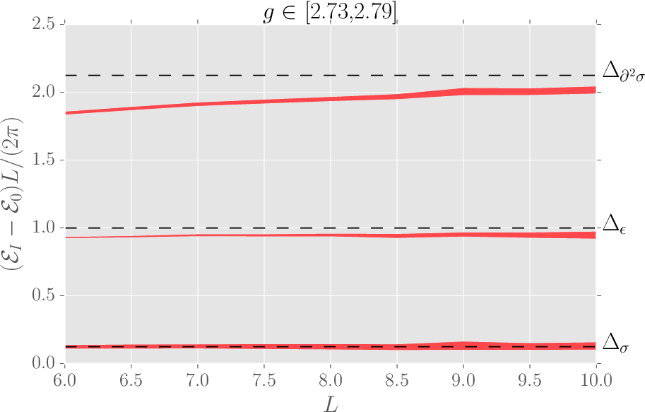
Finally, we compare the NLO-HT results to the expectations for the finite volume spectra at the critical point. CFT predicts that the energy levels at should vary with as
| (36) |
where are operator dimensions in the critical Ising model. This relation should hold at , where corrections due to irrelevant couplings die out. In Fig. 4 we test it for the first three energy levels above the vacuum, which should correspond to the operators with dimensions , , . The error comes from extrapolating to and (the largest contribution) from varying in the range (35). We see reasonable agreement for and , while it looks like the agreement for will be reached at higher values of . This figure can be compared to Fig. 6 of [12] and Figs. 22, 23 of [26], which show similar behavior.
Conclusions. In this work we proposed a variant of renormalized Hamiltonian Truncation called NLO-HT. Its main idea is to integrate out exactly a certain class of high-energy states, which allows for variational interpretation, and furthermore implements the renormalization corrections up to cubic order in the interaction strength.
We tested NLO-HT by computing the low-lying spectra of the strongly coupled two-dimensional theory. Numerical spectra in finite volume were found to converge rapidly with the Hilbert space cutoff , faster than for other existing versions of Hamiltonian Truncation, and allowing controlled extrapolation to the continuum limit . The finite volume corrections were then removed using the theoretical knowledge of these effects in QFT. In this way we extracted highly accurate predictions for the vacuum energy density and the physical mass in the infinite volume limit, for a range of non-perturbative coupling constants.
In the future NLO-HT will be used to perform accurate studies in other strongly coupled RG flows in . In particular, it can be applied to flows starting from an interacting CFTs. We also believe that our ideas will be useful to extend Hamiltonian Truncation to weakly relevant interactions, with scaling dimension in the range excluded in this paper, and in particular to flows in higher dimensions , most of which fall into this category.
Acknowledgements.
We thank Richard Brower, Ami Katz, Robert Konik, Iman Mahyaeh, Marco Serone, Gabor Takács, Giovanni Villadoro and Matthew Walters for the useful discussions. SR is supported by the National Centre of Competence in Research SwissMAP funded by the Swiss National Science Foundation, and by the Simons Foundation grant 488655 (Simons collaboration on the Non-perturbative bootstrap). The work of LV was supported by the Simons Foundation grant on the Nonperturbative Bootstrap and by the Swiss National Science Foundation under grant 200020-150060. The computations were performed on the BU SCC and SISSA Ulysses clusters.References
- [1] S. R. White, “Density-matrix algorithms for quantum renormalization groups,” Phys. Rev. B48, 10345 (1993).
- [2] D. Perez-Garcia, F. Verstraete, M. M. Wolf, and J. I. Cirac, “Matrix Product State Representations,” Quantum Inf. Comput. 7, 401 (2007), quant-ph/0608197 .
- [3] Y.-Y. Shi, L.-M. Duan, and G. Vidal, “Classical simulation of quantum many-body systems with a tree tensor network,” Phys. Rev. A74, 022320 (2006), quant-ph/0511070 .
- [4] G. Vidal, “Class of Quantum Many-Body States That Can Be Efficiently Simulated,” Phys. Rev. Lett. 101, 110501 (2008), quant-ph/0610099 .
- [5] F. Verstraete, V. Murg, and J. I. Cirac, “Matrix product states, projected entangled pair states, and variational renormalization group methods for quantum spin systems,” Advances in Physics 57, 143–224 (2008), arXiv:0907.2796 [quant-ph] .
- [6] V. P. Yurov and Al. B. Zamolodchikov, “Truncated Conformal Space Approach to Scaling Lee-Yang Model,” Int.J.Mod.Phys. A5, 3221–3246 (1990).
- [7] V. P. Yurov and Al. B. Zamolodchikov, “Truncated fermionic space approach to the critical 2-D Ising model with magnetic field,” Int.J.Mod.Phys. A6, 4557 (1991).
- [8] A. J. A. James, R. M. Konik, P. Lecheminant, N. J. Robinson, and A. M. Tsvelik, “Non-perturbative methodologies for low-dimensional strongly-correlated systems: From non-abelian bosonization to truncated spectrum methods,” arXiv:1703.08421 [cond-mat.str-el] .
- [9] In relativistic QFTs one can also quantize on surfaces of constant light-cone coordinate. This light front quantization [39] is also used in numerical solutions of strongly coupled QFTs via a version of HT; some recent work is [40, 41, 42, 43, 44, 45]. The structure of the unperturbed Hilbert space is different from the equal time case, which leads to important differences in the numerical procedure. All technical claims in this work will refer exclusively to the equal time quantization.
- [10] T. R. Klassen and E. Melzer, “Spectral flow between conformal field theories in (1+1) dimensions,” Nucl.Phys. B370, 511–550 (1992).
- [11] M. Hogervorst, S. Rychkov, and B. C. van Rees, “Truncated conformal space approach in dimensions: A cheap alternative to lattice field theory?” Phys. Rev. D91, 025005 (2015), arXiv:1409.1581 [hep-th] .
- [12] S. Rychkov and L. G. Vitale, “Hamiltonian truncation study of the theory in two dimensions,” Phys. Rev. D91, 085011 (2015), arXiv:1412.3460 [hep-th] .
- [13] S. Rychkov and L. G. Vitale, “Hamiltonian truncation study of the theory in two dimensions. II. The -broken phase and the Chang duality,” Phys. Rev. D93, 065014 (2016), arXiv:1512.00493 [hep-th] .
- [14] J. Elias-Miró, M. Montull, and M. Riembau, “The renormalized Hamiltonian truncation method in the large expansion,” JHEP 04, 144 (2016), arXiv:1512.05746 .
- [15] P. Giokas and G. Watts, “The renormalisation group for the truncated conformal space approach on the cylinder,” (2011), arXiv:1106.2448 [hep-th] .
- [16] G. Feverati, K. Graham, P. A. Pearce, G. Zs. Toth, and G. Watts, “A Renormalisation group for TCSA,” J. Stat. Mech. , P03011 (2008), arXiv:hep-th/0612203 [hep-th] .
- [17] G. Watts, “On the renormalisation group for the boundary Truncated Conformal Space Approach,” Nucl.Phys. B859, 177–206 (2012), arXiv:1104.0225 [hep-th] .
- [18] M. Lencses and G. Takacs, “Excited state TBA and renormalized TCSA in the scaling Potts model,” JHEP 09, 052 (2014), arXiv:1405.3157 [hep-th] .
- [19] Joan Elias-Miro, Slava Rychkov, and Lorenzo G. Vitale, “NLO Renormalization in the Hamiltonian Truncation,” Phys. Rev. D96, 065024 (2017), arXiv:1706.09929 [hep-th] .
- [20] This has to be distinguished from the Numerical Renormalization Group (NRG) improvement of the HT [46] à la Wilson’s NRG [47]. This method raises the cutoff by adding new chunks of the Hilbert space and tossing away the states which have low overlaps with the interacting eigenstates. Other ideas to extend the reach of HT include sweeping and reordering (see [8]). We have not used any of these interesting tricks in our work.
- [21] That can be intuitively understood as follows. For each , there will be states below the cutoff for which the matrix elements of grow as in absolute value, where is the occupation number of the state and is a constant. For big enough, the expansion is therefore not convergent, as the truncated matrix element will outgrow the leading order contribution of growing as . For a detailed discussion of this point see [19], appendix B.
- [22] In this work, we introduce a tail state for each . This limits the number of states we include in the basis, as the full matrix () needs to be inverted over the space of tail states. On the contrary, the low-energy diagonalization of is performed efficiently via the Lanczos method. This suggests that more efficient numerics could be achieved by reducing the number of tails states ; see [19] for a discussion.
- [23] In practice we fix to the value given by the local approximation mentioned below Eq. (12). Further iterative improvements are possible, but their effect is negligible.
- [24] By applying the power counting arguments mentioned in footonote 21, one can estimate , as opposed to , therefore taming the growth of the matrix elements.
- [25] A. Coser, M. Beria, G. P. Brandino, R. M. Konik, and G. Mussardo, “Truncated Conformal Space Approach for 2D Landau-Ginzburg Theories,” J. Stat. Mech. 1412, P12010 (2014), arXiv:1409.1494 [hep-th] .
- [26] Z. Bajnok and M. Lájer, “Truncated Hilbert space approach to the 2d theory,” JHEP 10, 050 (2016), arXiv:1512.06901 [hep-th] .
- [27] To estimate extrapolation errors, we fitted subsamples of the full data set, obtained by removing points at low in different combinations.
- [28] M. Lüscher, “Volume Dependence of the Energy Spectrum in Massive Quantum Field Theories. 1. Stable Particle States,” Commun.Math.Phys. 104, 177 (1986).
- [29] T. R. Klassen and E. Melzer, “On the relation between scattering amplitudes and finite size mass corrections in QFT,” Nucl. Phys. B362, 329–388 (1991a).
- [30] As a further check of the method, the S-matrix (extracted via the volume dependence of the spectrum) could in the future be compared to the perturbative prediction for . See [25], appendix B.
- [31] T. R. Klassen and E. Melzer, “The Thermodynamics of purely elastic scattering theories and conformal perturbation theory,” Nucl. Phys. B350, 635–689 (1991b).
- [32] S.-J. Chang, “The Existence of a Second Order Phase Transition in the Two-Dimensional Field Theory,” Phys.Rev. D13, 2778 (1976).
- [33] D. Schaich and W. Loinaz, “An improved lattice measurement of the critical coupling in theory,” Phys.Rev. D79, 056008 (2009), arXiv:0902.0045 [hep-lat] .
- [34] A. Milsted, J. Haegeman, and T. J. Osborne, “Matrix product states and variational methods applied to critical quantum field theory,” Phys.Rev. D88, 085030 (2013), arXiv:1302.5582 [hep-lat] .
- [35] P. Bosetti, B. De Palma, and M. Guagnelli, “Monte Carlo determination of the critical coupling in theory,” Phys. Rev. D92, 034509 (2015), arXiv:1506.08587 .
- [36] A. Pelissetto and E. Vicari, “Critical mass renormalization in renormalized theories in two and three dimensions,” Phys. Lett. B751, 532–534 (2015), arXiv:1508.00989 [hep-th] .
- [37] To compare with the critical coupling extractions using the light front quantization [42, 43, 45] one has to perform nonperturbative mass renormalization [43].
- [38] The central value corresponds to the smallest . The uncertainty interval was conservatively determined from the condition . Our determination is the best HT measurement of . It is compatible with and has accuracy comparable to other available determinations [19].
- [39] S. J. Brodsky, H.-C. Pauli, and S. S. Pinsky, “Quantum chromodynamics and other field theories on the light cone,” Phys.Rept. 301, 299–486 (1998), arXiv:hep-ph/9705477 [hep-ph] .
- [40] E. Katz, G. M. Tavares, and Y. Xu, “Solving 2D QCD with an adjoint fermion analytically,” JHEP 1405, 143 (2014a), arXiv:1308.4980 [hep-th] .
- [41] E. Katz, G. M. Tavares, and Y. Xu, “A solution of 2D QCD at Finite using a conformal basis,” (2014b), arXiv:1405.6727 [hep-th] .
- [42] S. S. Chabysheva, “Light-front theory using a many-boson symmetric-polynomial basis,” Proceedings, Light Cone 2015: Frascati, Italy, Sep 21-25, 2015, Few Body Syst. 57, 675–680 (2016), arXiv:1512.08770 [hep-ph] .
- [43] M. Burkardt, S. S. Chabysheva, and J. R. Hiller, “Two-dimensional light-front theory in a symmetric polynomial basis,” (2016), arXiv:1607.00026 [hep-th] .
- [44] E. Katz, Z. U. Khandker, and M. T. Walters, “A Conformal Truncation Framework for Infinite-Volume Dynamics,” JHEP 07, 140 (2016), arXiv:1604.01766 [hep-th] .
- [45] N. Anand, V. X. Genest, E. Katz, Z. U. Khandker, and M. T. Walters, “RG Flow from Theory to the 2D Ising Model,” (2017), arXiv:1704.04500 [hep-th] .
- [46] R. M. Konik and Y. Adamov, “Numerical renormalization group for continuum one-dimensional systems,” Phys. Rev. Lett. 98, 147205 (2007), arXiv:cond-mat/0701605 [cond-mat.str-el] .
- [47] K. G. Wilson, “The renormalization group: Critical phenomena and the kondo problem,” Rev. Mod. Phys. 47, 773–840 (1975).