Asymptotic and numerical analysis of a porous medium model
for transpiration-driven sap flow in treesThanks: Submitted to the editors DATE.
Abstract
We develop a 3D porous medium model for sap flow within a tree stem, which consists of a nonlinear parabolic partial differential equation with a suitable transpiration source term. Using an asymptotic analysis, we derive approximate series solutions for the liquid saturation and sap velocity for a general class of coefficient functions. Several important non-dimensional parameters are identified that can be used to characterize various flow regimes. We investigate the relative importance of stem aspect ratio versus anisotropy in the sapwood hydraulic conductivity, and how these two effects impact the radial and vertical components of sap velocity. The analytical results are validated by means of a second-order finite volume discretization of the governing equations, and comparisons are drawn to experimental results on Norway spruce trees.
keywords
tree sap transport, porous media flow, asymptotic series, finite volume method.Funding.
This work was funded in part by a Discovery Grant from the Natural Sciences and Engineering Research Council of Canada and a grant from the North American Maple Syrup Council Research Fund.AMS
35C20, 35K61, 76M12, 76S05, 92C05, 92C80.1 Introduction
The phenomenon of sap transport in trees has challenged plant physiologists for over a century [11]. The remarkable ability of trees to draw water upward from roots to leaves through heights of 100 metres or more is still not completely understood and still generates a great deal of interest in the biophysics and plant physiology communities [1, 6, 17]. The driving process behind sap flow is transpiration, which can be briefly explained as follows [34]. Water is lost from the leaves as a consequence of the shared path between inward diffusion of carbon dioxide (the essential precursor for photosynthesis) from the ambient air to the leaves, and the combined outward evaporation/diffusion of water due to the vapor pressure deficit. As water evaporates from the leaves, air-water surface tension is generated within the hydrophilic leaf cell interstices and is subsequently transmitted through the sap to conductive wood cells (known as sapwood or xylem) making up the stem and branches. The resultant negative sap pressure (measured relative to atmospheric) generates the driving force necessary to draw water from the roots to the leaves [27]. This transpiration-driven flow is a maximum during the day when there is a high evaporative demand, and drops to a minimum overnight when photosynthesis halts and the internal water storage within the tree is replenished [39].
The physical structure of wood plays an essential role in sap transport. Within coniferous (or softwood) tree species that are the focus of this study the primary conductive elements in sapwood are the tracheids, which are elongated and vertically-oriented dead wood cells having rigid lignified cellulose walls enclosing an empty lumen. Adjacent tracheids are hydraulically connected through paired pits, which are pores that permit flow of liquid sap but are small enough to prevent passage of any air bubbles that might be formed within the tracheids. When the sapwood is viewed as a porous medium, the combination of pit distribution and tracheid orientation engenders a high degree of anisotropy in hydraulic conductivity, which can be several orders of magnitude larger in the vertical direction than the radial [8]. Deciduous (or hardwood) tree species differ from conifers in that sapwood contains an extra class of wood cells called vessels having a much larger diameter and with greater permeability to flow, although the wood structure and transport properties remain otherwise similar.
Because typical pressures within a tree stem exceed the saturated vapor pressure, gases such as air and carbon dioxide are known to exist in a dissolved state within the sap. Under conditions of extreme dryness or freezing, pressure can fall enough to cause dissolved gases to cavitate and form air bubbles inside tracheids or vessels [39]. This process is known as embolism and can lead to blockage of affected conduits that prevents them from conducting sap. Trees have an amazing microstructure that is capable of bypassing and even eliminating such embolisms [10], but the precise mechanisms for embolism formation and recovery are still not completely understood [5]. To avoid having to model the added complexities of embolism formation, we assume in this study that the trees operate under “normal conditions” in which the sapwood remains close to full saturation so that no new embolus forms, and neither does embolism recovery play a significant role.
Numerous mathematical have been developed for studying the flow of sap within conductive sapwood. One of the most popular approaches is an electric circuit analogy, in which the porous flow elements are characterized by a flow resistance (which is inversely proportional to conductivity), combined with capacitive elements that capture storage of sap (and subsequent time lags) within the roots, leaves and various cells making up the stems and branches [14]. The earliest circuit models included only resistive elements and hence failed to capture the dynamic nature of the flow [37], whereas more recent models include water storage effects and hence capture observed lags between transpiration flux and sap flow [26]. Some authors have developed even more detailed models that capture the branching structure of the tree [36], or incorporate the added dynamic effects of radial stem growth [32] by connecting resistor-capacitor elements in a more complex branching structure. A major drawback of these circuit models is that the parameters have no direct correspondence in the context of an actual porous medium flow, and the resistance and capacitance are treated instead as fitting constants that are matched to experiments rather than being directly measured. Furthermore, the circuit analogue is constructed out of a network of resistors and capacitors connected in series, for which the resulting flow depends sensitively on the actual discretization used. Finally, the circuit parameters are usually treated as constants although the transport properties of actual sapwood change in time owing to the local saturation state. Having said that, circuit models are still applied widely in the tree physiology literature because of their simplicity and straightforward algebraic structure.
Another type of model that overcomes many of these deficiencies is the class of porous medium models. The study of unsaturated porous flow in porous media is very well developed [20], especially in the context of groundwater transport in soils [9]. Sap flow is especially suitable for treatment using continuum porous medium models because of the simple repeating microstructure of wood. In this class of models, sap flow is driven by pressure gradients according to Darcy’s law, and the governing equations consist of nonlinear partial differential equations (PDEs) that capture spatial and temporal variations in variables such as water content (saturation) and pressure. Chuang et al. [7] developed a simple 1D porous medium model for transpiration driven flow in a conifer stem, and used numerical simulations to fit their results to experimentally measured sap fluxes. Bohrer et al. [4] extended these results to include the effect of complex branching structure within the crown [7]. Aumann and Ford [2, 3] applied a different approach focused on the wood microstructure in Douglas fir by developing a detailed model for transport within a tracheid network including water-air interface dynamics and many microstructural parameters. Such a model is useful for uncovering detailed aspects of flow within individual wood cells, but it is not very practical for use at the scale of an entire tree. A number of other related PDE models have been also developed [13, 21, 25, 30], but many are one-dimensional and so ignore effects such as radial variations within the stem, not to mention that to date little mathematical analysis has been done to determine the character of the solutions.
The main goal of this paper is to extend the 1D porous medium model from [7] to a more realistic 3D cylindrical (rotationally symmetric) model of a tree trunk, with an imposed transpiration flux distributed along the outer surface. Along with realistic coefficient functions fit to data on Norway spruce, this model will permit study of the radial flow patters that develop with the stem. We will then develop an approximate analytical solution with the aid of asymptotic analysis, identifying the different parameter regimes where anisotropy begins to dominate which provides an alternate explanation for the observed radial variation in the vertical velocity [15, 28] that isn’t due to loss of hydraulic conductivity. We study the relative importance of gravity and transpiration as well as investigating the nature and relative importance of the radial/vertical sap fluxes, which is significant in light of the recent experimental advances that permit measurements of the relatively small radial sap velocity components [12, 35]. We further demonstrate how temporal and spatially localized disturbances in saturation propagate along the tree. Throughout, we use a finite volume discretization of the governing nonlinear PDE in order to solve the problem numerically and validate the asymptotic results.
2 Model for 3D Axisymmetric Flow in a Tapered Cylindrical Annulus
Our work is based on the one-dimensional sap flow model of Chuang et al. [7], who considered only vertical variations within a tapered cylindrical tree stem. We extend their model to a 3D axisymmetric stem geometry by incorporating the effect of radial variations as well as a core heartwood region that is impermeable to flow. Except for slight changes in notation and the need for several additional boundary conditions, the model is much the same as the 1D analogue. A description of all parameters and solution-dependent coefficient functions is provided in section 2.2, which are obtained from the literature or fit to experimental measurements from Norway spruce (Picea abies) provided in [7].
2.1 Governing Equations and Boundary Conditions
The Norway spruce is a conifer species whose stem is well-approximated by a right circular cylinder that tapers from base to crown. For a tree of height (in units of ) the outer stem radius may be written as , where the axial coordinate satisfies and is a decreasing function of (which will be specified later in section 2.2). We extend the 1D model from [7] by taking a more realistic geometry pictured in fig. 1a where the stem consists of an outer layer of conducting sapwood that surrounds a core region of non-conducting heartwood. The heartwood is assumed to take up some fraction of the stem cross-section corresponding to . We are therefore concerned with capturing sap transport within the outer conductive portion which has the shape of a tapered cylindrical annulus defined by
| (2.1) |
In the absence of any directional forcing around the stem, we can suppose rotational symmetry and neglect any dependence on the polar angle.
| (a) | (b) | |||
|---|---|---|---|---|
 |
 |
The sapwood is treated as a variably-saturated medium whose porous structure contains a mixture of two phases: liquid (sap) and gas (mostly air). The saturation or local pore volume fraction containing liquid is denoted by , and depends on location and time . Enforcing conservation of liquid yields the continuity equation
| (2.2) |
where the sap velocity obeys Darcy’s law
Here is the hydrostatic pressure head, which is a saturation-dependent function that is specified later in section 2.2. The hydraulic conductivity tensor depends in general on both the location within the tree stem (due to spatial variations in pore structure) and the local saturation state. The porous structure of wood is highly anisotropic since it is composed of dead, hollow, elongated cells that are directed vertically within the xylem; in conifers, these cells are tracheids, whereas in deciduous trees the primary route for sap transport is through much larger cells called vessels. Microscopic “pits” or pores connect adjacent wood cells in the radial direction, as well as a much smaller number of radially-directed “ray cells”; however, these structures are much less permeable to flow than the vertically-oriented tracheids, so it is reasonable to assume that the anisotropic hydraulic conductivity has the form of a diagonal tensor
| (2.3) |
Note that depends on position but not on saturation, which we justify based on the earlier assumptions that sapwood remains nearly saturated and no significant build-up of gas occurs owing to absence of embolism formation. This should be contrasted with Chuang et al. [7] who took the conductivity to be a function of saturation; however, since we are primarily concerned with trees near the fully saturated state where the hydraulic conductivity is relatively insensitive to changes in , taking to be independent of is a reasonable approximation (to be discussed more detail in the next section).
In most trees, the dominant vertical orientation of conductive cells induces anisotropy in that ranges from moderate to extreme. Therefore, the analytical derivations in this paper focus on two limiting cases: an isotropic conductivity with , for which a general series solution is relatively straightforward to derive; and high anisotropy with , which can be treated analytically under certain restrictions. In either case, numerical simulations are used to study the solution over the entire range of anisotropy.
Using the above definitions, the velocity can be expressed in cylindrical coordinates as
| (2.4) |
After substituting these two expressions into the continuity equation eq. 2.2, we obtain the following nonlinear parabolic PDE for saturation
| (2.5) |
Moving on to the boundary conditions, no sap flows through the top of the stem so that
| (2.6) |
whereas the base of the stem (at the roots) is assumed to be fully saturated with
| (2.7) |
On the inner sapwood boundary, a zero flux is imposed
| (2.8) |
where is the unit outward-pointing surface normal. This last condition reflects the fact that no sap exchange occurs with the non-conducting heartwood (and reduces to a simple radial symmetry condition in the case ).
The final boundary condition on the outer stem surface derives from the transpiration flux, which is the process whereby water is drawn upward from the roots, through the stem and branches to the leaves (or needles). Transpiration is driven by leaf evaporation and the subsequent vapor pressure deficit between the leaf interior and the surrounding atmosphere. A particular feature of species like Norway spruce is that branches are distributed densely along the entire stem so that the transpiration flux can be specified as a corresponding distribution in the axial direction (this should be contrasted with many deciduous species in which branches are concentrated within the crown at the top of a long, bare trunk). Therefore, we impose a sap outflow due to branches distributed continuously along the stem by means of another flux boundary condition
| (2.9) |
The transpiration flux depends on time owing to diurnal variations in transpiration, as well depending on the branch distribution along the stem, and we provide a specific functional form for in the next section. A primary difference from the 1D model in [7] is that the transpiration flux was incorporated as a source term in the saturation equation eq. 2.5 rather than as a boundary condition. A graphical summary of the geometry and boundary conditions is provided in fig. 1b.
2.2 Parameters and Coefficient Functions
We now provide parameter estimates and functional forms for the model coefficients, which are chosen to match as closely as possible the data for Norway spruce provided in [7]. All symbols are listed in table 1 along with units and values. We emphasize that neither the model nor the asymptotic analysis in the following sections is restricted to a particular species of tree, and that the specific functional forms introduced here are not critical for the analysis. Rather, we exploit these parameters as a convenient illustration of our 3D model, which has the added benefit of allowing us to draw a concrete comparison with the results in [7].
| Symbol | Description | Units | Value or Formula |
|---|---|---|---|
| Independent and dependent variables: | |||
| radial coordinate | |||
| vertical coordinate | |||
| time | |||
| sap volume fraction or saturation | – | ||
| saturation deficit | – | ||
| radial sap velocity | |||
| vertical sap velocity | |||
| Solution-dependent functions: | |||
| transpiration rate per unit leaf area | eq. 2.13b | ||
| combined leaf area and shading effects | – | eq. 2.13c | |
| hydraulic conductivity tensor | eq. 2.3 | ||
| hydraulic conductivity components | eq. 2.11 | ||
| leaf area per unit height | eq. 2.13d | ||
| outer stem radius | eq. 2.10 | ||
| sunlight shading effect | – | eq. 2.13e | |
| capillary pressure head | eq. 2.12 | ||
| Physical (dimensional) parameters: | |||
| transpiration flux amplitude | () | ||
| stem height | 6.7 | ||
| maximum hydraulic conductivity | |||
| leaf specific area | 15.3 | ||
| maximum tree radius (at base) | 0.0645 | ||
| number of seconds per day | |||
| scaling constant in | |||
| Dimensionless parameters: | |||
| maximum of | 2.6 | ||
| capillary pressure exponent | 400 | ||
| maximum saturation | 0.574 | ||
| exponential stem taper rate | 1.42 | ||
| heartwood fraction (inner : outer radius ratio) | 0 (0–0.75) | ||
| relative change from max. saturation | 0.01 | ||
| stem aspect ratio | 0.00963 | ||
| time parameter | |||
| conductivity ratio | – | ||
| gravity parameter | 0.00915 | ||
| transpiration parameter | 0.00920 (0.363) | ||
We first specify the form of the outer tree stem radius that tapers with height according to
| (2.10) |
where controls the rate of taper from roots to crown. This choice of exponential function was motivated in [7] for reasons of mathematical convenience. However, there is an extensive literature on more complicated diameter-versus-height relationships [22, 24], from which we observe that many coniferous and deciduous tree species have a small enough taper rate that such an exponential function provides a reasonable approximation of stem shape. However, we still develop the majority of our analytical results for the general function and impose eq. 2.10 when we need to exploit additional simplifications in section 4.6, and in numerical simulations when a specific form of is required.
Another important geometric parameter is the heartwood ratio that determines the thickness of the annular sapwood region. For young trees that have not yet developed a well-defined heartwood region, taking is a reasonable choice. For spruce trees of the age and height considered in [7] the typical heartwood fraction is [31], while for other species can be as high as 0.75 [38]. For most of this paper including the asymptotic developments we assume that , although we explain later how our results can be extended to the case when the heartwood fraction is much larger.
Based on our earlier assumption that the hydraulic conductivity is a diagonal tensor with entries that depend only on position, we take the axial and radial conductivities to have the form
| (2.11) |
where is a constant equal to the maximum value of axial hydraulic conductivity, and is a dimensionless function that is strictly positive. The dimensionless factor is the ratio of radial to axial conductivity that captures the degree of anisotropy in the sapwood. Typical values of lie between to [8, 29], although we will also consider the case when (where we use to denote asymptotic equivalence in which the two quantities have the same order of magnitude).
Many models of variably-saturated porous media specify the hydraulic conductivity as a function of saturation; indeed, Chuang et al. [7] imposed a Weibull-type function of the form . However, their simulations remained within 20% of the fully saturated state , for which has a nearly linear dependence on with a very small (negative) slope. The reason for this behaviour is that the primary cause of hydraulic conductivity loss in trees is embolism formation, which only occurs when saturation drops sufficiently below . Since we expect that variations in saturation remain relatively small, it is reasonable to approximate variations in conductivity using a simpler spatially dependent function for which we derive most of our asymptotic results (and which avoids a nonlinear ). After investigating the asymptotic solution for spatially-dependent conductivity, we then consider in section 4.6 the special case of constant conductivity and a periodic transpiration rate, which allows us to derive a simpler closed–form solution for the leading order term.
The hydraulic pressure head is taken to depend on saturation according to
| (2.12) |
where and are fitting parameters. This is similar to the van Genuchten model commonly used for capillary pressure in soil and rock [33], and also applied to drying of lumber [18]. Note that the head is a negative quantity because , reflecting the understanding in the sap hydraulics literature that sap within a tree stem is under tension. Our asymptotic derivation is not specific to this or any other particular form of the capillary pressure function, but does rely on two essential features: namely, that is a smooth and monotone increasing function in a neighbourhood of .
The final ingredient in the model specification is the transpiration source term, which we assume takes the separable form
| (2.13a) | |||
| where captures time variations throughout the daily transpiration cycle while embodies changes with height. In general, our only requirement on the source term is that the time-dependent factor is periodic and can be expressed as a Fourier series; however, for illustration purposes we choose particular forms for both functions that approximate the experimental data provided in [7]. For the time-dependent factor we take a periodic function | |||
| (2.13b) | |||
| consisting of a three-term Fourier expansion, where time is measured from midnight on the first day, is the diurnal period, and is the amplitude of the transpiration flux. The complex fitting parameters and are obtained by digitizing 36 data points from [7, Fig. 7 (bottom, CC)] and then using a discrete Fourier transform to extract the first three Fourier coefficients, which are sufficient to obtain a smooth approximation of the original data. | |||
The height-dependent transpiration factor is decomposed as
| (2.13c) |
where is a geometric scaling factor (equal to stem perimeter) and is leaf area density (units of ) that captures the impact of sun exposure on transpiration and is given in [7, Fig. 4] as
| (2.13d) |
The remaining factor is a dimensionless quantity called transpiration flux density that captures shading effects due to branches/leaves located above a given height. Although was not provided in [7], it can be approximated using experimental data in [7, Fig. 5] as
| (2.13e) |
3 Numerical Method
We next describe a numerical method for solving the governing equations based on a cell-centered finite volume approximation. This will be used to validate our asymptotic results in the case of an isotropic conductivity, and to produce comparisons for the anisotropic case. To simplify the discrete equations, it is helpful to first transform the radial coordinate for the tapered annular cylindrical domain.
3.1 Coordinate Transformation
The radius of the tapered cylinder obeys , which suggests defining a transformed radial coordinate that is bounded between for all . The spatial derivatives within the governing equations can then be transformed via
where is a constant owing to the special exponential form eq. 2.10 assumed for . Applying these transformations to the velocity components eq. 2.4 yields
| (3.1) |
where . Here the velocities are written in terms of a general saturation dependent hydraulic conductivity function , which is useful for later comparison to the results in [7] (see section 3.3); however, the same formulas extend easily to a spatially-dependent conductivity . Making use of these velocity components, the continuity equation eq. 2.5 becomes
| (3.2) |
The primary advantage to transforming the radial coordinate in this manner is that the equations above are now imposed on a rectangular computational domain in space, for which standard finite difference approximations can be applied.
3.2 Cell-centered Finite Volume Discretization
We now discretize the transformed governing equations using a cell-centered finite volume scheme, so that we preserve as accurately as possible the conservation of mass embodied in the continuity equation. The computational domain is divided into an rectangular grid of cells having centers
| (3.3) |
with and for and . As shown in fig. 2, the saturation is approximated at cell centers, whereas the velocity components are located at the center of each cell edge, denoted for example by and . The spatial derivatives in eq. 3.1 are then replaced using compact centered difference formulas to obtain edge-centered velocities
| (3.4) | ||||
| (3.5) | ||||
| (3.6) |
Note that to maintain both stencil compactness and second-order accuracy we have had to introduce approximate values of saturation at cell edges and corners along with corresponding approximations for , all of which are computed using appropriate arithmetic averages of cell-centered saturation values. The velocity components are then substituted into the discrete continuity equation to get
| (3.7) |
To discretize the boundary conditions, we set the normal velocity at the center of each boundary cell edge to the velocity specified in the corresponding boundary conditions eq. 2.6, eq. 2.8 and eq. 2.9. As for the remaining lower boundary, we introduce a band of fictitious cells with centers located one-half grid spacing below the boundary and define values of saturation at these fictitious points. Using the boundary cell values and the lower boundary edge value in eq. 2.7, a linear extrapolation is used to calculate the saturation in the fictitious cells. Complete details of the spatial discretization are provided in [16]. To integrate the equations in time, we use a method-of-lines approach in which the spatially-discrete equations are treated as a system of time-dependent ODEs, which is then integrated in time using Matlab’s stiff ODE solver ode15s with tolerance values .

In order to verify that our Matlab implementation yields the desired order of spatial accuracy, we performed a numerical convergence study by choosing a sequence of spatial grids with and computing the solution on a fixed time interval that roughly reaches a steady state. The error for each simulation is estimated by treating the fine-grid solution as the “exact solution” and then calculating the 1-norm difference. The resulting errors exhibit a convergence rate of approximately 1.99 which is strongly indicative of second-order accuracy.
3.3 Comparison With Experimental Data on Norway Spruce
We now compare results from the 3D numerical scheme with the experimental data on vertical sap flux provided by Chuang et al. [7]. For this simulation, we use parameters listed in table 1, except that in order to be consistent with the 1D model we assume the entire stem is made of conductive sapwood () that is isotropic (). Figure 3a depicts the measured sap flux (in the vertical direction) alongside our finite volume simulations at two different times (noon and 4:00 pm). The model results clearly capture the overall solution behaviour, exhibiting the same “double-peak” behaviour in sap flux that can be attributed to the bimodal behaviour of the transpiration function from eqs. 2.13c to 2.13e (shown in fig. 3b). In addition to this qualitative agreement, we note that the magnitude of the sap flux is also reasonably well-approximated by computations. Simulations of the 1D model equations of Chuang et al. were also performed using an analogous finite volume scheme and the results were indistinguishable to the eye from the results in fig. 3.
| (a) | (b) | (c) |
|---|---|---|
 |
 |
 |
The primary reasons for developing this 3D sap flow model are to capture radial velocity (as well as radial variations in the solution) and to investigate the impact of including a non-conducting heartwood region with . With this in mind, we performed a series of three simulations with different heartwood thickness (, 0.5 and 0.75) and plotted the resulting radial velocities in fig. 4. Two positive peaks appear in which clearly derive from the local maxima in the transpiration flux, and these are offset by a comparatively large negative radial velocity at the tree base due to root influx. This is a geometric effect that mimics the inward radial tilt of sapwood vessels, which due to stem taper is largest at the base. The effect of this radially-inward flow is accentuated as the thickness of the annulus decreases (i.e., as increases) in order to maintain a total mass balance that matches the specified outward transpiration flux.
| (a) | (b) | (c) |
|---|---|---|
 |
 |
 |
4 Asymptotic Analysis
The asymptotic derivation in this section bears some resemblance to Kevorkian and Cole’s analysis of heat conduction in a long circular rod [19, chapter 4]. Our results hold for the general case of sap flow in an annular stem cross-section eq. 2.1 as well as a saturation-dependent conductivity, and we make no assumption on the functional form of either or the transpiration flux defined via and . However, for the time-varying solution we will exploit simplifications that arise from assuming an exponential taper eq. 2.10 and constant hydraulic conductivity. We begin by considering the special case when the radial and axial conductivities and are the same order of magnitude so that , and defer study of the anisotropic case to section 4.5.
4.1 Non-Dimensionalization in the Nearly-Saturated Regime
We next recast the 3D model in dimensionless form in order to reduce the number of free parameters and identify important dimensionless groupings (an analogous version of the 1D model can be derived as well, be we don’t present it here). Introduce the following non-dimensional variables
| (4.1a) | |||
| as well as rescaled versions of the stem radius and transpiration functions | |||
| (4.1b) | |||
| where chosen equal to the maximum value of so that . Finally, we assume that the tree remains close to a fully saturated state so that the saturation variable may be written | |||
| (4.1c) | |||
where measures the relative deviation from full saturation and typically satisfies . In practice, increases with transpiration rate , although its precise value is not so important since ultimately cancels out from the final result in our asymptotic derivation. A rough estimate for can be found by recognizing that the threshold pressure for embolism in spruce has been measured as [23], corresponding to a saturation of . Because we are interested in “normal” flow conditions that are well-removed from any embolized state, we should thus constrain . In particular, using a “base value” of , simulations yield a so that saturation is guaranteed to remain close enough to (further discussion of is provided at the end of this section).
This rescaling has been performed such that and all “starred” variables can be considered quantities. Before rescaling the governing equations, we note that the hydrostatic pressure derivative appears in the saturation equation eq. 2.5 and the velocity boundary conditions through the Darcy velocities eq. 2.4. Because depends nonlinearly on saturation in eq. 2.12, we will ultimately need to expand as a power series as well. Therefore we perform this expansion step for now, which will also permit us to determine an appropriate set of dimensionless parameters that characterize the problem. To this end, we change variables using eq. 4.1 and expand , as power series in to obtain
| (4.2a) | ||||
| (4.2b) | ||||
where and (recalling that is large). Next, substitute the rescaled variables eq. 4.1 into the saturation equation eq. 2.5, which after rearranging yields
noting that only the first two terms in the series eq. 4.2 are required. Upon careful consideration of the various factors multiplying each term, we are led to introduce the following three dimensionless ratios
| (4.3) |
The parameter has an obvious physical interpretation as the stem aspect ratio and will play a central role as the primary expansion parameter in our asymptotic analysis. The rescaled saturation equation may be rewritten in terms of these parameters (after dividing by ) as
| (4.4) |
where all “stars” have been omitted on dimensionless quantities to streamline notation. For transpiration-driven flow we are interested only in the case where gravitational effects are significant at leading order, which means that the final term in eq. 4.4 must have . This implies that all terms are balanced except possibly the second, whose relative importance depends on the anisotropy parameter through the ratio – in practice, varies between and although we will begin considering the lower limit in the asymptotics.
We next consider the boundary conditions and assume for the present that in eq. 2.1, which corresponds to a stem consisting entirely of conducting sapwood (i.e., no heartwood). This does not restrict the generality of our results since we can still capture the effect of by introducing an appropriate spatial variation in . Taking introduces a major simplification in that the non-dimensional form of eq. 2.8 becomes
| (4.5) |
The corresponding top and bottom boundary conditions eqs. 2.6 and 2.7 become respectively
| (4.6) |
It is in this second boundary condition that the earlier assumption of ensures that the gravitational effects also contribute to the top boundary condition at leading order.
The derivation of the transpiration flux condition eq. 2.9 at the outer trunk surface is complicated by the presence of the curved boundary where the normal direction is not aligned with a coordinate axis. After changing variables and expanding terms involving , this boundary condition reduces to
| (4.7) |
where we have introduced the new dimensionless parameter
| (4.8) |
which means that . Thus, based on the “base value” for , the primary dimensionless parameters obey the equivalence . We note nonetheless that the asymptotic solution still yields an accurate approximation for much larger values of that violate this equivalence, which we will see later in fig. 9.
Because of the small aspect ratio, the radial and vertical components of the outward-pointing normal may be expanded as power series in small :
These expressions are exploited in the next section to simplify the boundary condition eq. 4.7.
4.2 Asymptotic Expansion: General Case
Based on the assumption that the saturation in eq. 4.1c stays close to its maximum value , we seek a regular power series expansion of in terms of the small parameter as
| (4.9) |
Our aim is to derive equations for the first two terms and so as to capture the effect of the nonlinearity in pressure head eq. 4.2a. We will also require two additional terms up to (involving and ), which are needed for matching purposes to obtain a closed set of equations for and . Furthermore, we will see shortly that the two leading order solutions are independent of so that is also required to determine the leading order term in the radial sap velocity. Taking the above expansion for saturation, the leading order equation from eq. 4.4 at is simply
Because conductivity must be nonzero, it follows that is independent of the radial coordinate and so . The same equation governs at , so we conclude likewise that . Considering the boundary condition eq. 4.7 at , if transpiration is to have any effect on saturation at the first two orders and (where the radial derivative term vanishes) then the remaining terms should balance. This is equivalent to requiring , which is satisfied for the parameters in table 1 with as discussed at the end of section 4.1.
The next order equation in eq. 4.4 involving terms at is
| (4.10) |
which can be integrated in and then evaluated at to obtain
Taking the same order terms arising in the transpiration boundary condition eq. 4.7 yields
| (4.11) |
where the last term is included at this order because . Eliminating from these last two equations leads to
which simplifies to
| (4.12) |
where we have defined
| (4.13) |
Equation eq. 4.12 can then be solved subject to the leading order boundary conditions from eq. 4.6:
| (4.14) |
Next we consider the terms in eq. 4.4 which lead to the equation
where we used the fact that . Integrating from to and evaluating at yields
and a second expression for comes from the boundary condition at the corresponding order in eq. 4.7
These last two equations can be combined to eliminate , and then further simplified by applying eq. 4.11 to obtain
Finally, using the fact that and are independent of , the integral terms can be evaluated and the governing PDE written in the more compact form
| (4.15) |
This PDE can be solved for provided that we impose appropriate boundary conditions, which are obtained from the terms in eq. 4.6 as
| (4.16) |
Note that the two terms in the top boundary condition are in balance only if , which is satisfied to a very good approximation.
4.3 Steady State Solution (Constant Transpiration Rate)
Explicit solutions can be derived for the two leading order asymptotic terms in the special case where the transpiration rate is constant () and the saturation has reached a steady state. In this case, the equation eq. 4.12 can be integrated twice using the boundary conditions eq. 4.14 to obtain
| (4.17) |
The first term in represents the effect of gravity due to changes in pressure with height. The second term captures the net effect of transpiration, where the expression in square brackets denotes total transpiration flux due to branches located above height , evaluated per unit stem conductivity. The next order saturation correction is obtained by integrating eqs. 4.15 to 4.16 in a similar manner, yielding
| (4.18) |
It is insightful at this point to draw an analogy between the formula for the leading order saturation and electric circuit representations commonly used to model tree sap hydraulics. To this end, we neglect the effects of gravity in eq. 4.17 and rewrite the remaining integral term as
| (4.19) | |||
can be interpreted as an average resistance to flow within the cross-sectional stem slice lying between and . This expression has the form of a harmonic average of conductivities , which is analogous to the formula relating electrical resistances and conductances arranged in a series circuit. The corresponding “current” is
which represents the total transpiration rate drawn through branches between and . The product is integrated in eq. 4.19 along the height of the tree in order to obtain the sap potential (or “voltage”), which when properly scaled yields the local saturation state.
4.4 Steady State Solution With Constant Conductivity
Our aim in this section is to estimate the ratio of radial to axial sap velocity and show that the reduction in radial-versus-axial flow is primarily due to the small stem aspect ratio () and not the conductivity ratio () as one might expect. We have already exploited the fact that variations in hydraulic conductivity with saturation are small by assuming that varies only with location. We now assume further that spatial variations in are likewise small so that it is reasonable to take the conductivity function .
Based on this assumption, eq. 4.10 may be integrated to obtain , which is the first term contributing to the radial velocity and also the lowest-order term containing any radial dependence. The resulting equation at steady state obeys
which may be substituted into eq. 2.4 along with earlier approximations and (4.17) to obtain a leading order expression for the (dimensional) radial velocity
| (4.20) |
Note that the conductivity ratio is absent from this expression for , which explains our earlier remark that the anisotropy only influences the radial velocity via higher order terms in the asymptotics.
Moving on to the axial velocity, we make use of the fact that when is constant equation eq. 4.13 reduces to , which leads to a simpler form of in eq. 4.17 that gives the leader order saturation derivative as
This expression can then be substituted into the axial component of eq. 2.4 and simplified to obtain the estimate
| (4.21) |
The relative magnitude of the two velocity components may then be approximated by
| (4.22) |
after dropping any terms. Consequently, the velocity ratio at steady state depends to leading order solely on stem aspect ratio, and furthermore the radial velocity is a factor of roughly 100 times smaller than the vertical component. The effect of material anisotropy on sap flow (through small ) has no impact at leading order, instead entering only via higher order terms in the asymptotics. This is the main reason that in earlier sections we restricted the asymptotic analysis to the case , since taking only pushes the effects of the anisotropy to higher order without impacting the leading order solution.
To illustrate these asymptotic results, we present in fig. 5a,b plots of the vertical velocity and saturation, determined using the two leading order terms in the steady state asymptotic solution. In both cases, the solution variables are averaged across the stem cross-section, and the corresponding finite-volume numerical solution is included in order to demonstrate the close correspondence. The vertical velocity exhibits the characteristic double peak that was observed for the variable-transpiration problem in fig. 3. To illustrate the relative magnitude of the velocity components, fig. 5c depicts the log of the ratio . Except for a thin boundary layer adjacent to the top boundary the radial component is at least a factor of 100 smaller than the vertical component, which is consistent with our asymptotic estimate of in eq. 4.22. The final plot in fig. 5d provides a clearer picture of the actual flow direction within the stem by depicting both streamlines and direction field arrows.
| (a) Average | (b) Average | (c) Log velocity ratio | (d) Velocity vector plot |
|---|---|---|---|
 |
 |
 |
 |
4.5 Anisotropic Conductivity With
Our earlier assumption that the hydraulic conductivity ratio is led to an asymptotic result in which the two leading order saturations and were independent of the degree of anisotropy in . However, sapwood is in reality a highly anisotropic material with [8, 29], which leads us to ask how taking values of might alter the asymptotic solution behaviour. In particular, the physical values of anisotropy and expansion parameter suggest considering two asymptotic limits: and . For reasons of simplicity, we will continue assuming that the conductivities are constant and the solution is at steady state.
First, consider the case of moderate anisotropy with , which corresponds to taking and (which we note is only an order of magnitude estimate and doesn’t presume any explicit dependence of on ). The saturation equation eq. 4.4 then becomes
and expanding in the form of a power series eq. 4.9 yields the leading order solution , which is identical to that obtained in the previous section. However, the next order equation for contains an additional term that introduces a radial dependence of the form
| (4.23) |
where the function is determined similarly as in the previous section (so we omit the details here).
In the second case of a more extreme anisotropy with , the saturation equation eq. 4.4 becomes
so that the radial and vertical dependence are now fully coupled at all orders. Assuming for simplicity that the stem has no taper (i.e., and ) we may transform the leading order solution using , which yields Laplace’s equation in cylindrical coordinates, along with boundary conditions
The advantage of transforming in this manner is that the boundary conditions become homogeneous, and hence separation of variables may be applied to obtain the series solution
where , is the zero’th order modified Bessel function of the first kind and
The effect of anisotropy on the solution is investigated in fig. 6 where we compare the simulated vertical velocity profiles for , using the three exponents and taking 6 terms in the Fourier–Bessel series for . These results are computed assuming a tree with no taper () and constant transpiration rate. For each , we plot as a function of radius at five heights corresponding to the points labelled A–E in fig. 3b. For the isotropic or moderately anisotropic cases () the velocity remains essentially constant with radius, whereas the extreme case of exhibits significant radial variations. This is consistent with our asymptotic results which show that radial dependence only enters the leading order solution when , and may help to explain the radial dependence in velocity that was observed experimentally in [15, 28].
This sequence of simulations was then repeated for a tapered stem with and the corresponding velocity plots are shown in fig. 7. We observe similar behaviour to the previous cases except that the results have a more pronounced radial variation. Even for the moderately anisotropic case (), there is a slight radial dependence visible in the bottom-most plot (location A). It is also interesting to note that introducing stem taper causes a significant drop in vertical velocity near the tree base owing to the increase in sapwood cross-section there; this should be comtrasted with the untapered case where the vertical velocity increases monotonically with height.
| (a) | (b) | (c) |
|---|---|---|
 |
 |
 |
| (a) | (b) | (c) |
|---|---|---|
 |
 |
 |
We performed one further validation of in the extreme case by comparing a numerical simulation with the 6-term series solution section 4.5. The relative difference in the saturation deficit between the asymptotic and numerical solutions is of order , which is the same order as the missing correction term in the asymptotic expansion of , as expected.
4.6 Time-Dependent Transpiration Source
Next, consider a more general time-dependent source where the transpiration rate is expanded as a Fourier series
| (4.24) |
where and the remaining are the complex Fourier coefficients. In order to obtain a closed-form solution, we continue to exploit simplifications that arise from assuming a constant, isotropic conductivity ( in dimensionless variables). We also make explicit use of the exponential form for the stem taper function, so that equation eq. 4.13 yields simplified formulas for both and . The leading order saturation is then taken to have an analogous Fourier mode decomposition
| (4.25) |
where are unknown functions and the transpiration coefficients are introduced as scaling factors to simplify later expressions. Substituting these two series into the leading order equation eq. 4.12 and collecting terms in yields a sequence of linear ODEs for
| (4.26) |
where
The corresponding boundary conditions for are obtained from eq. 4.14 as
| (4.29) |
The leading order term has already been determined as the steady solution in eq. 4.17. For the remaining ODEs with , we split the general solution of eq. 4.26 into the sum of homogeneous and particular solutions as
| (4.30a) | |||
| where the homogeneous part is | |||
| (4.30b) | |||
| for constants and | |||
| (4.30c) | |||
| Variation of parameters then gives the particular solution | |||
| (4.30d) | |||
| after which the boundary conditions eq. 4.29 can be substituted into eqs. 4.30a, 4.30b and 4.30d to determine the constants | |||
| (4.30e) | |||
Proceeding to the next order in the asymptotic solution for , a similar series expansion
| (4.31) |
is substituted into eq. 4.15, and eq. 4.12 is used to simplify the right hand side involving . The resulting equation involves three extra nonlinear terms that require individual Fourier series expansions:
After some further simplification, the ODEs for can be written as
which are identical to the equations except that the right hand side is given by eq. 4.12 as
The corresponding boundary conditions from eq. 4.16 are
We have already obtained the first term () in the -series as eq. 4.18 from the steady state solution, while for we proceed as before by splitting
where the homogeneous solution is
and the particular solution is identical to eq. 4.30d with replaced by . Finally, applying the boundary conditions yields the coefficients
Although the formulas for and are somewhat complex, some insights can be drawn about the behaviour of solutions by concentrating on the underlying structure. It is clear from eq. 4.30 that the leading order solution involves terms of the form , which when summed give rise to upward- and downward-travelling saturation waves moving at speed
| (4.32) |
and with amplitude that decays with in the direction of travel. Furthermore, in the simple case of zero forcing (i.e., no transpiration and ) we can show that the leading order term in eq. 4.12 undergoes a simple exponential decay process from the initial state over a relaxation time scale
| (4.33) |
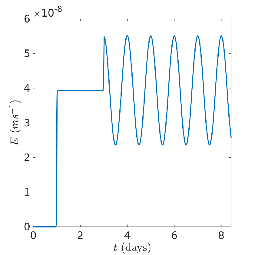
In order to test these observations on a concrete example, we consider a special time-varying transpiration source term as pictured in fig. 8a that begins at zero, jumps suddenly to a relatively large non-zero constant value (here ), and then after some delay returns to a “normal” diurnal periodic cycle (a pure mode). This source may be viewed physically as arising from a severe weather event or other rapid change in ambient conditions. To allow clear travelling waves to develop along the stem, we also concentrate the transpiration source term in a small region near the tree-top using the function as shown in fig. 8b.
| (a) | (b) | (c) |
 |
 |
 |
| (d) | (e) | (f) |
 |
 |
 |
Numerical simulations yield the time-dependent saturation profiles in fig. 8c at two different stem heights. In response to the initial transpiration jump, there is a clear relaxation phase where saturation decays gradually back to a constant steady state. The zoomed plot in fig. 8d shows that the relaxation time is roughly 3.5 h, which compares well with the estimate of h obtained using eq. 4.33, converted to dimensional time. Moving next to the diurnal variations in transpiration, the zoomed plot of the two saturation profiles in fig. 8e demonstrates the existence of travelling waves of saturation moving down the stem, shown as a time shift between the two corresponding peaks. The shift can be estimated as roughly h, whereas the asymptotic wave speed formula eq. 4.32 can be used to estimate a shift of h. A second simulation is shown for a larger value of in fig. 8f, which exhibits a computed shift of 2.7 h as compared with the asymptotic estimate of 2.86 h, which is a significantly better agreement.
One further verification of the asymptotic solution is now performed in which we compare the radially-averaged saturation profile from simulations to that obtained from the two-term asymptotic expansion over a one-day period. Taking so that , the relative difference between numerical and asymptotic values of the saturation deficit is . It is only when the transpiration rate is increased to that we begin to move out of the asymptotic regime and differences in saturation become visible to the naked eye as shown in fig. 9.
| (a) 3am to 2pm | (b) 2pm to 2am |
|---|---|
 |
 |
4.7 Discussion: Physical Relevance of Dimensionless Ratios
To conclude this section, we highlight four dimensionless parameters (or ratios) that play a prominent role in the asymptotic solution just derived, and which also have straightforward physical interpretations.
Stem aspect ratio,
This parameter plays a central role in the asymptotic analysis as the power series expansion parameter. One of our main conclusions is that the ratio of the radial and vertical velocity components is , which is small regardless of the conductivity ratio . Indeed, this is what allows us to assume in our asymptotic derivation and still obtain a solution whose leading order term is relevant to the anisotropic case.
Transpiration–flux ratio,
This ratio appears in several key places throughout the asymptotic derivation wherever transpiration terms appear in the solution, including eqs. 4.7, 4.17 and 4.26. Substituting the parameter definitions into yields
and based on the right-most expression may be interpreted as the ratio of transpiration flux through the stem surface to vertical sap flux through a circular stem cross-section. For the parameters of interest in this study , which reflects the balance that must exist between these two fluxes under “normal” daytime conditions. Other limits could nonetheless be considered, such as for which the transpiration rate is insufficient to generate an appreciable change in saturation and hence the impact of transpiration will only be felt in higher order terms. On the other hand, imposing a higher transpiration rate with could be viewed as shifting the tree into an embolism regime for which saturation is no longer a smooth function, violating a fundamental assumption in our model.
Gravity–saturation ratio,
This ratio also appears in the governing equations eqs. 4.4 and 4.12 and the leading order saturation boundary conditions eqs. 4.6 and 4.14. In terms of dimensional parameters, , which can be viewed as a balance between the driving force due to gravity, and the corresponding (saturation-dependent) capillary forces acting on the pore scale in both stem and roots. At night when transpiration is a minimum these two forces must be in balance to prevent water loss into the soil, which is reflected in the fact that . Recall that our analysis requires (when , see eq. 4.16) which places a restriction on the model parameters. For example, if tree height and radius are scaled up by the same factor so that remains fixed then the ratio must also increase, meaning that larger trees may develop larger tensions for a given saturation deficit.
Time parameter,
Consider the formulas for the travelling wave speed eq. 4.32 and relaxation time eq. 4.33 derived in the previous section. For simplicity, consider a tree with no taper () in which case the wave speed formula reduces to and the relaxation time to . Clearly, the parameter is intimately tied to the time variation of the solution both through the speed of propagation of saturation disturbances along the stem (with characteristic time proportional to ) and the time for decay of disturbances (proportional to ).
5 Conclusions
We have extended and generalized the 1D porous medium model for transpiration-driven tree sap flow developed by Chuang et al. in [7] to a tapered 3D axisymmetric stem geometry. Methods of asymptotic analysis are used to derive the first two terms in a regular asymptotic series expansion in powers of the aspect ratio , which are then used to obtain formulas for the spatial and temporal variations of the saturation and velocity components. Various possible flow regimes are studied through the use of several dimensionless ratios. The results are illustrated using a set of physical parameters and nonlinear coefficient functions corresponding to Norway spruce trees, although the analysis applies to a much more general class of parameters. One interesting conclusion of our analysis is that moderate levels of anisotropy in the hydraulic conductivity do not induce any radial flow (or radial solution dependence) at leading order so that the simpler isotropic porous medium solution is a reasonable approximation for moderate . Indeed, introducing an anisotropy that depends on powers has the effect of successively “shifting” radial variations up to the higher order terms in the asymptotic solution.
The asymptotic results are verified using a second order finite volume approximation of the original governing equations, showing the results to be accurate for a relatively large range of saturations (as long as we avoid the low pressure regime where embolisms are likely to form, at which point the model assumptions are no longer valid). An interesting correspondence is drawn between asymptotic results for the steady state case and the more pervasive circuit model representation for tree sap flow. Furthermore, the vertical mass flux was shown to agree with experimental results from [7].
In future, we plan to extend the model to a more general non-symmetric 3D geometry where the solution either experiences angular variations or a more complicated branching distribution along the stem. This model also forms an ideal platform from which to study the interplay between transpiration and embolism formation under more extreme conditions.
Our asymptotic analysis will also facilitate the study of inverse problems related to estimating the transpiration functions and , as well as model parameters such as , and . Given a set of noisy measurements of sap velocity, we can use our formulas to recover estimates of and . Then if is small enough that saturation relaxes to the zero transpiration steady-state at night, we may estimate using eq. 4.17. The parameter can then be determined using measurements of the relaxation time at night in eq. 4.33. Finally, assuming that data for is available from vulnerability curve measurements, can be estimated making use of values for and . The details of this estimation procedure can be found in [16].
References
- [1] G. Angeles et al., The cohesion-tension theory, New Phytologist, 163 (2004), pp. 451–452.
- [2] C. A. Aumann and E. D. Ford, Modeling tree water flow as an unsaturated flow through a porous medium, Journal of Theoretical Biology, 219 (2002), pp. 415–429.
- [3] , Parameterizing a model of Douglas fir water flow using a tracheid-level model, Journal of Theoretical Biology, 219 (2002), pp. 431–462.
- [4] G. Bohrer, H. Mourad, T. A. Laursen, D. Drewry, R. Avissar, D. Poggi, R. Oren, and G. G. Katul, Finite element tree crown hydrodynamics model (FETCH) using porous media flow within branching elements: A new representation of tree hydrodynamics, Water Resources Research, 41 (2005), p. W11404.
- [5] C. Brodersen and A. McElrone, Maintenance of xylem network transport capacity: A review of embolism repair in vascular plants, Frontiers in Plant Science, 4 (2013), p. 108.
- [6] H. R. Brown, The theory of the rise of sap in trees: Some historical and conceptual remarks, Physics in Perspective, 15 (2013), pp. 320–358.
- [7] Y.-L. Chuang, R. Oren, A. L. Bertozzi, N. Phillips, and G. G. Katul, The porous media model for the hydraulic system of a conifer tree: Linking sap flux data to transpiration rate, Ecological Modelling, 191 (2006), pp. 447–468.
- [8] G. L. Comstock, Directional permeability of softwoods, Wood and Fiber, 1 (1970), pp. 283–289.
- [9] I. R. Cowan, Transport of water in the soil-plant-atmosphere system, Journal of Applied Ecology, 2 (1965), pp. 221–239.
- [10] P. Cruiziat, H. Cochard, and T. Améglio, Hydraulic architecture of trees: Main concepts and results, Annals of Forest Science, 59 (2002), pp. 723–752.
- [11] H. H. Dixon and J. Joly, On the ascent of sap, Annals of Botany, 8 (1894), pp. 468–470.
- [12] J.-C. Domec, F. C. Meinzer, B. L. Gartner, and D. Woodruff, Transpiration-induced axial and radial tension gradients in trunks of Douglas-fir trees, Tree Physiology, 26 (2006), pp. 275–284.
- [13] T. Früh and W. Kurth, The hydraulic system of trees: Theoretical framework and numerical simulation, Journal of Theoretical Biology, 201 (1999), pp. 251–270.
- [14] E. R. Hunt and P. S. Nobel, Non-steady-state water flow for three desert perennials with different capacitances, Functional Plant Biology, 14 (1987), pp. 363–375.
- [15] S. A. James, F. C. Meinzer, G. Goldstein, D. Woodruff, T. Jones, T. Restom, M. Mejia, M. Clearwater, and P. Campanello, Axial and radial water transport and internal water storage in tropical forest canopy trees, Oecologia, 134 (2003), pp. 37–45.
- [16] B. M. Janbek, Mathematical Modelling of Sap Flow and Heat Transport in Trees, PhD thesis, Department of Mathematics, Simon Fraser University, Burnaby, Canada, summer 2017.
- [17] K. H. Jensen, K. Berg-Sørensen, H. Bruus, N. M. Holbrook, J. Liesche, A. Schulz, M. A. Zwieniecki, and T. Bohr, Sap flow and sugar transport in plants, Reviews of Modern Physics, 88 (2016), p. 035007.
- [18] W. Kang and W. Y. Chung, Liquid water diffusivity of wood from the capillary pressure–moisture relation, Journal of Wood Science, 55 (2009), pp. 91–99.
- [19] J. Kevorkian and J. D. Cole, Perturbation Methods in Applied Mathematics, Springer-Verlag, New York, NY, 1981.
- [20] A. Klute, A numerical method for solving the flow equation for water in unsaturated materials, Soil Science, 73 (1952), pp. 105–116.
- [21] T. Kumagai, Modeling water transportation and storage in sapwood – model development and validation, Agricultural and Forest Meteorology, 109 (2001), pp. 105–115.
- [22] R. Li and A. R. Weiskittel, Comparison of model forms for estimating stem taper and volume in the primary conifer species of the North American Acadian Region, Annals of Forest Science, 67 (2010), p. 302.
- [23] P. Lu, P. Biron, A. Granier, and H. Cochard, Water relations of adult Norway spruce (Picea abies (L) Karst) under soil drought in the Vosges mountains: Water potential, stomatal conductance and transpiration, Annales des Sciences Forestières, 53 (1996), pp. 113–121.
- [24] K. J. Niklas, Size-dependent allometry of tree height, diameter and trunk-taper, Annals of Botany, 75 (1995), pp. 217–227.
- [25] M. Perämäki, T. Vesala, and E. Nikinmaa, Modeling the dynamics of pressure propagation and diameter variation in tree sapwood, Tree Physiology, 25 (2005), pp. 1091–1099.
- [26] N. Phillips, A. Nagchaudhuri, R. Oren, and G. Katul, Time constant for water transport in loblolly pine trees estimated from time series of evaporative demand and stem sapflow, Trees, 11 (1997), pp. 412–419.
- [27] W. F. Pickard, The ascent of sap in plants, Progress in Biophysics and Molecular Biology, 37 (1981), pp. 181–229.
- [28] R. Poyatos, J. Čermák, and P. Llorens, Variation in the radial patterns of sap flux density in pubescent oak (Quercus pubescens) and its implications for tree and stand transpiration measurements, Tree Physiology, 27 (2007), pp. 537–548.
- [29] A. L. Redman, H. Bailleres, I. Turner, and P. Perré, Mass transfer properties (permeability and mass diffusivity) of four Australian hardwood species, BioResources, 7 (2012), pp. 3410–3424.
- [30] D. E. B. Reid, U. Silins, C. Mendoza, and V. J. Lieffers, A unified nomenclature for quantification and description of water conducting properties of sapwood xylem based on Darcy’s law, Tree Physiology, 25 (2005), pp. 993–1000.
- [31] A. Sellin, Sapwood-heartwood proportion related to tree diameter, age, and growth rate in Picea abies, Canadian Journal of Forest Research, 24 (1994), pp. 1022–1028.
- [32] K. Steppe, D. J. W. De Pauw, R. Lemeur, and P. A. Vanrolleghem, A mathematical model linking tree sap flow dynamics to daily stem diameter fluctuations and radial stem growth, Tree Physiology, 26 (2006), pp. 257–273.
- [33] A. Szymkiewicz, Modelling Water Flow in Unsaturated Porous Media, GeoPlanet: Earth and Planetary Sciences, Springer-Verlag, Berlin, 2013.
- [34] L. Taiz and E. Zeiger, Plant Physiology, Sinaeur Associates Inc., Sunderland, MA, third ed., 2002.
- [35] L. Testi and F. J. Villalobos, New approach for measuring low sap velocities in trees, Agricultural and Forest Meteorology, 149 (2009), pp. 730–734.
- [36] M. T. Tyree, A dynamic model for water flow in a single tree: Evidence that models must account for hydraulic architecture, Tree Physiology, 4 (1988), pp. 195–217.
- [37] T. H. Van den Honert, Water transport in plants as a catenary process, Discussions of the Faraday Society, 3 (1948), pp. 146–153.
- [38] S. D. Wullschleger and A. W. King, Radial variation in sap velocity as a function of stem diameter and sapwood thickness in yellow-poplar trees, Tree Physiology, 20 (2000), pp. 511–518.
- [39] M. H. Zimmermann, Xylem Structure and the Ascent of Sap, Springer-Verlag, New York, NY, 1983.