Moving Mesh Finite Element Simulation for Phase-Field Modeling of Brittle Fracture and Convergence of Newton’s Iteration

We first describe small strain isotropic elasticity models without cracks. We consider an elastic body occupying a bounded domain $\Omega\subset\mathbb{R}^{2}$ with the boundary $\partial\Omega=\partial\Omega_{t}\cup\partial\Omega_{u}$, where the surface traction $\overline{t}$ is specified on $\partial\Omega_{t}$ and the displacement $\overline{u}$ is given on $\partial\Omega_{u}$. The strain tensor is given by

$$\epsilon=\frac{1}{2}\left(\nabla u+(\nabla u)^{T}\right),$$

where $\nabla{u}$ is the displacement gradient tensor. For isotropic material without damage, the elastic energy per unit volume, or strain energy density, is given by Hooke’s law as

$$W_{e}(\epsilon)=\frac{\lambda}{2}\left(\tr({\epsilon})\right)^{2}+\mu\tr({\epsilon}^{2}),$$

(1)

where $\lambda$ and $\mu$ are the Lamé constants. The stress tensor is given by the derivative of the strain energy with respect to the strain tensor, i.e.,

$$\sigma:=\frac{\partial W_{e}}{\partial{\epsilon}}=\lambda\tr({\epsilon})I+2\mu{\epsilon},$$

(2)

where the symbol $:=$ stands for “definition”. Then the total strain energy stored in the elastic solid is given by

$$\mathcal{W}_{e}({\epsilon})=\int_{\Omega}W_{e}({\epsilon})\,d\Omega.$$

(3)

The variation of $\mathcal{W}_{e}$ is

$$\delta\mathcal{W}_{e}=\int_{\Omega}\frac{\partial W_{e}}{\partial\epsilon}:\delta\epsilon\,d\Omega=\int_{\Omega}\sigma:\epsilon(\delta u)\,d\Omega,$$

(4)

where $A:B$ is the inner product of tensors $A$ and $B$, i.e., $A:B=\sum\limits_{i,j}A_{i,j}B_{i,j}$. Define the function spaces

	$$\displaystyle V_{u}=\left\{\;\varphi\;|\;\varphi\in H^{1}(\Omega),\;\varphi=\overline{u}\;\text{on}\;\partial\Omega_{u}\right\},$$
	$$\displaystyle V_{u}^{0}=\left\{\;\varphi\;|\;\varphi\in H^{1}(\Omega),\;\varphi=0\;\text{on}\;\partial\Omega_{u}\right\},$$

where $H^{1}(\Omega)$ is a Sobolev space, viz.,

$$H^{1}(\Omega)=\left\{\;\varphi\;|\;\int_{\Omega}\varphi^{2}\,d\Omega<+\infty,\;\int_{\Omega}(\nabla\varphi)^{2}\,d\Omega<+\infty\right\}.$$

If we add the boundary traction $\overline{t}$ and body force $f$, then the variational formulation of the elasticity model is to find $u\in V_{u}$ such that

$$\int_{\Omega}\sigma:{\epsilon}(\delta{u})\,d\Omega=\int_{\partial\Omega_{t}}\overline{t}\cdot\delta{u}\,dS+\int_{\Omega}f\cdot\delta{u}\,d\Omega,\quad\forall\;\delta u\in V_{u}^{0}.$$

(5)

We now consider the situation with cracks in the elastic body. We use the approach proposed by Francfort and Marigo [17] where the total energy of the body with a given crack $\Gamma$ is given by

$$\mathcal{W}({\epsilon},\Gamma)=\mathcal{W}_{e}({\epsilon},\Gamma)+\mathcal{W}_{c}(\Gamma):=\int_{\Omega\setminus\Gamma}W_{e}({\epsilon},\Gamma)\,d\Omega+\int_{\Gamma}g_{c}\,dS,$$

where $\mathcal{W}_{e}({\epsilon},\Gamma)$ represents the energy stored in the bulk of the elastic body, $\mathcal{W}_{c}(\Gamma)$ is the energy required to create the crack according to the Griffith criterion, and $g_{c}$ is the fracture energy density (also referred to as the fracture toughness) which is the amount of energy needed to create a unit area of fracture surface.

In the phase-field modeling, the fracture surface is approximated by a phase-field variable $d(x,t)$, which depends on a parameter $l$ describing the width of the smooth approximation of the crack. This function is smooth with the value 0 or close to 0 near the crack and 1 away from the crack (see Fig. 1). The fracture energy $\mathcal{W}_{c}(\Gamma)$ is approximated by the smeared total fracture energy [13] as

$$\mathcal{W}_{c}^{l}=\int_{\Omega}\frac{g_{c}}{4l}\left((d-1)^{2}+4l^{2}|\nabla d|^{2}\right)d\Omega.$$

(6)

The elastic energy $\mathcal{W}_{e}({\epsilon},\Gamma)$ needs to be modified to reflect the loss of material stiffness in the damage zone. We follow the approach by Miehe et al. [40]. Define the decomposition of a scalar function $f$ as

$$f=f^{+}+f^{-},\quad f^{+}=\frac{f+|f|}{2},\quad f^{-}=\frac{f-|f|}{2}.$$

Assuming that the strain tensor has the eigen-decomposition $\epsilon=Q\text{diag}(\lambda_{1},...,\lambda_{n})Q^{T}$, we define

$$\epsilon=\epsilon^{+}+\epsilon^{-},\quad\epsilon^{+}=Q\text{diag}(\lambda_{1}^{+},...,\lambda_{n}^{+})Q^{T},\quad\epsilon^{-}=Q\text{diag}(\lambda_{1}^{-},...,\lambda_{n}^{-})Q^{T}.$$

(7)

The tensile strain component, $\epsilon^{+}$, contributes to the damage process resulting in crack initiation and propagation whereas the compression strain component, $\epsilon^{-}$, does not contribute to the damage process. A commonly used damage model is given as

$$W_{e}=g(d)\Psi^{+}(\epsilon)+\Psi^{-}(\epsilon),$$

(8)

where $g(d)$ is a degradation function that describes the reduction of the stiffness of the bulk of the solid and

$$\Psi^{+}(\epsilon)=\frac{\lambda}{2}\left((\tr(\epsilon))^{+}\right)^{2}+\mu\tr((\epsilon^{+})^{2}),\quad\Psi^{-}(\epsilon)=\frac{\lambda}{2}\left((\tr(\epsilon))^{-}\right)^{2}+\mu\tr((\epsilon^{-})^{2}).$$

The degradation function $g(d)$ is required to satisfy the property (e.g., see [33])

$$\begin{cases}g(0)=0:&\quad\text{Damage occurred for $d=0$ and this part should vanish};\\ g(1)=1:&\quad\text{No damage occurs for $d=1$};\\ g^{\prime}(0)=0:&\quad\text{No more changes after the fully broken state};\\ g^{\prime}(1)\neq 0:&\quad\text{The damage has to be initiated at the onset.}\end{cases}$$

We take a commonly used quadratic degradation function $g(d)=d^{2}$ in our computation. Combining (6) and (8), we obtain the total energy as

$$\mathcal{W}^{l}=\mathcal{W}_{e}+\mathcal{W}_{c}^{l}=\int_{\Omega}\left((d^{2}+k_{l})\Psi^{+}(\epsilon)+\Psi^{-}(\epsilon)+\frac{g_{c}}{4l}\left((d-1)^{2}+4l^{2}|\nabla d|^{2}\right)\right)d\Omega,$$

(9)

where $k_{l}\ll l$ is the (small) regularization parameter for avoiding degeneracy. The variation of the energy is

$$\delta\mathcal{W}^{l}=\int_{\Omega}\frac{\partial W}{\partial d}\delta d\;d\Omega+\int_{\Omega}\frac{\partial W}{\partial\nabla d}\cdot\nabla\delta d\;d\Omega+\int_{\Omega}\frac{\partial W}{\partial\epsilon}:\epsilon(\delta u)\;d\Omega$$

where

$$W=(d^{2}+k_{l})\Psi^{+}(\epsilon)+\Psi^{-}(\epsilon)+\frac{g_{c}}{4l}\left((d-1)^{2}+4l^{2}|\nabla d|^{2}\right).$$

The weak formulation is to find $d\in V_{d}=H^{1}(\Omega)$ (with $d$ satisfying a homogeneous Neumann boundary condition) and $u\in V_{u}$ such that

		$\displaystyle\int_{\Omega}\left(\left(2d\mathcal{H}+\frac{g_{c}(d-1)}{2l}\right)\delta d+2g_{c}l\nabla d\cdot\nabla\delta d\right)d\Omega=0,\quad\forall\;\delta d\in V_{d}$		(10)
		$\displaystyle\int_{\Omega}\sigma:\epsilon(\delta u)d\Omega=\int_{\Omega_{t}}\overline{t}\cdot\delta{u}\;dS+\int_{\Omega}f\cdot\delta{u}\;d\Omega,\quad\forall\;\delta u\in V_{u}^{0}$		(11)

where $\mathcal{H}=\Psi^{+}(\epsilon)$ and

$$\sigma:=\frac{\partial W}{\partial\epsilon}=(d^{2}+k_{l})\left(\lambda(\tr(\epsilon))^{+}I+2\mu\epsilon^{+}\right)+\left(\lambda(\tr(\epsilon))^{-}I+2\mu\epsilon^{-}\right).$$

(12)

To ensure crack irreversibility in the sense that the cracks can only grow, we replace $\mathcal{H}=\Psi^{+}(\epsilon)$ in (10) by

$$\mathcal{H}=\max_{s\leq t}\Psi^{+}(\epsilon)(s),$$

(13)

where $t$ is the quasi-time corresponding to the load increments.

In addition to the above described decomposition by Miehe et al. [40], there is another often-used decomposition by Amor et al. [3] that is based on the split of the strain tensor into volumetric and deviatoric parts. Discussion of the advantages and disadvantages of both decompositions can be found in [1, 9].

We consider a simplicial mesh $\mathcal{T}_{h}$ for the domain $\Omega$ and denote the number of its elements and vertices by $N$ and $N_{v}$, respectively. The piecewise linear approximations of the function spaces $V_{d}$, $V_{u}$ and $V_{u}^{0}$ are given by

		$\displaystyle V_{d}^{h}=\left\{\varphi_{h}\;|\;\varphi_{h}\in C^{0}(\overline{\Omega})\cap V_{d};\;\varphi_{h}|_{K}\in P_{1}(K),\;\forall K\in\mathcal{T}_{h}(\Omega)\right\},$
		$\displaystyle V_{u}^{h}=\left\{\varphi_{h}\;|\;\varphi_{h}\in C^{0}(\overline{\Omega})\cap V_{u};\;\varphi_{h}|_{K}\in P_{1}(K),\;\forall K\in\mathcal{T}_{h}(\Omega)\right\},$
		$\displaystyle V_{u}^{0,h}=\left\{\varphi_{h}\;|\;\varphi_{h}\in C^{0}(\overline{\Omega})\cap V_{u}^{0};\;\varphi_{h}|_{K}\in P_{1}(K),\;\forall K\in\mathcal{T}_{h}(\Omega)\right\},$

where $P_{1}(K)$ is the set of polynomials of degree less than or equal to 1 defined on $K$. The linear finite element approximation of the phase-field problem (10) and (11) is to find $d_{h}\in V_{d}^{h}$ and $u_{h}\in V_{u}^{h}$ such that

		$\displaystyle\int_{\Omega}\left(\left(2d_{h}\mathcal{H}+\frac{g_{c}(d_{h}-1)}{2l}\right)\varphi_{h}+2g_{c}l\nabla d_{h}\cdot\nabla\varphi_{h}\right)d\Omega=0,\quad\forall\;\varphi_{h}\in V_{d}^{h}$		(14)
		$\displaystyle\int_{\Omega}\sigma(u_{h}):\epsilon(\varphi_{h})d\Omega=\int_{\Omega_{t}}\overline{t}\cdot\varphi_{h}\;dS+\int_{\Omega}f\cdot\varphi_{h}\;d\Omega,\quad\forall\;\varphi_{h}\in V_{u}^{0,h}.$		(15)

Note that $u_{h}$ and $d_{h}$ are strongly coupled through (14) and (15). Common procedures for solving these equations can be roughly categorized into two groups, simultaneous (or called monolithic) solution and alternating (or called staggered) solution. In the former group (such as see [19, 20, 57, 58]) the phase-field variable and displacement are solved simultaneously often by Newton’s method. This procedure has to deal with a large system and the highly nonlinear coupling between $d_{h}$ and $u_{h}$. Moreover, the decomposition of the strain tensor further increases the nonlinearity (see Section 3.2 for detailed discussion). It is still challenging to obtain a convergent solution using the simultaneous solution procedure. The second solution procedure (such as see [1, 3, 40, 42]) is to solve (14) for $d_{h}$ and (15) for $u_{h}$ alternatingly. One of the advantages of this approach is that $d_{h}$ and $u_{h}$ are not coupled. Moreover, (14) is linear about $d_{h}$ and its solution does not need Newton’s iteration.

In our computation, we use the alternating solution procedure and consider the problem in a quasi-static condition. The quasi-time $t$ is introduced to represent the load increments. The solution procedure from $t^{n}$ to $t^{n+1}$ is described as follows.

1. (i)

   We assume that the mesh $\mathcal{T}_{h}^{n}$ at time $t^{n}$ and the history field $\mathcal{H}_{h}^{n}$ in (13) (defined on $\mathcal{T}_{h}^{n}$) are given.

2. (ii)

   Compute the phase-field variable $d_{h}^{n+1}$ and new mesh $\mathcal{T}_{h}^{n+1}$ as follows.

   • •

     Set $\mathcal{T}_{h}^{n+1,1}=\mathcal{T}_{h}^{n}$;

   • •

     For $k=1:kk$

     • -

       Compute $\mathcal{H}$ on $\mathcal{T}_{h}^{n+1,k}$ using linear interpolation of $\mathcal{H}_{h}^{n}$;

     • -

       Compute $d_{h}^{n+1,k}$ using (14) and $\mathcal{H}$ on $\mathcal{T}_{h}^{n+1,k}$;

     • -

       If $k<kk$, compute the new mesh $\mathcal{T}_{h}^{n+1,k+1}$ by the MMPDE moving mesh method based on $\mathcal{T}_{h}^{n+1,k}$ and $d_{h}^{n+1,k}$. (See Section 3.3)

   • •

     Set $\mathcal{T}_{h}^{n+1}=\mathcal{T}_{h}^{n+1,kk}$ and $d_{h}^{n+1}=d_{h}^{n+1,kk}$.

3. (iii)

   Compute the displacement field $u_{h}^{n+1}$ by solving the nonlinear system (15) based on $d_{h}^{n+1}$ and $\mathcal{T}_{h}^{n+1}$. (See Section 3.2)

4. (iv)

   Compute $\Psi^{+,n+1}_{h}(\epsilon(u_{h}^{n+1}))$ and interpolate $\mathcal{H}_{h}^{n}$ from the old mesh $\mathcal{T}_{h}^{n}$ to the new mesh $\mathcal{T}_{h}^{n+1}$ using linear interpolation and denote it by $\tilde{\mathcal{H}}_{h}^{n+1}$. Let $\mathcal{H}_{h}^{n+1}=\max\{\Psi^{+,n+1}_{h}(\epsilon(u_{h}^{n+1})),\tilde{\mathcal{H}}_{h}^{n+1}\}$.

In the above procedure, the parameter $kk$ can affect the adaptivity of the mesh $\mathcal{T}_{h}^{n+1}$ to the phase-field variable $d_{h}^{n+1}$. From our computational experience, we choose $kk=5$, for which we have found that $\mathcal{T}_{h}^{n+1}$ is sufficiently adaptive to $d_{h}^{n+1}$ but without compromising the computational efficiency too much.

We recall that the strain tensor is decomposed into tensile and compressive components (cf. (7)), with only the former component contributing to generation of cracks. The tensile and compressive components are nonsmooth functions of the displacement, which has two major effects on Newton’s iteration applied to the solution of the equation (15), the existence and computation of the Jacobian matrix and the convergence of Newton’s iteration. As can be seen in Fig. 2(a) and Fig. 2(b), the Jacobian matrix of equation (15) does not exist in the places where any of the eigenvalues vanishes. In other places where the eigenvalues do not vanish, the computation of the Jacobian matrix can also be tricky. In principle, the analytical expressions of the derivatives of $\epsilon^{+}$ and $\epsilon^{-}$ with respect to $\epsilon$ can be obtained through the derivatives of the eigenvalues and eigenvectors with respect to $\epsilon$ (e.g, see [37]). However, these expressions are too complicated to be used in practical computation. Special algorithms are needed to compute these derivatives using analytical formulas; see Miehe [39] and Miehe and Lambrecht [41].

Another effect of the decomposition of the strain tensor is that Newton’s iteration often fails to converge; see the numerical examples in Section 4.1.1. The degeneracy of the equation (15) can further complicate the situation. In principle, the regularization parameter $k_{l}$ can be chosen sufficiently large to make Newton’s iteration to converge. However, a large value of $k_{l}$ will smear the crack and lead to an unphysically overestimated bulk energy.

To overcome the above mentioned difficulties, we propose to smooth out the decomposition (7) and compute the Jacobian matrix of the equation (15) using finite differences. The latter is straightforward so we will not elaborate it here. For the former, there are a variety of regularization methods. We consider here three of these methods where the positive and negative eigenvalue functions are smoothed using a switching technique or convolution with a smoothed delta function (or a mollifier).

• •

  The sonic-point regularization method. We first consider the so-called eigenvalue-switching technique which is used to obtain a smooth transition of the solution through the sonic point [4] in computational fluid dynamics. The regularized positive and negative eigenvalue functions are defined as

  $$\lambda_{\alpha}^{+}=\frac{\lambda+\sqrt{\lambda^{2}+\alpha^{2}}}{2},\quad\lambda_{\alpha}^{-}=\frac{\lambda-\sqrt{\lambda^{2}+\alpha^{2}}}{2},$$

  where $\alpha>0$ is the regularization parameter.

• •

  The exponential convolution method. The second regularization method is to take the convolution of $\lambda^{+}$ and $\lambda^{-}$ with the exponential delta function

  $$\delta_{\alpha}(\lambda)=\frac{1}{\sqrt{2\pi}\alpha}e^{-\frac{\lambda^{2}}{2\alpha^{2}}}.$$

  Then the regularized positive and negative eigenvalue functions are given by

  		$\displaystyle\lambda_{\alpha}^{+}=\int_{-\infty}^{\infty}\lambda^{+}(\eta)\delta_{\alpha}(\lambda-\eta)d\eta=\frac{\lambda}{2}\left(1+\text{erf}\left(\frac{\lambda}{\sqrt{2}\alpha}\right)\right)+\frac{\alpha}{\sqrt{2\pi}}e^{-\frac{\lambda^{2}}{2\alpha^{2}}},$
  		$\displaystyle\lambda_{\alpha}^{-}=\int_{-\infty}^{\infty}\lambda^{-}(\eta)\delta_{\alpha}(\lambda-\eta)d\eta=\frac{\lambda}{2}\left(1+\text{erf}\left(-\frac{\lambda}{\sqrt{2}\alpha}\right)\right)-\frac{\alpha}{\sqrt{2\pi}}e^{-\frac{\lambda^{2}}{2\alpha^{2}}}.$

• •

  The smoothed 2-point convolution method. The third method is similar to the exponential convolution method but with a localized, smoothed 2-point delta function

  $$\delta_{\alpha}(\lambda)=\begin{cases}\frac{1}{\alpha}\left(\frac{3}{4}-\frac{\lambda^{2}}{\alpha^{2}}\right),\quad&\text{ for }|\lambda|\leqslant 0.5\alpha\\ \frac{1}{\alpha}\left(\frac{9}{8}-\frac{3}{2}\frac{|\lambda|}{\alpha}+\frac{1}{2}\frac{\lambda^{2}}{\alpha^{2}}\right),\quad&\text{ for }0.5\alpha\leqslant|\lambda|\leqslant 1.5\alpha\\ 0,\quad&\text{ for }|\lambda|\geqslant 1.5\alpha.\end{cases}$$

  We then have

  		$\displaystyle\lambda_{\alpha}^{+}=\begin{cases}0,\quad&\text{ for }\lambda\leqslant-1.5\alpha\\ \frac{1}{\alpha}\left(\frac{1}{24\alpha^{2}}\lambda^{4}+\frac{1}{4\alpha}\lambda^{3}+\frac{9}{16}\lambda^{2}+\frac{9\alpha}{16}\lambda+\frac{27\alpha^{2}}{128}\right),\quad&\text{ for }-1.5\alpha\leqslant\lambda\leqslant-0.5\alpha\\ \frac{1}{\alpha}\left(-\frac{1}{12\alpha^{2}}\lambda^{4}+\frac{3}{8}\lambda^{2}+\frac{\alpha}{2}\lambda+\frac{13\alpha^{2}}{64}\right),\quad&\text{ for }-0.5\alpha\leqslant\lambda\leqslant 0.5\alpha\\ \frac{1}{\alpha}\left(\frac{1}{24\alpha^{2}}\lambda^{4}-\frac{1}{4\alpha}\lambda^{3}+\frac{9}{16}\lambda^{2}+\frac{7\alpha}{16}\lambda+\frac{27\alpha^{2}}{128}\right),\quad&\text{ for }0.5\alpha\leqslant\lambda\leqslant 1.5\alpha\\ \lambda,\quad&\text{ for }\lambda\geqslant 1.5\alpha\end{cases}$
  		$\displaystyle\lambda_{\alpha}^{-}=\begin{cases}\lambda,\quad&\text{ for }\lambda\leqslant-1.5\alpha\\ \frac{1}{\alpha}\left(-\frac{1}{24\alpha^{2}}\lambda^{4}-\frac{1}{4\alpha}\lambda^{3}-\frac{9}{16}\lambda^{2}+\frac{7\alpha}{16}\lambda-\frac{27\alpha^{2}}{128}\right),\quad&\text{ for }-1.5\alpha\leqslant\lambda\leqslant-0.5\alpha\\ \frac{1}{\alpha}\left(\frac{1}{12\alpha^{2}}\lambda^{4}-\frac{3}{8}\lambda^{2}+\frac{\alpha}{2}\lambda-\frac{13\alpha^{2}}{64}\right),\quad&\text{ for }-0.5\alpha\leqslant\lambda\leqslant 0.5\alpha\\ \frac{1}{\alpha}\left(-\frac{1}{24\alpha^{2}}\lambda^{4}+\frac{1}{4\alpha}\lambda^{3}-\frac{9}{16}\lambda^{2}+\frac{9\alpha}{16}\lambda-\frac{27\alpha^{2}}{128}\right),\quad&\text{ for }0.5\alpha\leqslant\lambda\leqslant 1.5\alpha\\ 0,\quad&\text{ for }\lambda\geqslant 1.5\alpha.\end{cases}$

It is remarked that all of the above regularization methods satisfy

$$\lambda=\lambda^{+}_{\alpha}+\lambda^{-}_{\alpha}$$

(16)

and thus

$$\epsilon=\epsilon_{\alpha}^{+}+\epsilon_{\alpha}^{-}.$$

(17)

Moreover, as can be seen in Fig. 2(c), all of the methods provide a smooth transition around zero for both positive and negative eigenvalue functions. Furthermore, the sonic-point and exponential convolution methods have global effects whereas the smoothed 2-point convolution method only changes the values near $\lambda=0$. Finally, for a fixed value of the regularization parameter, $\alpha=3\times 10^{-3}$, in terms of the closeness of the curve of $\lambda_{\alpha}^{+}$ ($\lambda_{\alpha}^{-}$) to that of $\lambda^{+}$ (or $\lambda^{-}$) the best is the smoothed 2-point convolution and then the exponential convolution and sonic-point methods.

The effects of these regularization methods on the the convergence of Newton’s iteration and on the numerical solution will be discussed in Section 4.1.1. It is worth mentioning that we have tried a few other regularization methods which only modify the local behavior of the eigenvalue function near the origin. Since they do not satisfy (16) in general and are much less effective in making Newton’s iteration convergent than the above methods, we choose not to report them here to save space.

In this section we describe the MMPDE moving mesh method [26, 28] for generating the new mesh $\mathcal{T}_{h}^{n+1}$ (as mentioned in Section 3.1). The method takes the $\mathbb{M}$-uniform mesh approach where a nonuniform mesh is viewed as a uniform one in the metric specified by a tensor $\mathbb{M}$. In our computation, we choose the metric tensor as

$$\mathbb{M}=\det(I+|H(d_{h})|)^{-\frac{1}{6}}(I+|H(d_{h})|),$$

(18)

where $H(d_{h})$ is a recovered Hessian of $d_{h}$ and $|H(d_{h})|=Q\text{diag}(|\lambda_{1}|,...,|\lambda_{2}|)Q^{T}$, assuming that the eigen-decomposition of $H(d_{h})$ is $Q\text{diag}(\lambda_{1},...,\lambda_{2})Q^{T}$. The recovered Hessian of $d_{h}$ at a vertex is obtained by twice differentiating a local quadratic polynomial fitting in the least-squares sense to the nodal values of $d_{h}$ at the neighboring vertices. The form of (18) is known optimal in terms of the $L^{2}$ norm of linear interpolation error on triangular meshes (e.g., see [29]). Notice that $\mathbb{M}$ is symmetric and uniformly positive define on $\Omega$. It will be used to control the shape, size, and orientation of mesh elements through the so-called equidistribution and alignment conditions (to be discussed below). Since (18) is based on the Hessian of the phase-field variable $d$, we may expect that the mesh elements are concentrated in the crack regions where the curvature of $d$ is large.

Let $x_{1},....,x_{N_{v}}$ be the coordinates of the vertices of $\mathcal{T}_{h}$. We choose the very initial physical (simplicial) mesh as the reference computational mesh which is denoted by $\hat{\mathcal{T}}_{c,h}=\{\hat{\xi}_{1},...,\hat{\xi}_{N_{v}}\}$. For the purpose of mesh generation, we need an intermediate simplicial mesh which we refer to as a computational mesh, $\mathcal{T}_{c,h}=\{\xi_{1},...,\xi_{N_{v}}\}$. We assume that $\mathcal{T}_{h}$, $\hat{\mathcal{T}}_{c,h}$, and $\mathcal{T}_{c,h}$ have the same number of elements and vertices and the same connectivity. As a consequence, there exists a unique element $K_{c}\in\mathcal{T}_{c,h}$ corresponding to any element $K\in\mathcal{T}_{h}$. The affine mapping between $K_{c}$ and $K$ is denoted by $F_{K}$ and its Jacobian matrix by $F_{K}^{\prime}$. Let the coordinates of the vertices of $K$ and $K_{c}$ be $x_{0}^{K},\,x_{1}^{K},\,x_{2}^{K}$ and $\xi_{0}^{K},\,\xi_{1}^{K},\,\xi_{2}^{K}$, respectively. Then we have

	$$\displaystyle F_{K}(\xi_{i}^{K})=x_{i}^{K},\quad i=0,1,2$$
	$$\displaystyle F^{\prime}_{K}(\xi_{i}^{K}-\xi_{0}^{K})=x_{i}^{K}-x_{0}^{K},\quad i=1,2.$$

From this we get

$$F^{\prime}_{K}=E_{K}\hat{E_{K}}^{-1},\quad(F^{\prime}_{K})^{-1}=\hat{E_{K}}E_{K}^{-1},$$

where $E_{K}$ and $\hat{E}_{K}$ are the edge matrices of $K$ and $K_{c}$ defined as

$$E_{K}=[x_{1}^{K}-x_{0}^{K},x_{2}^{K}-x_{0}^{K}],\quad\hat{E}_{K}=[\xi_{1}^{K}-\xi_{0}^{K},\xi_{2}^{K}-\xi_{0}^{K}].$$

The objective of the MMPDE moving mesh method is to generate an adaptive mesh as a uniform one in the metric $\mathbb{M}$. Such an $\mathbb{M}$-uniform mesh requires that (i) the ratio of the area of $K$ in the metric $\mathbb{M}$ to the area of $K_{c}$ in the Euclidean metric stay constant for all elements and (ii) $K$ measured in the metric $\mathbb{M}$ be similar to $K_{c}$ measured in the Euclidean metric for all elements. These two requirements can be expressed mathematically as the equidistribution and alignment conditions (e.g., see [23, 28]),

		$\displaystyle|K|\sqrt{\det(\mathbb{M}_{K})}=\frac{|\Omega_{h}|\;|K_{c}|}{|\Omega_{c}|},\quad\forall{K}\in\mathcal{T}_{h}$		(19)
		$\displaystyle\frac{1}{2}\tr\left((F^{\prime}_{K})^{T}\mathbb{M}_{K}F^{\prime}_{K}\right)=\det\left((F^{\prime}_{K})^{T}\mathbb{M}_{K}F^{\prime}_{K}\right)^{\frac{1}{2}},\quad K\in\mathcal{T}_{h}$		(20)

where $|K|$ and $|K_{c}|$ denote the area of $K$ and $K_{c}$, respectively, $\mathbb{M}_{K}$ is the average of $\mathbb{M}$ over $K$, $\det(\cdot)$ and $\tr(\cdot)$ denote the determinant and trace of a matrix, and

$$|\Omega_{h}|=\sum_{K\in\mathcal{T}_{h}}|K|\sqrt{\det(\mathbb{M}_{K})},\quad|\Omega_{c}|=\sum_{K_{c}\in\mathcal{T}_{c,h}}|K_{c}|.$$

An energy functional based on these conditions has been proposed by Huang [21] as

$$I_{h}(\mathcal{T}_{h};\mathcal{T}_{c,h})=\sum_{K\in\mathcal{T}_{h}}|K|G(\mathbb{J}_{K},\det(\mathbb{J}_{K}),\mathbb{M}_{K}),$$

(21)

where $\mathbb{J}_{K}=(F^{\prime}_{K})^{-1}$ and

	$\displaystyle G(\mathbb{J}_{K},\det(\mathbb{J}_{K}),\mathbb{M}_{K})$	$\displaystyle=\theta\sqrt{\det(\mathbb{M}_{K})}\left(\tr(\mathbb{J}_{K}\mathbb{M}_{K}\mathbb{J}^{T}_{K})\right)^{p}$
		$\displaystyle+(1-2\theta)2^{p}\sqrt{\det(\mathbb{M}_{K})}\left(\frac{\det(\mathbb{J}_{K})}{\sqrt{\det(\mathbb{M}_{K})}}\right)^{p}.$

Here, $0<\theta\leq\frac{1}{2}$ and $p>1$ are two dimensionless parameters. We use $\theta=\frac{1}{3}$ and $p=\frac{3}{2}$, which are known experimentally to work well for most problems.

Our goal is to find a new physical mesh $\mathcal{T}_{h}^{n+1}$ by minimizing $I_{h}$. We use an indirect approach with which we take $\mathcal{T}_{h}=\mathcal{T}_{h}^{n}$ and then minimize $I_{h}$ with respect to $\mathcal{T}_{c,h}$. The minimization is carried out by integrating the MMPDE (see (22) below) from $t^{n}$ to $t^{n+1}$ with the reference computational mesh $\hat{\mathcal{T}}_{c,h}$ as the initial mesh. The obtained computational mesh is denoted as $\mathcal{T}_{c,h}^{n+1}$. Notice that $\mathcal{T}_{h}^{n}$ is kept unchanged during the integration and $\mathcal{T}_{c,h}^{n+1}$ and $\mathcal{T}_{h}^{n}$ form a correspondence, i.e., $\mathcal{T}_{h}^{n}=\Phi_{h}(\mathcal{T}_{c,h}^{n+1})$. The new physical mesh $\mathcal{T}_{h}^{n+1}$ is then defined as

$$\mathcal{T}_{h}^{n+1}=\Phi_{h}(\hat{\mathcal{T}}_{c,h}),$$

which can be computed readily using linear interpolation. This procedure is explained in Fig. 3.

We now describe the MMPDE moving mesh method [26, 27] for minimizing $I_{h}$. The MMPDE is defined as a gradient system of $I_{h}$, i.e.,

$$\frac{d\xi_{j}}{dt}=-\frac{P_{j}}{\tau}\left(\frac{\partial I_{h}}{\partial\xi_{j}}\right)^{T},\quad j=1,...,N_{v}$$

(22)

where $\tau>0$ is a parameter used to adjust the time scale of mesh movement and $P_{j}=\det(\mathbb{M}(x_{j}))^{\frac{p-1}{2}}$ is chosen such that (22) is invariant under the scaling transformation of $\mathbb{M}$. The derivative of $I_{h}$ with respect to $\xi_{j}$ is considered as a row vector and can be found analytically by the notion of scale-by-matrix differentiation; see [24]. Using the analytical formula, we can rewrite (22) as

$$\frac{d\xi_{j}}{dt}=\frac{P_{j}}{\tau}\sum_{K\in\omega_{j}}|K|{v}_{j_{K}}^{K},$$

(23)

where $\omega_{j}$ is the element patch associated with the $j$-th vertex, $j_{K}$ is its local index of the vertex on $K$, and the local velocities ${v}_{j_{K}}^{K}$ are given by

$$\left[\begin{array}[]{ccc}({v}_{1}^{K})^{T}\\ ({v}_{2}^{K})^{T}\end{array}\right]=-E_{K}^{-1}\frac{\partial G}{\partial\mathbb{J}}-\frac{\partial G}{\partial\det(\mathbb{J})}\frac{\det(\hat{E}_{K})}{\det(E_{K})}\hat{E}_{K}^{-1},\quad{v}_{0}^{K}=-\sum_{i=1}^{2}{v}_{j}^{K},$$

where the derivatives of the function $G$ are given by

		$\displaystyle\frac{\partial G}{\partial\mathbb{J}}=2p\theta\sqrt{\det(\mathbb{M})}\left(\tr(\mathbb{J}\mathbb{M}^{-1}\mathbb{J}^{T})\right)^{p-1}\mathbb{M}^{-1}\mathbb{J}^{T},$
		$\displaystyle\frac{\partial G}{\partial\det(\mathbb{J})}=p(1-2\theta)2^{p}\det(\mathbb{M})^{\frac{1-p}{2}}\det(\mathbb{J})^{p-1}.$

MMPDE (23), with proper modifications for the boundary vertices to allow them only to slide on the boundary, is integrated from $t^{n}$ to $t^{n+1}$ with the initial mesh $\hat{\mathcal{T}}_{c,h}$. Notice that the integration of the MMPDE is equivalent to performing steepest descent for minimizing $I_{h}$. In our computation, we use the Matlab^®  function ode15s, a Numerical Differentiation Formula based integrator, for the integration.

We first consider a single edge notched tension test from Miehe et al. [40], with the domain and boundary conditions shown in Fig. 4(a). For the boundary conditions, the bottom edge of the domain is fixed and the top edge is fixed along $x$-direction while a uniform $y$-displacement $U$ is increased with time to drive the crack propagation.

The solid is assumed to be homogeneous isotropic with elastic bulk modulus $\lambda=121.15$ kN/mm² and shear modulus $\mu=80.77$ kN/mm². The fracture toughness is $g_{c}=2.7\times 10^{-3}$ kN/mm. Two displacement increments have been prescribed for the computation, $\Delta U=1\times 10^{-5}$ mm is chosen for the first 500 time steps and $\Delta U=1\times 10^{-6}$ mm afterwards. We consider two values of $l$, $0.00375$ mm and $0.0075$ mm. An initial triangular mesh is constructed from a rectangular mesh by subdividing each rectangle into four triangles along the diagonal directions.

Typical adaptive meshes and contours of the phase-field variable during crack evolution for $l=0.00375$ mm and $0.0075$ mm are shown in Fig. 5 and Fig. 6, respectively. As can be seen, the mesh points concentrate in the region around the crack, which demonstrates the effectiveness of the mesh adaptation strategy for this tension test. Closer views around the crack and crack tip are shown in Fig. 7(b) and Fig. 7(c). It can be observed that the mesh stays symmetric near the crack for all time. For comparison purpose, we compute the surface load vector on the top edge as

$$F=(F_{x},F_{y}):=\int_{\text{top edge}}\sigma(u)\cdot n\,dl,$$

where $n$ is the unit outward normal to the top edge. Particularly, we are interested in $F_{y}$ for tension test and $F_{x}$ for shear test. The load-deflection curves are shown in Fig. 8.

In this example, we consider a single edge notched shear test, with the domain and boundary conditions shown in Fig. 4(b). The bottom edge of the domain is fixed and the top edge is fixed along $y$-direction while a uniform $x$-displacement $U$ is increased with time to drive the crack propagation. The elastic bulk modulus is $\lambda=121.15$ kN/mm², the shear modulus is $\mu=80.77$ kN/mm², and the fracture toughness is $g_{c}=2.7\times 10^{-3}$ kN/mm. The displacement increment is chosen as $\Delta U=1\times 10^{-5}$ mm for the computation.

Typical adaptive meshes and contours of the phase-field variable during crack evolution for $l=0.00375$ mm and $0.0075$ mm are shown in Fig. 13 and Fig. 14, respectively. The mesh concentrates dynamically around the crack as it evolves under continuous load. Close views of the meshes around the crack and crack tip are plotted in Fig. 15. The mesh concentration is adequate especially during the turning process of the shear crack. This property is important for handling large fracture networks with complex crack propagation such as joining, branching and nonplanar propagation. Fig. 16 shows the load-deflection curves for the shear test with $l=0.00375$ mm and $0.0075$ mm using a moving mesh of $N=6,400$.

Next, we compare the regularization methods for the shear test problem. Fig. 17 shows the convergence of Newton’s iteration using the three regularization methods. As we can see, all of the methods make Newton’s iteration convergent for $\alpha\geq 4\times 10^{-4}$. The convergence improves as $\alpha$ increases. Moreover, Newton’s iteration converges even for $\alpha=1\times 10^{-4}$ when the sonic-point and exponential convolution methods are used.

Lastly, the load-deflection curves for the shear test with $l=0.0075$ mm and $k_{l}=1\times 10^{-3}$ are shown in Fig. 18(a) for the regularization methods and without regularization. We can see that the curves for the regularization methods with $\alpha=1\times 10^{-3}$ are almost the same as that without regularization. The load-deflection curves obtained using the three regularization methods with various values of $\alpha$ are presented in Fig. 18(b), 18(c) and 18(d), respectively. For the sonic-point regularization method, the load-deflection curve becomes unphysical when $\alpha\geq 1\times 10^{-2}$. It is also interesting to observe that the load for the exponential convolution and smoothed 2-point convolution regularization is overestimated after crack starts propagating for large values of $\alpha$ ($\alpha\geq 5\times 10^{-3}$). The effects of $\alpha$ are less significant with smoothed 2-point convolution than the other two methods.

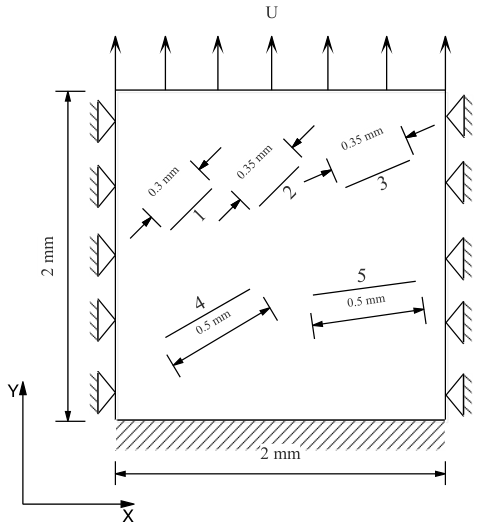
In this example, we first consider two cracks in a square plate of width $2$ mm, with the domain and boundary conditions shown in Fig. 19(a), to test the modeling of the junction between two cracks. Crack 1 is centered at ($-0.2,0$) with length $0.6$ mm and polar angle (relative to the horizontal direction) $9^{\circ}$, while Crack 2 is centered at ($0.46,0$) with length $0.8$ mm and polar angle $65^{\circ}$. The bottom edge of the domain is fixed and the top edge is fixed along $x$-direction while a uniform $y$-displacement $U$ is increased with time to drive the crack propagation. The material parameters are the same as previous examples, that is, elastic constants $\lambda=121.15$ kN/mm², $\mu=80.77$ kN/mm², and the fracture toughness is $g_{c}=2.7\times 10^{-3}$ kN/mm. The displacement increment is chosen as $\Delta U=1\times 10^{-4}$ mm for the computation. The mesh consists of $10,000$ triangular elements and the length scale parameter is chosen as $l=0.00375$ mm. A similar configuration with different boundary conditions has been used by Budyn et al. [15].

Typical adaptive meshes and contours of the phase-field variable during crack evolution are shown in Fig. 20. As can be seen, the mesh adapts dynamically to capture the junction process of the two cracks. As the load $U$ increases, the evolution can be described as follows.

• (a)

  $U=8\times 10^{-3}$ mm: the tip of Crack 1 activates;

• (b)

  $U=8\times 10^{-3}$ to $1.0\times 10^{-2}$ mm: Crack 1 propagates along a curved path heading towards Crack 2;

• (c)

  $U=1.1\times 10^{-2}$ mm: Crack 1 connects to Crack 2, and one of the tip for Crack 2 activates;

• (d)

  $U=1.6\times 10^{-2}$ mm: both Crack 1 and Crack 2 have propagated to the edge of the plate.

Since there is no analytical solution for this problem, we cannot compare the computed solutions with the exact solution. Nevertheless, they can be justified in physics. In fact, it is known (e.g., see [46]) that the critical stress increases as the polar angle increases and cracks with large polar angles are harder to initiate. Therefore, Crack 1, which is oriented with a smaller polar angle, is the first to initiate and propagate. Moreover, the frequency of crack coalescence is strongly related to the crack density (the crack size and their relative location) within the solid; e.g., see [55]. The higher the crack density is, the more likely two cracks will merge. Since being close to Crack 2, Crack 1 begins to merge with Crack 2 as it grows. At the same time, the other side of Crack 1 has propagated to the edge of the plate, which causes the left of the plate to lose strength. At later stages, the right side of the tip for Crack 2 activates and propagates to the edge of the plate.

Next, we consider five initial cracks in the same domain and with the same boundary conditions as for the two-crack problem, see Fig. 19(b). The material parameters are the same as previous examples except $g_{c}=2.7\times 10^{-4}$ kN/mm. The lengths of Crack 1, 2, 3, 4, and 5 are $0.3$ mm, $0.35$ mm, $0.35$ mm, $0.5$ mm, and $0.5$ mm, centered at ($-0.6,0.3$), ($0,0.5$), ($0.6,0.5$), ($-0.5,-0.4$), and ($0.5,-0.2$), with polar angle $30^{\circ}$, $45^{\circ}$, $17^{\circ}$, $28.6^{\circ}$, and $9^{\circ}$, respectively.

References

- [1] M. Ambati, T. Gerasimov, and L. D. Lorenzis. A review on phase-field models of brittle fracture and a new fast hybrid formulation. Comput. Mech., 55:383–405, 2015.
- [2] L. Ambrosio and V. M. Tortorelli. Approximation of functionals depending on jumps by elliptic functionals via -convergence. Comm. Pure Appl. Math., 43:999–1036, 1990.
- [3] H. Amor, J.-J. Marigo, and C. Maurini. Regularized formulation of the variational brittle fracture with unilateral contact: Numerical experiments. J. Mech. Phys. Solids, 57:1209–1229, 2009.
- [4] W. K. Anderson, J. L. Thomas, and B. V. Leer. Comparison of finite volume flux vector splittings for the Euler equations. AIAA Journal, 24:1453–1460, 1986.
- [5] M. Artina, M. Fornasier, S. Micheletti, and S. Perotto. Anisotropic mesh adaptation for crack detection in brittle materials. SIAM J. Sci. Comput., 37:B633–B659, 2015.
- [6] H. Azadi and A. R. Khoei. Numerical simulation of multiple crack growth in brittle materials with adaptive remeshing. Int. J. Numer. Meth. Eng., 85:1017–1048, 2010.
- [7] M. J. Baines. Moving Finite Elements. Oxford University Press, Oxford, 1994.
- [8] M. J. Baines, M. E. Hubbard, and P. K. Jimack. Velocity-based moving mesh methods for nonlinear partial differential equations. Commun. Comput. Phys., 10:509–576, 2011.
- [9] M. J. Borden. Isogeometric Analysis of Phase-field Models for Dynamic Brittle and Ductile Fracture. The University of Texas at Austin, 2012. PhD thesis.
- [10] M. J. Borden, C. V. Verhoosel, M. A. Scott, T. J. R. Hughes, and C. M. Landis. A phase-field description of dynamic brittle fracture. Comput. Methods Appl. Mech. Eng., 217:77–95, 2012.
- [11] M. J. Borden, T. J. R. Hughes, C. M. Landis, and C. V. Verhoosel. A higher-order phase-field model for brittle fracture: formulation and analysis within the isogeometric analysis framework. Comput. Methods Appl. Mech. Eng., 273:100–118, 2014.
- [12] P. O. Bouchard, F. Bay, Y. Chastel, and I. Tovena. Crack propagation modelling using an advanced remeshing technique. Comput. Methods Appl. Mech. Eng., 189:723–742, 2000.
- [13] B. Bourdin, G. A. Francfort, and J. J. Marigo. Numerical experiments in revisited brittle fracture. J. Mech. Phys. Solids, 48:797–826, 2000.
- [14] C. Budd, W. Huang, and R. Russell. Adaptivity with moving grids. Acta Numerica, 18:111–241, 2009.
- [15] E. Budyn, G. Zi, N. Moës, and T. Belytschkoi. A method for multiple crack growth in brittle materials without remeshing. Int. J. Numer. Mech. Engng., 61:1741–1770, 2004.
- [16] Q. Du and J. Zhang. Adaptive finite element method for a phase field bending elasticity model of vesicle membrane deformations. SIAM J. Sci. Comput., 30:1634–1657, 2008.
- [17] G. A. Francfort and J. J. Marigo. Revisiting brittle fracture as an energy minimization problem. J. Mech. Phys. Solids, 46:1319–1342, 1998.
- [18] P. E. Farrell and C. Maurini. Linear and nonlinear solvers for variational phase-field models of brittle fracture. Int. J. Numer. Meth. Engng., 109: 648–667, 2017.
- [19] T. Gerasimov and L. D. Lorenzis. A line search assisted monolithic approach for phase-field computing of brittle fracture. Comput. Methods Appl. Mech. Eng., 312:276–303, 2016.
- [20] T. Heister, M. F. Wheeler, and T. Wick. A primal-dual active set method and predictor-corrector mesh adaptivity for computing fracture propagation using a phase-field approach. Comput. Methods Appl. Mech. Eng., 290:466–495, 2015.
- [21] W. Huang. Variational mesh adaptation: isotropy and equidistribution. J. Comput. Phys., 174:903–924, 2001.
- [22] W. Huang. Practical aspects of formulation and solution of moving mesh partial differential equations. J. Comput. Phys., 171:753–775, 2001.
- [23] W. Huang. Mathematical principles of anisotropic mesh adaptation. Comm. Comput. Phys., 1:276–310, 2006.
- [24] W. Huang and L. Kamenski. A geometric discretization and a simple implementation for variational mesh generation and adaptation. J. Comput. Phys., 301:322–337, 2015.
- [25] W. Huang and L. Kamenski. On the mesh nonsingularity of the moving mesh pde method. Math. Comp., (to appear).
- [26] W. Huang, Y. Ren, and R. D. Russell. Moving mesh methods based on moving mesh partial differential equations. J. Comput. Phys., 113:279–290, 1994.
- [27] W. Huang, Y. Ren, and R. D. Russell. Moving mesh partial differential equations (mmpdes) based upon the equidistribution principle. SIAM J. Numer. Anal., 31:709–730, 1994.
- [28] W. Huang and R. D. Russell. Adaptive Moving Mesh Methods. Springer, New York, 2011. Applied Mathematical Sciences Series, Vol. 174.
- [29] W. Huang and W. Sun. Variational mesh adaptation II: error estimates and monitor functions. J. Comput. Phys., 184:619–648, 2003.
- [30] A. R. Khoei, H. Azadi, and H. Moslemi. Modeling of crack propagation via an automatic adaptive mesh refinement based on modified superconvergent patch recovery technique. Eng. Fract. Mech., 75:2921–2945, 2008.
- [31] R. Kobayashi. Modeling and numerical simulations of dendritic crystal growth. Physica D, 63:410–423, 1993.
- [32] C. Kuhn and R. Muller. A continuum phase field model for fracture. Eng. Frac. Mech., 77:3625–3634, 2010.
- [33] C. Kuhn, A. Schluter, and R. Muller. On degradation functions in phase field fracture models. Comput. Materials Sci., 108:374–384, 2015.
- [34] C. Liu and J. Shen. A phase field model for the mixture of two incompressible fluids and its approximation by a Fourier-spectral method. Phys. D, 179:211–228, 2003.
- [35] G. Liu, Q. Li, and Z. Zuo. Implementation of a staggered algorithm for a phase field model in ABAQUS. C. J. Rock Mech. Eng., 35:1019–1030, 2016.
- [36] J. A. Mackenzie and M. L. Robertson. A moving mesh method for the solution of the one-dimensional phase-field equations. J. Comput. Phys., 181:526–544, 2002.
- [37] J. R. Magnus. On differentiating eigenvalues and eigenvectors. Econometric Theory, 1:179–191, 1985.
- [38] S. May, J. Vignollet, and R. de Borst. A numerical assessment of phase-field models for brittle and cohesive fracture: -convergence and stress oscillations. European J. Mech. A/Solids, 52:72–84, 2015.
- [39] C. Miehe. Comparison of two algorithms for the computation of fourth-order isotropic tensor function. Comput. Struct., 66:37–43, 1998.
- [40] C. Miehe, M. Hofacker, and F. Welschinger. A phase field model for rate-independent crack propagation: Robust algorithmic implementation based on operator splits. Comput. Methods Appl. Mech. Eng, 199:2765–2778, 2010.
- [41] C. Miehe and M. Lambrecht. Algorithms for computation of stresses and elasticity moduli in terms of Seth-Hill’s family of generalized strain tensors. Commun. Numer. Meth. Engng., 17:337–353, 2001.
- [42] C. Miehe, F. Welschinger, and M. Hofacker. Thermodynamically consistent phase-field models of fracture: Variational principles and multi-field FE implementations. Int. J. Numer. Meth. Eng, 83:1273–1311, 2010.
- [43] N. Moës and J. Dolbow and T. Belytschko. A finite element method for crack growth without remeshing. Int. J. Numer. Methods Eng., 46:131–150, 1999.
- [44] N. Moës and T. Belytschko. Extended finite element method for cohesive crack growth. Eng. Fract. Mech., 69:813–833, 2002.
- [45] T. T. Nguyen, J. Yvonnet, Q. Z. Zhu, M. Bornert, and C. Chateau. A phase field method to simulate crack nucleation and propagation in strongly heterogeneous materials from direct imaging of their microstructure. Eng. Frac. Mech, 139:18–39, 2015.
- [46] N. Perez. Fracture Mechanics. Kluwer Academic Publishers, New York, 2004.
- [47] S. Phongthanapanich and P. Dechaumphai. Adaptive Delaunay triangulation with object-oriented programming for crack propagation analysis. Fin. Elem. Anal. Design, 40:1753–1771, 2004.
- [48] J. Pokluda and P. Šandera. Micromechanisms of Fracture and Fatigue: In a Multi-scale Context. Springer-Verlag, London, 2010.
- [49] J. Shen and X. Yang. An efficient moving mesh spectral method for the phase-field model of two-phase flows. J. Comput. Phys., 228:2978–2992, 2009.
- [50] J. Shen and X. Yang. Decoupled energy stable schemes for phase-field models of two-phase complex fluids. SIAM J. Sci. Comput., 36:B122–B145, 2014.
- [51] J. Shen, X. Yang, and H. Yu. Efficient energy stable numerical schemes for a phase field moving contact line model. J. Comput. Phys., 284:617–630, 2015.
- [52] T. Tang. Moving mesh methods for computational fluid dynamics flow and transport. In Recent Advances in Adaptive Computation (Hangzhou, 2004), volume 383 of AMS Contemporary Mathematics, pages 141–173. Amer. Math. Soc., Providence, RI, 2005.
- [53] J. Vignollet, S. May, R. de Borst, and C. V. Verhoosel. Phase-field models for brittle and cohesive fracture. Meccanica, 49:2587–2601, 2014.
- [54] H. Wang, R. Li, and T. Tang. Efficient computation of dendritic growth with -adaptive finite element methods. J. Comput. Phys., 227:5984–6000, 2008.
- [55] Y. Z. Wang, J. D. Atkinson, R. Akid, and R. N. Parkins. Crack interaction, coalescence and mixed mode fracture mechanics. Fatigue Fract. Engng. Mater. Struct., 19:427–439, 1996.
- [56] A. A. Wheeler, B. T. Murray, and R. J. Schaefer. Computation of dendrites using a phase field model. Physica D, 66:243–262, 1993.
- [57] T. Wick. An error-oriented Newton/inexact augmented Lagrangian approach for fully monolithic phase-field fracture propagation. SIAM J. Sci. Comput., 39:B589–B617, 2017.
- [58] T. Wick. Modified Newton methods for solving fully monolithic phase-field quasi-static brittle fracture propagation. Comput. Methods Appl. Mech. Eng, 325:577–611, 2017.
- [59] X. Yang, J. J. Feng, C. Liu, and J. Shen. Numerical simulations of jet pinching-off and drop formation using an energetic variational phase-field method. J. Comput. Phys., 218:417–428, 2006.
- [60] X. Yang, J. J. Feng, C. Liu, and J. Shen. Numerical simulations of jet pinching-off and drop formation using an energetic variational phase-field method. J. Comput. Phys., 218:417–428, 2006.
- [61] P. Yu, L. Q. Chen, and Q. Du. Applications of moving mesh methods to the fourier spectral approximations of phase-field equations. In Recent Advances in Computational Sciences, pages 80–99, 2008. World Sci. Publ., Hackensack, NJ.