The expansion of tensor models with two symmetric tensors
Abstract
It is well known that tensor models for a tensor with no symmetry admit a expansion dominated by melonic graphs. This result relies crucially on identifying jackets which are globally defined ribbon graphs embedded in the tensor graph. In contrast, no result of this kind has so far been established for symmetric tensors because global jackets do not exist.
In this paper we introduce a new approach to the expansion in tensor models adapted to symmetric tensors. In particular we do not use any global structure like the jackets. We prove that, for any rank , a tensor model with two symmetric tensors and interactions the complete graph admits a expansion dominated by melonic graphs.
1 Introduction and discussion
The two main families of tensor models for a non symmetric tensor11 1 See [1, 2] for the algebraic properties of non symmetric tensors., the colored models [3, 4, 5, 6, 7] and the general invariant models [8, 9, 10] have been thoroughly studied over the past several years. Their expansion has been established in arbitrary rank [8, 4, 5, 6, 9, 11, 10] and, for some models, non perturbatively [12]. Similar results hold for the multi-orientable tensor model in rank [13, 14] In all cases, the large limit is dominated by melonic graphs [15]. The expansion in tensor models gives the third (and last) universality class of such expansions, different from both the vector and the matrix case. Starting from these results a new large limit in models with a large number of matrices [16, 17, 18] has been discovered.
However, the first tensor models considered in the literature [19, 20] were formulated for symmetric tensors. In spite of the many successes of the theory of random non symmetric tensors, until recently, there has been no result concerning the expansion in the symmetric case. Developments in a very different area bring a renewed interest in tensor models with symmetric tensors.
The Sachdev–Ye–Kitaev (SYK) model [21, 22], which is a model of fermions with quenched random couplings, provides in the large limit a one dimensional nearly conformal field theory which is the dual of a black hole in . This concrete realization of the duality has been studied in depth [23, 24, 25, 26, 27, 28]. The main feature of the SYK model is that its large limit is solvable. It turns out that this limit is solvable because the SYK model is a tensor model in disguise: the random tensor is the tensor of random couplings. As for all tensor models for which a large limit has been proven to exit, the large limit of the SYK model is dominated by melonic graphs[23, 24, 29]. The melonic large limit is universal [30] in non symmetric random tensors hence it is only natural to consider a tensor version of the SYK model [31, 32, 33, 34, 35, 36]. Besides eliminating the quenching, the tensor SYK models are genuine gauge theories and come equipped with a full set of invariant observables, clarifying in particular the status of the singlets in the usual SYK model. The corrections are also accessible in the tensor SYK models [37, 38]22 2 We note however that the results of [38] in this direction are only partial as they ignore the effect of the explicit breaking of conformality in the leading order four point function [23]. .
A feature of tensor models for non symmetric tensors is that they have a rather large gauge group consisting in many copies of the unitary or the orthogonal group [8]. In order to have a gauge theory for only one copy of the unitary or the orthogonal group, one would like to use symmetric or antisymmetric tensors.
The problem is that no result concerning the expansion for models with symmetric or antisymmetric tensors has so far been established. In fact, if a large limit exists for models with one symmetric tensor, it can not be dominated by melonic graphs: symmetric tensors generate a family of pathological graphs which scale faster with than the melonic family.
An elegant solution to this problem has been proposed recently by I. Klebanov and G. Tarnopolsky: in [39] the authors considered a model for a symmetric traceless tensor. The “tracelessness” condition eliminates the pathological graphs at low orders (up to order [39]). This led the authors to conjecture that tensor models for symmetric traceless (and antisymmetric) tensors in rank 3 have a expansion dominated by melonic graphs.
Proving this conjecture is impossible with the methods developed for the study of non symmetric tensors. Indeed, for non symmetric tensors one relies entirely on identifying jackets which are global ribbon graph embedded in the tensor graphs. Jackets do not exist for symmetric or antisymmetric tensors.
In this paper we introduce a new approach to the expansion adapted to symmetric (and antisymmetric) tensors. Crucially, we do not introduce any global structure like the jackets, but only local moves on the graphs which can be controlled.
We study here a model with two symmetric tensors in arbitrary rank. This is done for convenience. Indeed, while the same method is expected to work for one antisymmetric or symmetric traceless tensor, it is significantly more complicated to check. Using two tensors has several consequences:
- •
the graphs of the model are bipartite which drastically simplifies the analysis,
- •
in the symmetric case, the tensors need not be traceless and the propagator has only terms (in rank ) and not (see [39]).
Using this method to establish the expansion for models with one antisymmetric or one symmetric traceless tensor is straightforward. However, as establishing the expansion in the bipartite case is already somewhat involved, this generalization is expected to be quite challenging.
2 The model and its Feynman graphs
From now on denotes an integer larger or equal to . We consider two real symmetric tensors of rank , denoted and , transforming in the fundamental representation of the orthogonal group :
for any and permutation of elements. The action of the two tensor model with interaction in rank is:
| (1) | ||||
| (2) |
while in arbitrary rank it is33 3 In all rigor one defined the model as the limit of a model with covariance . We will spare the reader such tedious details.:
| (3) | ||||
| (4) |
where denotes addition modulo . Observe that if one represents each tensor as a vertex and each contraction of two indices as an edge, the contraction pattern of the indices in the interaction term reproduces the complete graph with vertices, . The action has an gauge invariance, for any . We stress that the gauge group is just one copy of the orthogonal group. Our aim is to evaluate the two point function of the model:
The two point function is a sum over connected, stranded Feynman graphs, where each strand represents an index of the tensor [3, 4, 6]. One edge of the graph is marked with an oriented arrow and represents the insertion (and the arrow is oriented from to ). The vertex and the propagator of the model in and are depicted in Fig.1.

Due to the symmetry of the tensors there are distinct contributions to the propagator:
where the subscript zero indicates that the expectation is taken at . In for instance the propagator is the sum of six terms:
The strands of the propagator always connect an index at one end of the propagator to an index at the other end. This is different from the traceless model of [39], where indices on the same side of the propagator can be connected by a strand (the extra terms one can find in the propagator of [39]). Adding such terms is quite tedious, and this is one of the challenges of dealing with models with only one tensor. However, we stress that these extra terms are crucial in the one tensor case, as they actively kill the pathological contributions in the Feynman expansion. Luckily, the two tensor model we deal with here does not generate the pathological contributions to begin with and one can just use symmetric tensors with no tracelessness condition.
The Feynman graphs are built by gluing stranded propagators on the stranded vertices: strands are glued together and ultimately close into the faces of the graph. Observe that, as the propagator only connects a and a , the Feynman graphs are bipartite. This will prove crucial later on.
When computing the Feynman amplitude of a connected graph one obtains a free sum over an index for every face of the graph and an explicit scaling factor for every vertex. Denoting the number of vertices of a connected graph , the number of its faces, and taking into account the explicit prefactor the amplitude of is:
where we define the degree of a connected graph to be:
| (5) |
and the degree of a disconnected graph to be the sum of the degrees of its connected components.
In principle the degree of a graph can be any integer44 4 The number of vertices of any graph is even as the graphs are bipartite: positive, zero or negative. A tensor model has a expansion if, for all the graphs, the degree is non negative and there exist graphs of degree . This ensures that the two point function of the model has a non trivial large limit. If the two point function has a non trivial large limit, then the free energy per degree of freedom and the expectations of invariant observables will also have non trivial large limits.
Non symmetric tensors.
Let us briefly recall how the expansion works for non symmetric tensors [3, 4, 6, 8, 9] The Feynman graphs can still be represented as stranded graphs (although more concise representations as colored graphs exist), but in the stranded representation all the propagators have parallel strands. Using this, one can define global jackets which are ribbon graphs embedded in a tensor graph and use them to count the number of faces. It turns out that the degree is the average genus of the jackets, hence, in particular, non negative. It follows that the tensor models for non symmetric tensors admit a expansion. This works for the colored models [4, 6], the invariant models [8, 10] and the multi orientable model [13, 14].
The leading order graphs (of degree ) are called [15] melonic and have a very simple structure. Several equivalent definitions of melonic graphs exist [15, 11]. Observe that the zero order contribution to the two point function is represented as a graph with no vertex, consisting in one (marked) edge closing onto itself. We call this graph the ring graph. It is the melonic graph of degree .
Definition 1.
(See Fig. 2) A graph is called melonic if:
- •
either is the ring graph,
- •
or can be obtained from a melonic graph with strictly fewer vertices by inserting two vertices connected by edges on one of the edges of .

For tensor models of rank , the vertices should be interpreted as stranded vertices and the edges as stranded edges with parallel strands. It is easy to check that all the melonic graphs have degree zero. It is slightly less trivial to show [15] that for non symmetric tensors a graph of degree zero must be melonic.
The key to the expansion for non symmetric tensors is the existence of the jackets. For example in the simplest jacket [40] (there are another two jackets for [4]) is obtained by deleting the middle stands on all the propagators. As the propagators all have parallel strands, a middle strand will always connect to a middle strands, and deleting the middle strands leaves just the outer strands on all the vertices which form a well defined ribbon graph.
Symmetric tensors.
All this fails if the tensors have some symmetry properties. Indeed, for symmetric or antisymmetric tensors one must allow an arbitrary permutation of the strands along the propagators. In this case there is no notion of “middle” and “outer” strands, and no way to obtain a ribbon graph embedded in the tensor graph. For instance, in the case presented in Fig. 3, if one attempts to delete the blue face, one obtains a residual graph which has one propagator with three strands, and another three propagators with only one strand.
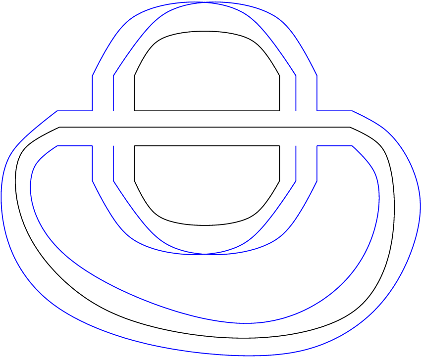
For this reason, if one wants to establish the expansions in models involving symmetric or antisymmetric tensors, one needs to find a completely new approach to the problem. This is what we do in this paper.
3 The expansion for two symmetric tensors
Embeddings.
Using the symmetries of the tensors one can always embed the graphs in the plane in a convenient manner. Any edge connects a vertex and a vertex . By permuting the half edges around one of the vertices, an edge can always be embedded such that all the strands of the edge are parallel. There are such embeddings corresponding to a simultaneous permutation of all the half edges on and all the half edges on .
In fact, for any combinatorial tree in a graph, one can always chose an embedding such that all the edges in the tree are embedded with parallel strands. This is done by untwisting the edges starting from some arbitrary root vertex. This fixes iteratively the order of the half edges around every vertex in the graph. We stress that the choice of the combinatorial tree fixes the embedding as a plane tree, that is the remaining half edges of the graph have assigned positions around the vertices of the tree. The loop edges, which pair the remaining half edges together, are then embedded with nontrivial permutations of strands and can cross55 5 One can eliminate the crossing by embedding in a higher genus surface but the permutations of the strands can not be eliminated..
Rings.
As arbitrary permutations of the strands are allowed one obtains ring graphs. They have no vertices (indeed they are the only “bipartite” stranded graphs with zero vertices) and at most faces, hence, from Eq. (5), have non negative degree. We depicted in Fig. 4 the ring graphs in . They have degrees, from left to right , and .
The ring graph with identity permutation on the strands is the only one which has exactly faces and degree . We call it the melonic ring graph.

Graphs with two vertices.
As the graphs are bipartite, a graph with two vertices has edges which connect the two vertices (in particular the graph is always connected).
Lemma 1.
A graph with two vertices has non negative degree.
Proof.
A vertex contributes corners to the faces. If a graph has two vertices, it has a total of corners and, as a face has at least two corners, we have:
∎

Remark 1.
Graphs with two vertices and degree 0. Let us consider a graph with two vertices and degree zero. This graph can always be embedded in the plane in such a way that all the edges have parallel strands as in Fig. 5. In order to show this, let us introduce some notation.
We label the two vertices of the graph and and we label the marked edge (with the arrow pointing from to ). We can always embed the graph is the plane is such a way that all the strands of the edge are parallel. This fixes the order of the remaining half edges around both vertices66 6 Up to an irrelevant simultaneous permutation of the half edges on and .. Starting from the edge , we label the half edges turning counterclockwise around the vertex and respectively turning clockwise around the vertex . Every strand going through the vertex belongs to two half edges of and forms a corner. We label a strand (and the corresponding corner) by the couple of labels of the half edges: for instance denotes the strand common to the half edges and on and so on.
Now, every face has two corners. For any , the corner and are connected along the edge , and they must be connected by a second edge, hence necessarily the half edges and are connected by an edge. We label this edge . Finally, for every , the corner belongs to a face which goes trough the edges and . As every face has length two, this face must close trough one corner of the vertex , but the only corner common to the halfedge and is . Using this iteratively proves that all the edges are embedded with parallel strands.
Because arbitrary permutations of the strands are allowed, we must adapt the definition of melonic graphs to our case.
Definition 2.
A graph is called melonic if it admits an embedding such that:
- •
either is the melonic ring graph,
- •
or can be obtained from a melonic graph with strictly fewer vertices by inserting two vertices connected by parallel (embedded) edges with parallel strands on one of the edges of .
We have so far proven that the graphs with zero or two vertices have non negative degree and they have zero degree if only if they are melonic in the sense of Definition 2,
Graphs with more than two vertices.
We turn our attention to general graphs. Let us denote the number of faces with corners (i.e. of length ) of a graph . Observe that, as is bipartite, the faces can only have even length. The faces of length play a distinguished role.
Lemma 2.
If a nontrivial connected graph has no face of length two, then it has strictly positive degree.
Proof.
A vertex contributes corners to the faces, hence:
and if we have:
∎
A more refined statement can be made.
Proposition 1.
Consider a connected graph with more than two vertices and assume that for every vertex in , at most corners belong to faces of length two and the remaining corners belong to faces of length at least four. Then has strictly positive degree.
Proof.
We can rewrite the relation between the length of the faces of and the number of vertices of as:
The total number of faces of a graph is then bounded by:
and consequently the degree is bounded by:
Now, let us assume that at most corners of any vertex belong to faces of length two. Then , and:
∎
If the conditions in the hypothesis of Proposition 1 are not met, we have the following result.
Proposition 2.
If a connected graph with more than two vertices has a vertex such that at least corners of the vertex belong to faces of length two, then there exists a (possibly disconnected) graph having strictly fewer vertices such that the degree of is not larger than the one of , .
Proof.
See Section. 4 ∎
We emphasize that can be disconnected and some of its connected components can be ring graphs. The expansion of the model defined by Eq. 1 and Eq. (3) is encoded in the following theorem.
Theorem 1.
For any connected graph , .
Proof.
If has no vertex such that at least corners of the vertex belong to faces of length two, we conclude by Proposition 1. If has such a vertex, from Proposition 2 its degree is greater or equal than the one of a (possibly disconnected) graph having fewer vertices. We iterate on the connected components of . The end graphs of the iteration either have no vertex such that at least of its corners belong to faces of length two, hence have strictly positive degree from Proposition 1, or they have exactly two vertices, hence have non negative degree by Lemma 1. ∎
The rest of this paper is quite technical.
4 Proof of Proposition 2
4.1 Dipoles
Any face of length two is bounded by two edges connecting a pair of vertices. The converse however is not true: not any pair of edges connecting two vertices bounds a face of length two.
Definition 3.
For , we call a –dipole two vertices ( and ) connected by exactly edges. We call the parallel edges internal and the other edges hooked to the vertices of the dipole external.
A –dipole has:
- •
strands of length one coming from the internal edges.
- •
internal corners formed by the internal edges: on the vertex and on the vertex .
- •
mixed corners formed by an internal and an external edge: with the external edges incident at the vertex and with the external edges incident at the vertex .
- •
external corners formed by couples of external edges: between the external edges incident at and between the external edges incident at .
- •
internal faces which only pass through internal corners.
- •
vertical external faces passing through only one external corner each, which connect external edges on the same side of the dipole (either both on or both on ).
- •
horizontal external faces involving either only mixed corners or mixed and internal corners. The horizontal faces can connect either two external edges on different sides of the dipole or two external edges on same side of the dipole. A horizontal external face which connects a and a (or a and a ) has even length, and it has odd length if it connects a and a .
As the internal faces have at least length two, . If we say that the dipole is saturated (and in this case all the internal faces have length exactly two), and we say it has deficit if not.
4.2 –dipoles
We first assume that the graph (which by the hypothesis of Proposition 2 has a vertex such that at least corners of the vertex belong to faces of length two) has a –dipole. We then conclude by the following Proposition.
Proposition 3.
If a graph connected graph has a –dipole (saturated or not), then there exists a connected graph having strictly fewer vertices such that the degree of is not larger than the degree of , .
Proof.
Let us label the external half edges of the -dipole by and , and the internal edges . The dipole has internal faces, horizontal external faces and no vertical external face. Among the horizontal external faces traverse the dipole from to , and do not, hence they return and close on the same external half edge (see Fig. 6, bottom left).
A –dipole can be deleted by deleting the two vertices and and all the internal faces of the dipole, and reconnecting the external half edges by strands which traverse. For this reconnection we keep in place all the traversing strands, and pick any pairing of left and right returning strands, which we break and reconnect by two traversing strands (see Fig. 6, bottom right). At the end of this procedure we obtain a graph having and because every reconnection of returning external strands deletes at most a face of . Every propagator brings strands of length , therefore we have a total of strands. They divide into internal faces (each of which has length at least ) and external strands. The external strands have either odd length, in which case they are traversing, or even length, in which case they are returning. We obtain:
It follows that:
therefore, as , the degree can not increase with the deletion.

∎
4.3 Graphs with no –dipoles
We now assume that the graph does not have any –dipole. Then any two vertices in can be connected by at most edges.
By the hypothesis of Proposition 2, has a vertex such that at least corners of the vertex belong to faces of length two. As a function of the dimension we have several cases:
- For .
-
In order for a vertex in to be incident to at least a face of length , the vertex must belong to a saturated –dipole.
- For .
-
In order for a vertex in to be incident to at least faces of length , the vertex must:
- •
belong to a saturated –dipole,
- •
or belong to a –dipole with deficit and to another saturated –dipole.
Indeed, if a vertex belongs to a –dipole with deficit at least , then even adding a saturated –dipole can not add enough faces of length two on the vertex. If the graph has no –dipoles then a vertex can belong to at most two saturated –dipoles, hence be incident to at most two faces of length two.
- •
- For .
-
In order for a vertex in to be incident to at least faces of length , the vertex must:
- •
belong to saturated –dipole,
- •
or belong to a –dipole with deficit and to another saturated –dipole,
- •
or belong to two saturated –dipoles.
Indeed, if a vertex belongs to a –dipole with deficit at least , then even adding a saturated –dipole can not add enough faces of length two on the vertex. If a vertex does not belong to a –dipole, then it can belong to two different –dipoles, but if at least one of them is not saturated, then the vertex is incident to at most faces of degree two. In all other cases, at most faces of length two can meet at the vertex.
- •
- For .
-
In order for a vertex in to be incident to at least faces of length , the vertex must:
- •
belong to a saturated –dipole,
- •
or belong to a –dipole with deficit and to another saturated –dipole.
Indeed, if a vertex belongs to a –dipole with a larger deficit, then even adding a saturated –dipole can not add enough faces of length two on the vertex. If a vertex does not belong to a –dipole, then the largest number of faces of length two incident at the vertex is attained if the vertex belongs to a saturated –dipole and a saturated –dipole, and this number is:
- •
The situation is presented in Fig. 7.

4.3.1 Saturated –dipole
If has a saturated –dipole we conclude by the following Proposition.
Proposition 4.
If a connected graph has a saturated –dipole, then there exists a (possibly disconnected) graph having strictly fewer vertices such that the degree of is not larger than the degree of , .
Proof.
Let us label the external half edges of the –dipole by , and . As the dipole is saturated, all the internal corners are paired into internal faces of length . The dipole has two vertical external faces going through one external corner each. The horizontal external faces can not go through any internal corner (as none is available), hence always connect two mixed corners. This can also be seen as follows: the edges bring a total of strands of length , out of which belong to the internal faces. As mixed corners must be paired and there are exactly remaining strands, it follows that all the horizontal external faces of the dipole have length , and they connect one of the half edges or with one of the half edges and in one step.
After at most a relabeling (if needed) of the the half edges and , two of the horizontal external faces of the dipole will be and . In Fig. 8 we presented a saturated –dipole and, at the bottom left, its external faces.

The vertical external faces connect with and with . Any edge of the dipole has exactly strands involved in the internal faces and strands forming two horizontal external faces. The horizontal external faces always go from left () to right (). If is connected to (respectively ) by a strand of the edge then, as has strands but of them are involved in the internal faces, must connect to (respectively .
If we are in the case and we say that the couple of faces is parallel (as they are parallel with the two horizontal external faces and ) and we denote the number of such couples of external faces (including the couple of faces and ). If not, we say that the couple of faces is crossing, and we denote the number of couples of faces which are crossing by . We have:
A saturated –dipole can be deleted by deleting the two vertices and and all the internal faces of the dipole and reconnecting the external half edges to form two new edges. This can be done in two ways:
- The parallel channel.
-
In the parallel channel one joins the half edge with the half edge and the half edge with the half edge . The parallel horizontal external faces are left untouched, but the crossing horizontal external faces (and the two vertical external faces) are opened and reconnected as depicted in Fig. 8. One performs reconnections in this case.
- The crossing channel.
-
In the crossing channel one joins the half edge with the half edge and the half edge with the half edge . The crossing horizontal external faces are left untouched, but the parallel horizontal external faces (and the two vertical external faces) are opened and reconnected as depicted in Fig. 8. One performs reconnections in this case.
Each reconnection can at most decrease the number of faces by (if the two faces of involved in the reconnection are different). However, if the two strands which are broken and reconnected belong to the same face of , the reconnection can create a face and increase the number of faces by or it can leave it unchanged. The graph can have two connected components in which case we say that the deletion is separating. We have several cases:
- The case .
-
If , we perform a deletion in the parallel channel. Two sub cases arise:
- •
Separating deletion. If the deletion is separating, then splits into two connected components: containing the new edge and containing the new edge . In this case, following the vertical external face of the dipole in as it enters the (future) connected component , we notice that it can exit only through the second vertical external face of the dipole , hence the breaking and regluing of the vertical external strands will split a face of into two different faces in and , thus:
- •
Non separating deletion If the deletion is non separating, then and:
- •
- The case .
-
If , we can perform a deletion in either of the two channels. Observe that the deletion can not be separating in both channels at the same time. Choosing a channel which is not separating we have:
∎
4.3.2 –dipole with deficit and saturated –dipole
If has a vertex belonging to a –dipole with deficit and to a saturated –dipole we conclude by the following Proposition.
Proposition 5.
For , if a connected graph has a vertex belonging to a –dipole with deficit and to a saturated –dipole, then there exists a connected graph having strictly fewer vertices such that the degree of is strictly smaller than the degree of , .
Proof.
We use the same notation as in Proposition 4 and assume that the vertex belonging to a saturated –dipole is : the only way for to have corners belonging to faces of length two is for the corner to belong to such a face.
Let us detail the structure of the –dipole. As it has exactly faces of length two, several cases are possible:
- Short horizontal faces.
-
internal corners on each vertex are paired in faces of length two, and the remaining internal corners ( on each vertex) all belong to the same internal face of length . The analysis of Proposition 4 goes through: the horizontal external faces can not go through any internal corner (as none is available), hence always connect two mixed corners directly. Every edge has two mixed corners at each end of the edge and respectively and , which are connected either parallel or crossing. The external faces of the dipole have the same structure as in the case of the saturated –dipole, reproduced in Fig. 9.

Figure 9: External faces of a –dipole with deficit and short horizontal external faces. - Long horizontal faces.
-
Another possibility is to have internal corners on each vertex paired in faces of length . The two remaining internal corners are and for some . As , one can always chose and embed the edge with parallel strands as before. The edges and only have strands belonging to internal faces, and strands belonging to the external faces. The edges have, as before, strands belonging to internal faces and strands belonging to external faces. The external faces passing through the edges have as before length (and can be either parallel or crossing).
There are several cases:
- •
both and belong to the same horizontal face of length three. In this case again the structure of the external faces is identical to the one of the saturated –dipole reproduced in Fig. 9.
- •
each one of the two corners and belongs belongs to a different horizontal face of length two. Then one horizontal face originating on the vertex must go back to the vertex (passing through the corner ), and one face originating on the vertex must go back to the vertex (passing through the corner ). The other external faces are as before and have length . All the possibilities of connections of external faces are presented in Fig. 10.

Figure 10: External faces for –dipoles with deficit . We represented in red (respectively blue) the external faces with length (respectively ) involving the edges and .
- •
As long as the external faces have the same structure as in the case of the saturated –dipole, we perform the deletions as in Proposition4. The only difference is that one less internal face is deleted, hence in all cases the degree strictly decreases:
It remains to perform the deletions in the cases presented in Fig. 10. Observe that we can start by breaking the two red external faces and reconnect them the other way around, such that each of them goes from to making sure that the new red faces can be paired with the blue faces into either parallel or crossing pairs (each pair has a red and a blue face). This can decrease the number of faces in by , but the –dipole has deficit . Observe that the deletion can not be separating in any channel (as both edges and connect on the same vertex, the second vertex of the saturated –dipole). It follows that, in the notation of Proposition4:
for all . ∎
4.3.3 Two saturated –dipoles in
This concerns only the case . If has a vertex belonging to two saturated –dipoles, we conclude by the following Proposition.
Proposition 6.
For , if a connected graph has a vertex belonging to two saturated –dipoles, then there exists a connected graph having strictly fewer vertices such that the degree of is strictly smaller than the degree of , .
Proof.
Let us consider a saturated –dipole in . We label its internal edges and , and the external half edges and on both vertices. We delete the dipole and reconstruct three edges. There are six possible channels of deletion: the half edge can be connected with any half edge or and so on.

In the process the three internal faces of length two are deleted, and three vertical external faces must be broken and reconnected (in the channel , , for instance the external faces and are cut and reglued into two faces and , and are cut and reglued into and respectively and finally are cut and reglued into and ). We will show below that in all cases at most three cuts and regluings of horizontal external faces are needed in order to create the remaining faces of the new edges. As the number of faces goes down by at most one for each cut and reglue, we have in all cases and:
The external faces of the dipole have the structure presented in Fig. 12.

We embed the dipole it in the plane with the edge with parallel strands (which can always be done after at most a relabeling of the half edges and ). The external faces going through the edges (in blue in Fig. 12) and (in red Fig. 12) are connected by arbitrary permutations. We denote the permutation on the edge (respectively ) by (respectively ), that is the corner is connected by a strand to and so on. Both and are permutations over three elements and are (in cycle notation) either even or odd , and .
We always delete the dipole in the channel , and . If the permutation is odd, it can be turned into the identity permutation by one cut and regluing of faces. If is even, two cuts are needed. We have the following cases:
- •
One of or is the identity. Then at most two cuts are needed.
- •
At least one of or is odd. Then at most three cuts are needed.
- •
and is even. By permuting the half edges on the right to both the edges and are embedded with parallel strands (but the edge picks up the permutation ). Reconnecting the edges in the channel , and , at most two cuts are needed.
- •
Both and are even, neither of the two is the identity and they are different. Then three cuts are needed. Let’s assume that and . We then:
- –
cut the blue (defined by ) face and the red (defined by ) face and reglue then as two faces and ,
- –
cut the blue (defined by ) face and the red (defined by ) face and reglue then as two faces and ,
- –
cut the blue (defined by ) face and the red (defined by ) face and reglue then as two faces and .
Observe that the new faces mix a blue and a red, that is we cut and reglue faces which used to go through different internal propagators in the dipole.
- –
∎
5 The leading order
In this last section we identify the leading order graphs of degree zero. Their classification relies on Theorem 1. We have the following result.
Lemma 3.
If a connected graph has degree , then the strands of any edge in belong to different faces of .
Proof.
Take any edge in and cut it. As is bipartite, the cut can not disconnect and one obtains a two point graph . If faces of are cut, then the number of internal faces of is:
We build a graph by connecting a chain of graphs together. We have:
therefore:
which becomes arbitrarily negative for large enough, contradicting Theorem 1. ∎
Corollary 1.
If a connected graph of degree 0 has a –dipole, then the –dipole is saturated.
Proof.
As has degree zero, a –dipole in can not have any horizontal external faces which return on the same external edge. In the notation used in Proposition3, we have and . The degree of the graph can not decrease with the deletion of the –dipole, hence the dipole must have exactly internal faces. ∎
From Proposition 1 and Section 4 we conclude that a graph with degree zero can only have:
- •
a –dipole, which in view of Corollary 1 is saturated. The –dipoles can be deleted iteratively.
- •
or has a saturated –dipole such that:
- –
the –dipole has and the deletion in the parallel channel is separating,
- –
or the –dipole has but then one of the three must hold:
- *
and the deletion is separating in the parallel channel,
- *
and the deletion is separating in the crossing channel,
- *
, and the deletion is not separating in either channel.
- *
- –
In the last case, in Proposition 4 we chose to perform the deletion in the non separating channel, and the degree did not increase with the deletion. For graphs of degree zero, we proceed differently. We show that in fact the last three cases are excluded.
Proposition 7.
If a connected graph has a saturated –dipole which is either:
- •
and separating in the parallel channel,
- •
and separating in the crossing channel,
then .
Proof.
Assume that a graph with degree zero has such dipoles. The two cases are represented in Fig. 13

By performing the –dipole deletion in the separating channel, splits into two graphs and , such that the new edge belongs to and the new edge belongs to . By Theorem 1, both and have non negative degree:
Observe that we have not proven that the deletion of such –dipoles in the separating channel does not increase the degree. In Proposition 4 we have only shown that the deletion in the non separating channel does not increase the degree, but nothing is know so far about the deletion in the separating channel: in principle and could have strictly positive degrees.
Following in the strands as they enter one of the connected components and taking into account that, by Lemma 3, on any edge in the strands must belong to different faces, it follows that the external faces of the dipole necessarily have the structure in Fig. 13. We have in both cases:
hence:
which contradicts the assumption that had zero degree. ∎
Finally, the last case is excluded by the following Proposition.
Proposition 8.
In , if a connected graph has a non separating –dipole with then .
Proof.
Assume that a graph of degree zero has such a dipole. Observe the faces and , the faces , and and the faces and must all be different, otherwise there exists a deletion channel of the –dipole in which the number of faces goes down by only (instead of going down by ) and the degree strictly decreases by performing the deletion in this channel. Taking this and Lemma 3 into account, the structure of the external faces of the dipole must be the one presented in in Fig. 14.

By cutting the four edges incident to the dipole one obtains a four point graph , having internal faces and:
hence . One can chain several copies of and build a graph as depicted in Fig. 15.

The number of faces and vertices of a chain of length is:
hence the degree of the chain graph is:
which can be arbitrarily negative, contradicting Theorem1. ∎
Theorem 2.
A graph has degree zero if and only if it is melonic in the sense of Definition 2.
Proof.
From the previous discussion we conclude that a graph of degree zero reduces to a union of melonic graphs with two vertices by iterated deletions of:
- •
saturated –dipoles,
- •
completely separating deletions of saturated –dipoles with .
Observe that both the saturated –dipoles and the saturated –dipoles with can be embedded in the plane in such a way that that all the edges are embedded as parallel edges with parallel strands. Obviously all graphs of degree are generated by doing the reverse, namely adding saturated –dipoles or joining at separating, saturated , –dipoles. ∎
References
- [1] I. Gelfand, M. Kapranov, and A. Zelevinsky, Discriminants, resultants and multidimensional determinants. Birkhauser, Boston, 1994.
- [2] P. Diaz and S.-J. Rey, “Orthogonal Bases of Invariants in Tensor Models,” 1706.02667.
- [3] R. Gurau, “Colored Group Field Theory,” Commun. Math. Phys. 304 (2011) 69–93, 0907.2582.
- [4] R. Gurau, “The expansion of colored tensor models,” Ann. H. Poincaré 12 (2011) 829–847, 1011.2726.
- [5] R. Gurau and V. Rivasseau, “The expansion of colored tensor models in arbitrary dimension,” Europhys. Lett. 95 (2011) 50004, 1101.4182.
- [6] R. Gurau, “The complete expansion of colored tensor models in arbitrary dimension,” Ann. H. Poincaré 13 (2012) 399–423, 1102.5759.
- [7] R. Gurau and J. P. Ryan, “Colored tensor models - a review,” SIGMA 8 (2012) 020, 1109.4812.
- [8] R. Gurau, Random Tensors. Oxford University Press, Oxford, 2016.
- [9] V. Bonzom, R. Gurau, and V. Rivasseau, “Random tensor models in the large limit: Uncoloring the colored tensor models,” Phys. Rev. D85 (2012) 084037, 1202.3637.
- [10] S. Carrozza and A. Tanasa, “ Random Tensor Models,” Lett. Math. Phys. 106 (2016), no. 11 1531–1559, 1512.06718.
- [11] R. Gurau and G. Schaeffer, “Regular colored graphs of positive degree,” Ann. Inst. Henri Poincaré Comb. Phys. Interact. 3 (2016) 257–320, 1307.5279.
- [12] R. Gurau, “The expansion of tensor models beyond perturbation theory,” Commun. Math. Phys. 330 (2014) 973–1019, 1304.2666.
- [13] S. Dartois, V. Rivasseau, and A. Tanasa, “The expansion of multi-orientable random tensor models,” Ann. H. Poincaré 15 (2014) 965–984, 1301.1535.
- [14] E. Fusy and A. Tanasa, “Asymptotic expansion of the multi-orientable random tensor model,” The electronic journal of combinatorics 22 (2015) 1–52, 1408.5725.
- [15] V. Bonzom, R. Gurau, A. Riello, and V. Rivasseau, “Critical behavior of colored tensor models in the large limit,” Nucl. Phys. B853 (2011) 174–195, 1105.3122.
- [16] F. Ferrari, “The Large D Limit of Planar Diagrams,” 1701.01171.
- [17] T. Azeyanagi, F. Ferrari, and F. I. Schaposnik Massolo, “Phase Diagram of Planar Matrix Quantum Mechanics, Tensor and SYK Models,” 1707.03431.
- [18] F. Ferrari, V. Rivasseau, and G. Valette, “A New Large N Expansion for General Matrix-Tensor Models,” 1709.07366.
- [19] N. Sasakura, “Tensor model for gravity and orientability of manifold,” Mod. Phys. Lett. A6 (1991) 2613–2624.
- [20] J. Ambjorn, B. Durhuus, and T. Jonsson, “Three-dimensional simplicial quantum gravity and generalized matrix models,” Mod. Phys. Lett. A6 (1991) 1133–1146.
- [21] S. Sachdev and J. Ye, “Gapless spin fluid ground state in a random, quantum Heisenberg magnet,” Phys. Rev. Lett. 70 (1993) 3339, cond-mat/9212030.
- [22] A. Kitaev, “A simple model of quantum holography,” KITP strings seminar and Entanglement 2015 program (Feb. 12, April 7, and May 27, 2015).
- [23] J. Maldacena and D. Stanford, “Remarks on the Sachdev-Ye-Kitaev model,” Phys. Rev. D94 (2016), no. 10 106002, 1604.07818.
- [24] J. Polchinski and V. Rosenhaus, “The Spectrum in the Sachdev-Ye-Kitaev Model,” JHEP 04 (2016) 001, 1601.06768.
- [25] W. Fu, D. Gaiotto, J. Maldacena, and S. Sachdev, “Supersymmetric Sachdev-Ye-Kitaev models,” Phys. Rev. D95 (2017), no. 2 026009, 1610.08917.
- [26] D. J. Gross and V. Rosenhaus, “A Generalization of Sachdev-Ye-Kitaev,” 1610.01569.
- [27] S. R. Das, A. Jevicki, and K. Suzuki, “Three Dimensional View of the SYK/AdS Duality,” 1704.07208.
- [28] D. J. Gross and V. Rosenhaus, “The Bulk Dual of SYK: Cubic Couplings,” 1702.08016.
- [29] A. Jevicki, K. Suzuki, and J. Yoon, “Bi-Local Holography in the SYK Model,” JHEP 07 (2016) 007, 1603.06246.
- [30] R. Gurau, “Universality for Random Tensors,” Ann. Inst. H. Poincare Probab. Statist. 50 (2014), no. 4 1474–1525, 1111.0519.
- [31] E. Witten, “An SYK-Like Model Without Disorder,” 1610.09758.
- [32] R. Gurau, “The complete expansion of a SYK–like tensor model,” Nucl. Phys. B916 (2017) 386–401, 1611.04032.
- [33] I. R. Klebanov and G. Tarnopolsky, “Uncolored Random Tensors, Melon Diagrams, and the SYK Models,” Phys. Rev. D95 (2017), no. 4 046004, 1611.08915.
- [34] C. Peng, M. Spradlin, and A. Volovich, “A Supersymmetric SYK-like Tensor Model,” JHEP 05 (2017) 062, 1612.03851.
- [35] C. Krishnan, S. Sanyal, and P. N. Bala Subramanian, “Quantum Chaos and Holographic Tensor Models,” JHEP 03 (2017) 056, 1612.06330.
- [36] C. Peng, “Vector models and generalized SYK models,” JHEP 05 (2017) 129, 1704.04223.
- [37] V. Bonzom, L. Lionni, and A. Tanasa, “Diagrammatics of a colored SYK model and of an SYK-like tensor model, leading and next-to-leading orders,” 1702.06944.
- [38] S. Dartois, H. Erbin, and S. Mondal, “Conformality of corrections in SYK-like models,” 1706.00412.
- [39] I. R. Klebanov and G. Tarnopolsky, “On Large Limit of Symmetric Traceless Tensor Models,” JHEP 10 (2017) 037, 1706.00839.
- [40] J. Ben Geloun, T. Krajewski, J. Magnen, and V. Rivasseau, “Linearized Group Field Theory and Power Counting Theorems,” Class. Quant. Grav. 27 (2010) 155012, 1002.3592.