Stable three-dimensional modon soliton in plasmas

Localized coherent structures, such as solitons and vortices, are universal objects which appear in many nonlinear physical systems and, in particular, in laboratory and space plasmas [1, 2]. In the dissipationless limit the basic model equation for two-dimensional (2D) nonlinear drift plasma waves is the Hasegawa-Mima (H-M) equation [3]. The same equation describes nonlinear barotropic Rossby waves in atmospheres of rotating planets and in oceans, and it is known as the Charney equation [4]. Larichev and Reznik found an exact analytic solution of the Charney equation in the form of the 2D solitary dipole vortex (the modon) [5]. A remarkable property of this solution is the stability of modons under head-on and overtaking collisions with zero impact parameter between the modons [8, 9]. In these cases the modons preserve their form after the collisions, and they behave just like the one-dimensional solitons in nonlinear Schrödinger (NLS) equation and the Korteweg-de Vries equation (KdV) [6, 7]. The modon solution for the H-M equation was written in Ref. [8]. Furthermore, various generalizations of the H-M equation to other branches of plasma oscillations, including drift Alfvén waves, drift-flute modes etc., have been widely used for obtaining the 2D modon solutions (see e.g., [1, 2] and references therein).

In three-dimensional (3D) case, when it is necessary to take into account the ion motion along the external magnetic field ($z$-direction), nonlinear equations for drift waves were obtained in Ref. [10]. In the dissipationless limit these equations have the 2D (pseudo 3D) solution of the form Larichev-Reznik modon. In geophysics, 3D Rossby waves correspond to the baroclinic model with vertical wave motion in an atmosphere [11]. Three-dimensional baroclinic modon solution was found by Berestov [12, 13]. Under this, the solution was restricted to the region of vertical coordinate $z\geqslant 0$.

The aim of the present work is to derive nonlinear equations governing the dynamics of coupled drift and ion acoustic waves without the assumption of plasma quasineutrality, to reduce these equations to 3D analog of the H-M equation and to obtain exact analytic 3D modon solutions. Note that, in contrast to Refs. [12, 13] , the solutions do not assume $z\geqslant 0$ and the hard lid boundary condition at $z=0$, and, thus, include the antisymmetrical $z$-component.

The paper is organized as follows. In Sec. II, we derive the model equations for coupled drift and ion acoustic plasma waves. The 3D modon solutions are found in Sec. III. The collisions between the modons are studied numerically in Sec. IV. Finally, a brief summary of the results is presented in Sec. V.

We consider a plasma of cold ions and massless electrons (i.e. the characteristic frequency of motion much less than the electron plasma frequency) in a homogeneous external magnetic field $\mathbf{B}_{0}=B_{0}\mathbf{\hat{z}}$, where $\mathbf{\hat{z}}$ is the unit vector along the $z$-direction. The plasma motions are described by the system of fluid equations for ions

$$\frac{\partial n_{i}}{\partial t}+\nabla\cdot(n_{i}\mathbf{v})=0$$

(1)

$$\frac{\partial\mathbf{v}}{\partial t}+\left(\mathbf{v}\cdot\nabla\mathbf{v}\right)=-\frac{e}{M}\nabla\varphi+\Omega_{i}[\mathbf{v}\times\hat{\mathbf{z}}]$$

(2)

and the Poisson equation

$$\Delta\varphi=4\pi e(\delta n_{e}-\delta n_{i}),$$

(3)

where $n_{i}=n_{0}(x)+\delta n_{i}$ is the ion plasma density, $n_{0}(x)=n_{0}(1+x/L)$ is the inhomogeneous equilibrium plasma density, $L=(\partial_{x}\ln n_{0}(x))^{-1}$ is the logarithmic equilibrium density length scale, $\mathbf{v}$ is the ion velocity, $\varphi$ is the electrostatic potential, $\delta n_{e}$ and $\delta n_{i}$ are the electron and ion plasma density perturbations respectively, $M$ is the ion mass, $\Omega_{i}=eB_{0}/Mc$ is the ion gyrofrequency. For the massless electrons we assume Boltzmann distribution $\delta n_{e}=e\varphi/T_{e}$, where $T_{e}$ is the electron temperature. We note that the Boltzmann distribution for electrons does not imply the quasineutrality and is violated on the scale length of the Debye radius.

We assume that temporal variation of perturbations is slow compared to the frequency of ion gyrations

$$\frac{\partial/\partial t}{\Omega_{i}}\sim\frac{(\mathbf{v}\cdot\nabla)}{\Omega_{i}}\ll 1.$$

(4)

Using Eq. (2), with the accuracy to the first order in small parameter Eq. (4) , we can write the ion velocity perpendicular to the magnetic field as

$$\mathbf{v}_{\bot}=\mathbf{v}_{E}-\frac{e}{M\Omega_{i}^{2}}\frac{d}{dt}\nabla_{\bot}\varphi,$$

(5)

where we have introduced the notation $\mathbf{v}_{E}$ for the $\mathbf{E}\times\mathbf{B}$ drift velocity

$$\mathbf{v}_{E}=\frac{e}{M\Omega_{i}}[\hat{\mathbf{z}}\times\nabla_{\bot}\varphi],$$

(6)

and

$$\frac{d}{dt}=\frac{\partial}{\partial t}+(\mathbf{v}_{E}\cdot\nabla_{\bot})\equiv\frac{\partial}{\partial t}+\frac{e}{M\Omega_{i}}\{\varphi,\cdots\},$$

(7)

where the Poisson bracket is defined by

$$\{f,g\}=\frac{\partial f}{\partial x}\frac{\partial g}{\partial y}-\frac{\partial f}{\partial y}\frac{\partial g}{\partial x}.$$

(8)

The main nonlinearity in Eqs. (1) and (2) comes from the $\mathbf{v}_{E}$ convection term. From of Eq. (1) we have

$$\frac{\partial\delta n_{i}}{\partial t}+n_{0}\nabla\cdot(\mathbf{v}_{\bot}+\hat{\mathbf{z}}v_{z})+\mathbf{v}_{E}\cdot\nabla\delta n_{i}+\frac{en_{0}}{M\Omega_{i}L}\frac{\partial\varphi}{\partial y}=0.$$

(9)

Substituting $\mathbf{v}_{\bot}$ from Eq. (5) into Eq. (9) , and eliminating $\delta n_{i}$ with the aid of Eq. (3), we get

	$$\displaystyle\frac{\partial}{\partial t}\left(\varphi-\rho_{s}^{2}\Delta_{\bot}\varphi-R^{2}\Delta\varphi\right)+v_{d}\frac{\partial\varphi}{\partial y}+\frac{Mc_{s}^{2}}{e}\frac{\partial v_{z}}{\partial z}$$		(10)
	$$\displaystyle-\frac{e}{M\Omega_{i}}\left\{\varphi,\rho_{s}^{2}\Delta_{\bot}\varphi+R^{2}\Delta\varphi\right\}=0$$		(11)

where $c_{s}=\sqrt{T_{e}/M}$ is the ion sound velocity, $v_{d}=c_{s}^{2}/\Omega_{i}L$ is the drift velocity, $\omega_{pi}=\sqrt{4\pi e^{2}n_{0}/M}$ is the ion plasma frequency, $R=c_{s}/\omega_{pi}$ is the Debye length, $\rho_{s}=c_{s}/\Omega_{i}$. Taking into account that $\Omega_{i}/\omega_{pi}\ll 1$, one can obtain

	$$\displaystyle\frac{\partial}{\partial t}\left(\varphi-\rho_{s}^{2}\Delta_{\bot}\varphi-R^{2}\frac{\partial^{2}\varphi}{\partial z^{2}}\right)+v_{d}\frac{\partial\varphi}{\partial y}+\frac{Mc_{s}^{2}}{e}\frac{\partial v_{z}}{\partial z}$$		(12)
	$$\displaystyle-\frac{e}{M\Omega_{i}}\left\{\varphi,\rho_{s}^{2}\Delta_{\bot}\varphi+R^{2}\frac{\partial^{2}\varphi}{\partial z^{2}}\right\}=0$$

From $z$-component of Eq. (2) we have

$$\frac{\partial v_{z}}{\partial t}+(\mathbf{v}_{E}\cdot\nabla_{\bot})v_{z}=-\frac{e}{M}\frac{\partial\varphi}{\partial z}.$$

(13)

In the linear approximation, taking $\varphi\sim\exp(-i\mathbf{k}\cdot\mathbf{r}+i\omega t)$, Eqs. (12) and (13) yield the dispersion relation

$$\omega^{2}\left(1+k_{\bot}^{2}\rho_{s}^{2}+k_{z}^{2}R^{2}\right)-\omega k_{y}v_{d}-k_{z}^{2}c_{s}^{2}=0$$

(14)

with $k_{\bot}^{2}=k_{x}^{2}+k_{y}^{2}$ , where $k_{x}$, $k_{y}$ and $k_{z}$ are the components of the wave vector $\mathbf{k}$. From Eq. (14) it follows that there are two branches of plasma oscillations: the drift wave ( if $\omega k_{y}v_{d}\gg k_{z}^{2}c_{s}^{2}$)

$$\omega=\frac{k_{y}v_{d}}{1+k_{\bot}^{2}\rho_{s}^{2}+k_{z}^{2}R^{2}}$$

(15)

and the ion acoustic wave (if $\omega k_{y}v_{d}\ll k_{z}^{2}c_{s}^{2}$)

$$\omega^{2}=\frac{k_{z}^{2}c_{s}^{2}}{1+k_{\bot}^{2}\rho_{s}^{2}+k_{z}^{2}R^{2}}$$

(16)

Neglecting the interaction with the ion sound (i.e. $k_{z}c_{s}\ll\omega\sim k_{y}v_{d}$) in Eqs. (12) and (13) (physically, this assumption means that the ion inertia in the direction of the ambient magnetic field is negligible), we obtain the equation for the potential $\varphi$

$$\frac{\partial}{\partial t}\left(\varphi-\rho_{s}^{2}\Delta_{\bot}\varphi-R^{2}\frac{\partial^{2}\varphi}{\partial z^{2}}\right)+v_{d}\frac{\partial\varphi}{\partial y}-\frac{e}{M\Omega_{i}}\left\{\varphi,\rho_{s}^{2}\Delta_{\bot}\varphi+R^{2}\frac{\partial^{2}\varphi}{\partial z^{2}}\right\}=0$$

(17)

In the following we introduce the dimensionless variables

	$$\displaystyle\Phi\rightarrow e\varphi/T_{e},\,\,\mathbf{r}_{\bot}\rightarrow\mathbf{r}_{\bot}/\rho_{s},\,\,z\rightarrow z/R,$$		(18)
	$$\displaystyle t\rightarrow\Omega_{i}t,\,\,v_{d}\rightarrow v_{d}/c_{s}.$$

Note here that we use the stretched dimensionless $z$ coordinate. Equation (17) then becomes

$$\frac{\partial}{\partial t}(\Phi-\Delta\Phi)+v_{d}\frac{\partial\Phi}{\partial y}-\{\Phi,\Delta\Phi\}=0$$

(19)

and Eq. (19) can be rewritten as

$$\frac{\partial\Gamma}{\partial t}+\{\Phi,\Gamma\}=0$$

(20)

where $\Gamma=\Delta\Phi-\Phi+v_{d}x$ is the generalized vorticity. Equation (20) describes the convection of the generalized vorticity with $d\Gamma/dt=0$ and has an infinite set of integrals of motion (Casimir invariants)

$$\int f(\Gamma,z)\,d\mathbf{r},$$

(21)

where $f$ is an arbitrary function of its arguments. Other integrals of motion are

$$\int\Phi\Gamma\,d\mathbf{r}\,,\,\int\,x\Gamma\,d\mathbf{r}\,,\,\int\,(y-v_{d}t)\Gamma\,d\mathbf{r}.$$

(22)

In particularly, the quadratic invariants for the energy $E$ and the enstrophy $K$ are

	$$\displaystyle E=\int\left[\Phi^{2}+(\nabla\Phi)^{2}\right]\,d\mathbf{r},$$		(23)
	$$\displaystyle K=\int\left[(\nabla\Phi)^{2}+(\Delta\Phi)^{2}\right]\,d\mathbf{r}.$$		(24)

The existence of an infinite number of integrals of motion might suggest that the system is complete integrable. However, as was shown in [15] for 2D Charney-Hasegava-Mima equation, the existence of infinitely many invariants other than the Casimirs does not imply the integrability and, in particularly, additional constraints on the wave spectrum are required.

We look for stationary traveling wave solutions of Eq. (20) of the form

$$\Phi(x,y,z,t)=\Phi(x,y^{\prime},z),\,\,\,y^{\prime}=y-ut,$$

(25)

where $u$ is the velocity of propagation in the $y$ direction. Substituting Eq. (25) into Eq. (20) yields a nonlinear equation for $\Phi(x,y^{\prime},z)$ (in the following we omit the prime), which can be written as a single Poisson bracket relation

$$\left\{\Gamma,\Phi-ux\right\}=0.$$

(26)

This implies that the functions in the bracket are dependent and, therefore, we have

$$\Gamma=F(\Phi-ux,z)$$

(27)

where $F$ is an arbitrary function of its arguments. Following the known procedure for finding 2D modon solutions [5, 1, 2], we consider two forms of the function $F$, namely $F_{int}$ and $F_{ext}$ - for the interior region and the exterior region of 3D space. The boundary between the region containing the streamlines,i.e. the isolines of the function $\Phi-ux$, which extend to infinity and the region containing the streamlines which do not extend to infinity is assumed to be the sphere $r\equiv\sqrt{x^{2}+y^{2}+z^{2}}=a$, where the parameter $a$ is the modon radius. We are looking for localized solutions, that is $\Phi\rightarrow 0$ as $x,y,z\rightarrow\pm\infty$, i. e. for the streamlines which extend to infinity. Considering the limit $x,y,z\rightarrow\pm\infty$ of Eq. (27), one can conclude that the function $F_{ext}$ must be linear for the localized solutions, that is

$$\Delta\Phi-\Phi+v_{d}x=c_{1}(\Phi-ux)+c_{2}+c_{3}z$$

(28)

with $c_{1}=-v_{d}/u$, $c_{2}=0$,$c_{3}=0$. One can see that we must have $1-v_{d}/u>0$ for the solution to be localized, that is, $u<0$ or $u>v_{d}$. Thus, the modon velocity $u$ must be outside the region of possible phase velocities $\omega/k_{y}$ of the linear drift wave solution of Eq. (17).

For those streamlines that do not extend to infinity there is no boundary condition to a priori determine the form of the function $F$ in the interior region. The simplest choice of $F_{int}$ is also the linear function and we have

$$\Delta\Phi-\Phi+v_{d}x=c_{4}(\Phi-ux)+c_{5}+c_{6}z$$

(29)

where $c_{4}$, $c_{5}$ and $c_{6}$ are arbitrary. The requirement of finiteness at $r=0$ implies $1+c_{4}>0$. In the following we introduce the notatons

$$\varkappa=a\sqrt{1-v_{d}/u},\,k=a\sqrt{1+c_{4}}.$$

(30)

Equation (28) has a solution

$$\sum_{n,l,m}A_{nlm}\frac{K_{n+1/2}(\varkappa r/a)}{\sqrt{r}}Y_{lm}(\theta,\varphi),$$

(31)

while a solution of Eq. (29) is

$$\sum_{n,l,m}B_{nlm}\frac{J_{n+1/2}(kr/a)}{\sqrt{r}}Y_{lm}(\theta,\varphi),$$

(32)

where we use spherical coordinates $(r,\theta,\varphi)$, $n,m,l$ are integers, $J_{\nu}(\xi)$ is the Bessel function of the first kind, $K_{\nu}(\xi)$ is the modified Bessel function of the second kind, $Y_{lm}$ are the spherical harmonics, $A_{nlm}$ and $B_{nlm}$ are arbitrary constants. At present we consider only the lowest modes in these sums consistent with the terms $v_{d}x$ and $c_{6}z$, namely $n=0,1$, $l=0,1$, and $m=0,1$. We require that $\Phi$ and $\nabla\Phi$ to be continues at $r=a$

$$\Phi\mid_{r=a-0}=\Phi\mid_{r=a+0},\,\,\nabla\Phi\mid_{r=a-0}=\nabla\Phi\mid_{r=a+0},$$

(33)

and $\Delta\Phi$ (or, equivalently, $\Gamma$) has a constant jump $p$ (including the case $p=0$) at $r=a$

$$\Delta\Phi\mid_{r=a-0}=\Delta\Phi\mid_{r=a+0}+p.$$

(34)

Then, for a given value of $\beta$, the value of $k$ is determined by the relation

$$(\delta k^{2}+3-k^{2})\tan k=k(\delta k^{2}+3)\,,$$

(35)

where

$$\delta=\frac{(\varkappa^{2}+3\varkappa+3)}{\varkappa^{2}(\varkappa+1)}.$$

(36)

The final solution is

$$\Phi(r,\theta,\varphi)=\Psi_{0}(r)+\Psi(r)(\sin\theta\cos\varphi+\mu\cos\theta),$$

(37)

where

$$\Psi_{0}(r)=\frac{pa^{2}}{(\varkappa^{2}+k^{2})\delta}\left\{\begin{array}[]{lc}\displaystyle\,\frac{a\sin(kr/a)}{r(\sin k-k\cos k)}-\frac{3(\varkappa^{2}+k^{2})}{\varkappa^{2}k^{2}},&r\leqslant a\\ \displaystyle\,\frac{a}{(1+\varkappa)r}\,e^{-\varkappa(r/a-1)},&r\geqslant a\end{array}\right.,$$

(38)

$$\Psi(r)=ua\left\{\begin{array}[]{lc}\displaystyle\left(1+\frac{\varkappa^{2}}{k^{2}}\right)\frac{r}{a}-\frac{\varkappa^{2}}{k^{2}}\frac{a^{2}[\sin(kr/a)-(kr/a)\cos(kr/a)]}{r^{2}(\sin k-k\cos k)},&r\leqslant a\\ \displaystyle\,\frac{a^{2}(1+\varkappa r/a)}{r^{2}(1+\varkappa)}\,e^{-\varkappa(r/a-1)},&r\geqslant a\end{array}\right.,$$

(39)

The solution is the sum of three terms: radially symmetric, antisymmetric in the $x$-direction, and antisymmetric in the $z$-direction. The radially symmetric part vanishes if $p=0$, and, under this, $\Delta\Phi$ (and the vorticity) is continuous at the boundary $r=a$. The $z$-antisymmetric part vanishes if $\mu=0$. Thus, the modon solution (37) has four independent free parameters - the velocity $u$, the modon radius $a$, the amplitude of the $z$-antisymmetric part $\mu$, and the jump of the vorticity $p$. Within the interior region $r<a$, the fluid particles are trapped and are thus transported along the $y$-direction. In the exterior region $r>a$, the solution decays exponentially to zero. In the limiting case $\varkappa\rightarrow 0$, that is $u\rightarrow v_{d}$, we have

$$\Psi_{0}(r)=\frac{pa^{2}}{k^{2}}\left\{\begin{array}[]{lc}\displaystyle\,\frac{a\sin(kr/a)}{r\sin k}-1,&r\leqslant a\\ \displaystyle\,0,&r\geqslant a\end{array}\right.,$$

(40)

$$\Psi(r)=v_{d}a\left\{\begin{array}[]{lc}\displaystyle\frac{r}{a}-\frac{3a^{2}[\sin(kr/a)-(kr/a)\cos(kr/a)]}{r^{2}k^{2}\sin k},&r\leqslant a\\ \displaystyle\,\frac{a^{2}}{r^{2}},&r\geqslant a\end{array}\right.,$$

(41)

In the other limiting case $\varkappa\rightarrow\infty$, that is $u\rightarrow 0$, we have for the radially symmetric component $\Psi_{0}(r)=0$ and

$$\Psi(r)=\frac{v_{d}a^{3}}{k^{2}}\left\{\begin{array}[]{lc}\displaystyle\frac{a^{2}[\sin(kr/a)-(kr/a)\cos(kr/a)]}{r^{2}(\sin k-k\cos k)}-\frac{r}{a},&r\leqslant a\\ \displaystyle\,0,&r\geqslant a\end{array}\right.,$$

(42)

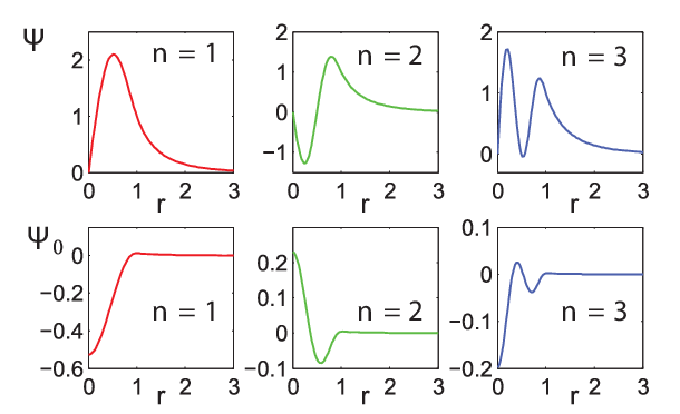
Equation (35) has an infinite set of roots $k_{n}$, $n=1,2\dots$ for each $\varkappa$. Therefore, Eqs. (37), (38) and (39) present the infinite set of solutions with $k=k_{n}$. The solution with $n=1$ (the ground state modon) has no radial nodes. The higher states have $n-1$ nodes (in the interior region). The functions $\Psi_{0}(r)$ and $\Psi(r)$ for the lowest states with $n=1,2,3$ are plotted in Fig 1.

Further we consider only the ground state modon with $k=k_{1}$.

The modon energy $E$ and enstrophy $K$ can be computed straightforwardly

$$E=E_{0}+E_{1},\,\,K=K_{0}+K_{1},$$

(43)

where $E_{0}$ and $K_{0}$ are the energy and enstrophy of the radially symmetric part respectively

$$E_{0}=\frac{2\pi p^{2}a^{5}}{\delta^{2}\varkappa^{2}k^{2}(\varkappa^{2}+k^{2})}\left[\delta^{2}\varkappa^{2}k^{2}+a^{2}(5\delta+1)\right],$$

(44)

	$$\displaystyle K_{0}=\frac{4\pi p^{2}a^{3}}{\delta^{2}(\varkappa^{2}+k^{2})^{2}}\left\{\frac{\delta^{2}}{2}\left[a^{2}(k^{2}-\varkappa^{2})+\varkappa^{4}+k^{4}\right]\right.$$		(45)
	$$\displaystyle\left.+(5\delta+1)\left(a^{2}-\frac{\varkappa^{2}}{2}-\frac{k^{2}}{2}\right)+6\left(1-\frac{a^{2}}{\varkappa^{2}}\right)\right\},$$

and

$$E_{1}=\frac{4\pi}{15}u^{2}a^{5}(1+\mu^{2})\left(1+\frac{\varkappa^{2}}{k^{2}}\right)\left[\delta^{2}\varkappa^{2}+(5\delta+1)\left(\frac{7\varkappa^{2}}{5k^{2}}+\frac{2}{5}-\frac{v_{d}}{u}\right)\right],$$

(46)

$$K_{1}=\frac{2\pi}{3}u^{2}a^{3}(1+\mu^{2})\varkappa^{2}\left(1+\frac{\varkappa^{2}}{k^{2}}\right)\left[\left(\frac{\delta\varkappa k}{a}\right)^{2}+5\delta+1\right],$$

(47)

In dimensional variables (18) one can see that the 3D modon structure is flattened in a plane perpendicular to the direction of the external magnetic field ($xy$ plane) with asymmetry factor $\rho_{s}/R\equiv\omega_{pi}/\Omega_{i}\gg 1$.

In this section, we study the time evolution of the modons under their collisions. To this end, we numerically solve the nonlinear equation (19) with the initial conditions given by a superposition of exact analytical modon solutions (37),i.e.

$$\Phi(\mathbf{r},t)=\Phi_{mod}(\mathbf{r}-\mathbf{r}_{1},t)+\Phi_{mod}(\mathbf{r}-\mathbf{r}_{2},t)$$

(48)

at the time $t=0$. The time integration is performed by an implicit Adams-Moulton method with the variable timestep and the variable order, and local error control. The periodic boundary conditions are assumed. The linear terms are computed in spectral space. The Poisson bracket nonlinearity is evaluated in physical space by a finite difference method, using the energy and enstrophy conserving Arakawa scheme [14]. Total energy and enstrophy were conserved with a relative accuracy less than $5\times 10^{-4}$ during the simulations.

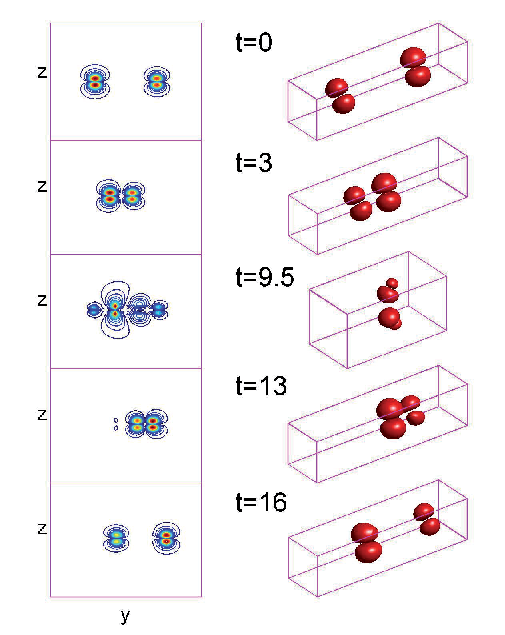
As a first case we consider a collision between the modons which move in opposite directions along the $y$-axis (the head-on collision). The collision is assumed to be with the zero impact parameter, i.e. $x_{1}=x_{2}$, $z_{1}=z_{2}$. The parameter $v_{d}$ is set to $v_{d}=0.1$ in all simulations. The modon velocities are $u_{1}=0.3$ and $u_{2}=-0.5$, and the modon radiuses are $a_{1}=a_{2}=0.5$. The modons are considered to be without radially symmetric and $z$-antisymmetric components, that is $p_{1}=p_{2}=\mu_{1}=\mu_{2}=0$. The time evolution of modons is presented in Fig. 2.

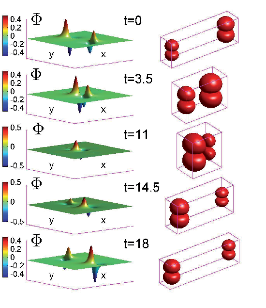
The modons approach each other, $t=3.5$, and undergo a complicated interaction with strong overlapping during the collision, $t=11$, thus generating strong mutual disturbances, as shown at various time intervals in Fig. 2. They then pass through each other and begin to separate, $t=14.5$, and, after all, fully reconstructing their initial form without any emitting wakes of radiation, $t=18$.

The second example is a collision when two modons (without radially symmetric and $z$-antisymmetric components) move in the same direction along the $y$-axis (the overtaking collision). The zero impact parameter collision is also assumed. The modon velocities are essentially different with $u_{1}=-0.3$, $u_{2}=-0.01$ and the modon radiuses are different with $a_{1}=0.5$, $a_{2}=2$. The time evolution is presented in Fig. 3.

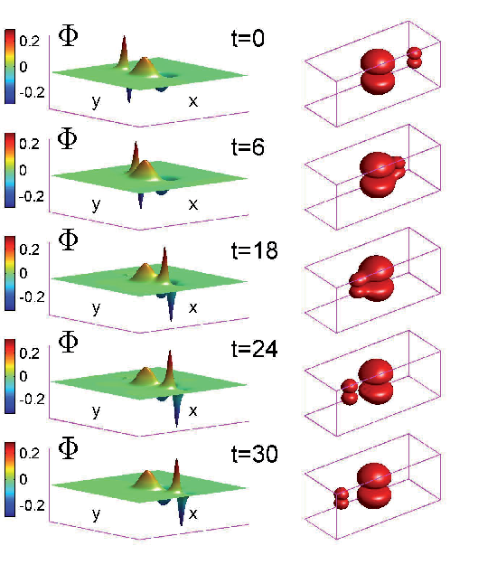
The fast modon catches up with the the slow one, $t=6$, then the modons overlap and pass through each other,$t=18$,begin to separate, $t=24$, and recover their shape, $t=30$. The simulations have been performed for various values of modon velocities and radiuses. Thus, for the 3D modons without radially symmetric and $z$-antisymmetric parts the collisions are elastic for both the head-on and overtaking cases (for the zero impact parameter). Such behavior resembles collisions between one-dimensional solitons in completely integrable models like the NLS and the KdV. The nonzero impact parameter head-on collisions as well as overtaking ones turn out to be inelastic. The modons are destroyed during the course of collision, though for the small impact parameter (compared to modon radiuses) the modons pass through each other almost without changing their shape leaving wakes of radiation, but after all, are destroyed.

Next, we address collisions between modons with radially symmetric ($p_{1}\neq 0$,$p_{2}\neq 0$) or/and $z$-antisymmetric ($\mu_{1}\neq 0$,$\mu_{2}\neq 0$) parts. In this connection, it is necessary to stress that the nonlinearity in Eq. (19) is identically zero for any field distributions with only radial symmetry or/and antisymmetry with the respect to the $z$-axis. Hence, the terms with $p\neq 0$ and/or $\mu\neq 0$ in the solution (37) should be considered as nonlinear perturbations, though the corresponding amplitudes can be much greater than the amplitude of the $x$-antisymmetric component. The head-on collisions with zero impact parameter are considered. The modon parameters are the same as in the case of modons without radially symmetric and $z$-antisymmetric components. Time evolution of modons with radially symmetric parts,$p_{1}=2.$ and $p_{2}=0.3$, is presented in Fig. 4.

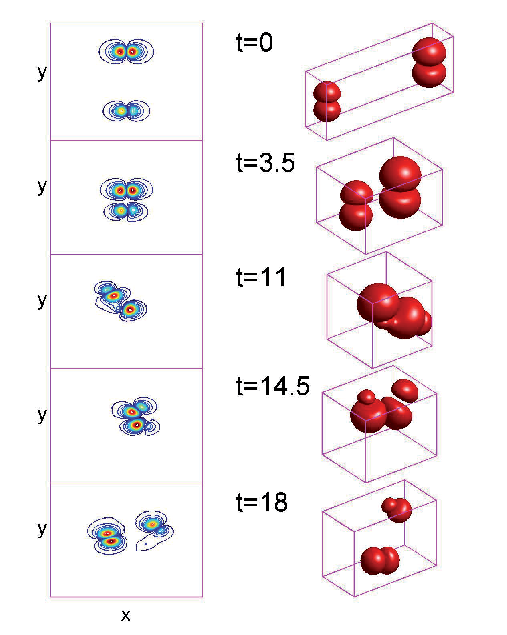
It is seen that after approaching each other, $t=3.5$, and overlapping, $t=11$, the modons propagate in a direction almost perpendicular to the initial direction of propagation and are destroyed during the course of collision, $t=14.5$ and $t=18$.

Inelastic collision of the modons with $z$-antisymmetric part, $\mu_{1}=1.$ (i.e.,the amplitudes of $x$-antisymmetric and $z$-antisymmetric parts are equal) and $\mu_{2}=0.5$ is shown in Fig. 5.

In this case the modons almost preserve their initial shape after collision, $t=16$, resulting in a slightly decreasing the modon amplitudes, but are destroyed at large times (not shown here) due to energy and enstrophy loss connected with emitted radiation. Modons with sufficiently large amplitudes of $x$-antisymmetric parts, $\mu_{1,2}\gg 1$, are fully destroyed immediately after the collision.

We have derived the nonlinear equations that describe coupled drift waves and ion acoustic waves in a plasma assuming electron adiabaticity and negligible ion pressure. We have shown that when the coupling to ion acoustic waves is negligible, the reduced equation is a generalization of the H-M equation to the 3D case. We have found an exact analytical solution of this equation in the form 3D solitary nonlinear drift wave (3D modon). We have performed numerical simulations to study the stability of modons under collisions. The simulations show that the modons without radially symmetric and $z$-antisymmetric parts preserve their shape after the zero-impact parameter collisions (fully elastic soliton collisions) and there is no emitted radiation. This is true for both head-on and overtaking collisions. The modons with radially symmetric or/and $z$-antisymmetric parts are destroyed after collisions. The nonzero-impact parameter collisions between modons are inelastic.

The question of the stability of modons with respect to arbitrary perturbations is still open. The stability properties of the 2D modons was investigated in Ref. [16] (the 2D modons with $v>v_{d}$ are always unstable because of the tilt instability, while the modons with $v<0$ may be stable for some region of parameters). However, as is well known, the stability of soliton structures depends strongly on the dimensionality of space (see, for example, Ref. [17]). The stability of the 3D modons will be discussed in a forthcoming publication.

In conclusion we note, that Eq. (19) can be modified straightforwardly by including an additional nonlinearity of the KdV type $\sim\Phi\partial\Phi/\partial y$ taking into account the effect of the electron temperature gradient [18].

References

- [1] V. I. Petviashvili and O. A. Pokhotelov, Solitary Waves in Plasmas and in the Atmosphere (Gordon and Breach, Reading, PA, 1992).
- [2] W. Horton and Y.-H. Ichikawa, Chaos and Structures in Nonlinear Plasmas (World Scientific, Singapore, 1996).
- [3] A. Hasegawa and K. Mima, Phys. Fluids 21, 87 (1978).
- [4] J. G. Charney, Geophys. Public. Kosjones Nors. Videnshap.- Akad. Oslo 17, 3 (1948)
- [5] V. D. Larichev and G. M. Reznik, Oceanology 16, 547 (1976).
- [6] S. P. Novikov, S. V. Manakov, L. P. Pitaevski, and V. E. Zakharov, Theory of Solitons: The Inverse Scattering Method (Consultants Bureau, New York, 1984).
- [7] M. J. Ablowitz and H. Segur, Solitons and the Inverse Scattering Transform (SIAM, Philadelphia, 1981).
- [8] M. Makino, T. Kamimura, and T. Taniuti, J. Phys. Soc. Jpn. 50, 980 (1981).
- [9] J. C. McWilliams and N. J. Zabusky, Geophys. Astrophys. Dynam. 19, 207 (1982).
- [10] J. D. Meiss and W. Horton, Phys. Fluids 26, 990 (1983).
- [11] J.Pedlosky, Geophysical Fluid Dynamics (Springer-Verlag, Berlin, 1979).
- [12] A. L. Berestov, Izv. Akad. Sci. USSR, Atmos. Oceanic Phys. 15, 443 (1979).
- [13] A. L. Berestov, Izv. Akad. Sci. USSR, Atmos. Oceanic Phys. 17, 60 (1981).
- [14] A. Arakawa, J. Comput. Phys. 1, 119 (1966).
- [15] V. E. Zakharov and E. I. Schulman, Physica D 29, 283 (1988).
- [16] G. E. Swaters, Stud. Appl. Math. 112, 235 (2004).
- [17] Yu. S. Kivshar and G. P. Agrawal , Optical Solitons: From Fibers to Photonic Crystals (Academic, San Diego, 2003).
- [18] X. N. Su, W. Horton, and P. J. Morrison, Phys. Fluids. B 4, 1238 (1992).