Resolving Combinatorial Ambiguities in Dilepton Event Topologies with Constrained Variables
Abstract
We advocate the use of on-shell constrained variables in order to mitigate the combinatorial problem in SUSY-like events with two invisible particles at the LHC. We show that in comparison to other approaches in the literature, the constrained variables provide superior ansatze for the unmeasured invisible momenta and therefore can be usefully applied to discriminate combinatorial ambiguities. We illustrate our procedure with the example of dilepton events. We critically review the existing methods based on the Cambridge variable and MAOS-reconstruction of invisible momenta, and show that their algorithm can be simplified without loss of sensitivity, due to a perfect correlation between events with complex solutions for the invisible momenta and events exhibiting a kinematic endpoint violation. Then we demonstrate that the efficiency for selecting the correct partition is further improved by utilizing the variables instead. Finally, we also consider the general case when the underlying mass spectrum is unknown, and no kinematic endpoint information is available.
1 Introduction
Events with missing transverse energy11 1 is an unfortunate misnomer which stands for the magnitude of the missing transverse momentum . () are arguably the most exciting class of events at the Large Hadron Collider (LHC). They offer the tantalizing possibility of discovering the elusive dark matter — if dark matter particles were produced in the LHC collisions, they would leave the detector without a trace, and the only sign of their presence would be the imbalance in the total transverse momentum of the event. Unfortunately, events with are also notoriously difficult to interpret and analyze:
- •
Instrumental effects. Since the missing transverse momentum is measured only as the recoil against all other visible objects in the event, it can be easily faked by mismeasurement and the finite detector resolution [1]. This problem becomes more severe if the signature involves QCD jets, whose energies and momenta are poorly measured in comparison to leptons and photons.
- •
Unknown nature of the invisible particles. A priori, we do not know the nature of the invisible particles — they could be new particles, or simply the Standard Model (SM) neutrinos [2].
- •
The first step in the analysis of any sample of events is to hypothesize a certain event topology, and design suitable variables adapted to this interpretation [8]. It is already at this stage that one is facing a combinatorial problem, namely, how to associate the various reconstructed objects in the event to the elementary particles in the final state of the event topology. Only in very special cases does the problem not arise — if the event topology is very simple and/or all final state particles are distinct. In general, a typical event at the LHC does suffer from a combinatorics problem, for the following two reasons:
- •
At hadron colliders like the LHC, strong production of colored particles is the dominant production mechanism. When those colored particles decay to the invisible dark matter candidates, the color is shed in the form of QCD jets, which can be confused with jets from initial state radiation (ISR) [9, 10, 11, 12]. In fact, the ISR combinatorics problem is very general and affects any multijet events at hadron colliders, regardless of the presence of in the event.
- •
The lifetime of the dark matter particles is typically protected by some new symmetry. This is often chosen to be a discrete parity, under which the SM particles are even, while the new physics particles are odd. In that case, the new particles are necessarily pair produced, so that each event contains two independent decay chains. This creates a partitioning ambiguity, since the experimenter has to decide whether to assign each reconstructed object to the first or the second decay chain [13]. Wrong assignments would tend to wash out the desired kinematic features and degrade the measurements.
In principle, the combinatorial problem can be addressed in two different ways:
- •
Sidestep the combinatorial problem. The idea here is to design the analysis in such a way that the combinatorial problem does not become an issue. Two possibilities are:
- –
Use global inclusive variables which do not suffer from a combinatorics problem. These variables treat the event as a whole and thus do not depend on the exact event topology, and the combinatorics problem does not arise in the first place. Some well known examples are [14, 15], [16], [17], etc. The disadvantage is that such variables are suboptimal when compared to more exclusive variables which take advantage of the individual characteristics of the event topology.
- –
Use variables which optimize over all possible combinatorial assignments. In this case, instead of trying to figure out the correct assignment in a given event, one considers all possibilities, then chooses the one22 2 The chosen option does not necessarily have to be the correct one. which preserves the relevant useful property of the kinematic variable used in the analysis. As an example, consider an attempt to measure the upper kinematic endpoint of some relevant distribution, such as a two-body invariant mass or the Cambridge variable [18]. One could simply compute the value of the variable under all possible assignments, then choose the smallest among them to be used in the analysis [14, 19, 20, 21, 22, 23, 24, 25, 26, 27].33 3 A similar idea can be applied to measure a lower kinematic endpoint — in that case one would choose the largest value among all possibilities. While this procedure is guaranteed to preserve the kinematic endpoint, it also adversely distorts the shape of the kinematic distribution in the vicinity of the endpoint, making it more difficult to observe in the presence of SM background.
- –
- •
Resolve the combinatorial problem by choosing the “best” assignment event by event. In this case one tries to design an algorithm which will single out one (or maybe several) among the many possible assignments as the most likely “correct” assignment, then use the value of the kinematic variable obtained with this specific choice. Ideally, the algorithm should return a unique selection, which would be correct 100% of the time. Unfortunately, this is rarely achievable in practice, and an important measure quantifying the success of the algorithm is the purity of the resulting sample, i.e., the fraction of events in which the combinatorics was successfully resolved. In principle, there can be different approaches to designing such an algorithm, from the use of a single exclusive variable to a multivariate technique like a neural network analysis [28]. For example, depending on the process at hand, one can attempt to tag ISR jets by a suitable combination of cuts on the jet rapidity and transverse momentum [29] or on the invariant mass and [30]. The partitioning problem into two decay chains is usually addressed by the so-called “hemisphere” algorithm, developed originally within CMS [31] and later adopted in many phenomenological studies [32, 33, 34]. There have been attempts to further improve on the hemisphere algorithm by suitable cuts on the invariant mass and either the jet [35] or [36], by excluding certain reconstructed objects from the clustering algorithm [21, 37], or by recursive jigsaw reconstruction [38]. In general, methods which invoke fewer assumptions, are robust and model independent, but lead to rather vague conclusions, while methods with more assumptions give better results, but are not generally applicable.
In the case of events, the combinatorics problem is exacerbated by the fact that the momenta of the invisible particles are unknown. If the decay chains are sufficiently long, so that there are enough kinematic constraints, one can attempt to compute the individual invisible particle momenta on an event per event basis [39, 40, 41, 42, 43]. Unfortunately, this procedure itself suffers from a combinatorics problem, which only becomes worse as the decay chains get longer (as required for the method to work). For shorter decay chains, like the ones considered in this paper, the method does not apply.
Since the invisible momenta cannot be reconstructed exactly, the next best thing to do is to use some sort of an approximation for them [44]. Again, different approaches are possible. For example, one could use a matrix element method (MEM) to select the most likely values of the invisible momenta. However, the MEM itself suffers from combinatorics, and is rather model dependent since it requires us to fully specify the underlying physics. A better approach would be to rely only on kinematics and obtain the invisible momenta by optimizing a suitable kinematic function. But what constitutes a good target function for such optimization? Initially, the focus was placed on transverse mass variables like [18, 45] and its variants [46, 47, 48, 49]. While transverse quantities are Lorentz invariant under longitudinal boosts, they only provide an ansatz for the transverse components of the individual invisible momenta, and one still needs to provide a supplementary procedure for calculating the longitudinal components of the invisible momenta. One such complementary technique is the MAOS44 4 MAOS stands for -Assisted On-Shell reconstruction. reconstruction [50], where one imposes an additional on-shell kinematic constraint which can be solved for the longitudinal momentum component of each invisible particle. It has been shown that the MAOS approach provides a reasonably good approximation to the true values of the invisible momenta, and can be usefully applied for mass and spin measurements [50, 51, 52]. The MAOS technique was then used to design a novel algorithm [53] for resolving the combinatorial ambiguity in dilepton events, further expanding on the ideas from Refs. [35, 36]. The algorithm aims to resolve the two-fold55 5 In the case of dilepton events, the two jets originating from the top decays can be distinguished from ISR jets by b-tagging. ambiguity in selecting the correct lepton-jet pairing and involves the following three steps:
- •
Step I. Following the proposal of Ref. [36], some number of wrong lepton-jet combinations can be eliminated if they violate the expected endpoints in the distributions of the invariant mass and .
- •
Step II. Utilizing the ansatz found in Step I for the transverse components of the invisible momenta, attempt a MAOS reconstruction of the longitudinal components in two cases:
- 1.
using the known value of the top quark mass ;
- 2.
using the known value of the -boson mass .
Eliminate additional wrong combinations if the solutions for the longitudinal momenta in either case turn out to be complex.
- 1.
- •
Step III. In this final step, one uses the reconstructed masses for the -boson (in case II.1) and the top quark (in case II.2) in conjunction with to decide which of the two lepton-jet pairings is the likelier one.
While this algorithm was originally designed to handle the two-fold ambiguity in events, where the mass spectrum is known, with suitable modifications it can also be applied to new physics searches, as advertised in Ref. [53]. For instance, in the MAOS reconstruction Step II, instead of using the fixed values of the known masses and , one could use the measured endpoints in the respective subsystems [46].
Recently it has been pointed out that the approach has a -dimensional analogue in terms of a general class of on-shell constrained invariant mass variables [8, 54, 55]. Compared to , the variables have several advantages:
- •
- •
Unlike the case of , the optimization procedure required to compute the value of automatically provides an ansatz for both the transverse and the longitudinal components of the invisible momenta. In this sense, once one commits to using variables instead of , the MAOS reconstruction step for finding the longitudinal momentum components is unnecessary.
- •
The maximally constrained variable can be expected to provide the best possible ansatz for the individual invisible momenta, since it takes into account all relevant kinematic constraints in a given event topology [44].
The main goal of this paper is to utilize these advantages of the variables and design an improved algorithm for resolving the combinatorial ambiguity in SUSY-like events with two invisible particles at the LHC. As our benchmark, we shall use the current state of the art algorithm which was proposed and tested for dilepton events in Ref. [53]. Correspondingly, in section 2 we shall first give a brief review of the relevant background information regarding the kinematics of the dilepton event topology. Then in section 3 we shall carefully define the different options for kinematic reconstruction of the invisible momenta [44]. We shall see that in principle there can be different ways of applying the ideas of MAOS reconstruction, -assisted reconstruction, or some combination of both. In section 3 we shall also compare the accuracy of several representative methods for invisible momentum reconstruction.
The next three sections will be devoted to the issue of resolving the combinatorial ambiguity. First in section 4 we critically review each of the three steps of the current state of the art method based on the Cambridge variable and MAOS-reconstruction of invisible momenta [36, 53]. Our goal will be to improve the algorithm in two aspects:
- •
Better performance. By considering various modifications, e.g., utilizing the alternative set of variables, or alternative implementations of the MAOS method itself, we shall attempt to improve the efficiency66 6 Throughout the paper, we shall use the terms “efficiency” and “purity” interchangeably to denote the same quantity — the fraction of events in which the algorithm is successful in identifying the correct partition. of the algorithm in selecting the correct partition in dilepton events.
- •
Simplicity. At the same time, we shall keep an eye on the relative performance of each algorithm component, and if we find components which underperform, we shall eliminate them from consideration, thus simplifying the algorithm. For example, in section 4.2 we shall demonstrate that Step II can be safely disregarded since it is fully correlated with Step I and does not give anything new.
Then in section 5 we consider several new ideas which go beyond the three steps of the current algorithm. In section 5.1 we consider expanding the set of variables used in Step I from two to three, since the dilepton event topology allows not just two, but three independent kinematic endpoints [46, 57]. Then in section 5.2 we discuss a special class of maximally constrained variables where the knowledge of the top and -boson masses can be taken into account already during the optimization stage77 7 Note that this is impossible in the case of purely transverse variables like ., thus further improving the ansatz for the transverse invisible momenta. In section 5.3 we study the potential benefit from using a global inclusive variable such as or an angular variable such as the scattering angle of the parents in the center-of-mass frame. Finally, in section 6 we treat the general case when the underlying mass spectrum is unknown, and no kinematic endpoint information is available. We consider a simplified version of the algorithm which is suitably adapted to this scenario, and investigate its performance in the general new physics mass parameter space. We discuss future extensions of this work and summarize in section 7.
2 Dilepton kinematics and mass-constraining variables
In this section we shall introduce the basic notation and review the relevant class of mass-constraining variables which will be used later to obtain suitable ansatze for the invisible momenta. For the most part, we shall stick to the notation and terminology of Refs. [44, 55]. Following [36, 53], we focus primarily on the “dilepton ” event topology depicted in Fig. 1. This choice is motivated by several factors:
- •
As far as the combinatorial problem is concerned, this is the simplest example which is not trivial — if we were to consider a single-step two-body decay on each side, there would be no combinatorial issue to begin with, and if we were to consider longer decay chains, the problem would become more difficult.
- •
- •

Thus the general event topology considered in this paper is the pair-production of two identical parent particles , followed by a 2-step 2-body decay for each one (see Fig. 1):
| (1) |
In principle, , and should be thought of as some unknown BSM particles, while and are SM particles whose four-momenta are measured. The particles are invisible in the detector, and their momenta are constrained only by the measurement and their (a priori unknown) masses, , with .
The 2-step 2-body event topology of Fig. 1 allows for three different subsystems, as indicated by the colored rectangular boxes [46]. Each subsystem is labelled by the visible particles in it, and defined by a choice of parent and daughter particles, leaving the third type of particles as “relatives”: in subsystem the parents are , the daughters are and the relatives are ; in subsystem the parents are , the daughters are and the relatives are , while in subsystem the parents are , the daughters are and the relatives are . The mass-constraining kinematic variables defined below can be applied to any of the three subsystems, thus each variable has three different versions, depending on the chosen subsystem. For simplicity, in what follows we shall assume that the event topology of Fig. 1 is symmetric, i.e., , , and (see [47, 48] for generalizing to the asymmetric case).
We first consider the traditional transverse variable [18]. Let the two transverse masses of the parent particles be , where is the transverse momentum of and is a test mass for the daughter particles, which is for the case of subsystems and and for the case of subsystem . The kinematic variable is now defined as the absolute minimum of the larger of these two transverse masses, with respect to all possible partitions of the individual invisible transverse momenta ,
| (2) | |||||
Alternatively, one could apply the same procedure to the actual parent masses, , and define the (3+1)-dimensional analogue of Eq. (2) as
| (3) | |||||
where now the minimization is performed over the 3-component momentum vectors and [8]. As shown in Refs. [56, 8, 55], at this point the two definitions (2) and (3) are equivalent, in the sense that the resulting two variables, and , will have the same numerical value.
The case when begins to differ from is when we start to apply additional kinematic constraints beyond the condition . Then the variable can be further refined and one can obtain non-trivial variations [55]:
| (4) | |||||
| (5) | |||||
| (6) | |||||
| (7) | |||||
Here () is the reconstructed mass of the parent (relative) particle in the -th decay chain during the associated minimization procedure and a subscript “” indicates that an equal mass constraint is applied for the two parents (when “” is in the first position) or for the relatives (when “” is in the second position). A subscript “” simply means that no such constraint is applied. In any given subsystem, the variables (2-7) are related event-by-event in the following way [55]
| (8) |
Until now, we have treated the event topology of Fig. 1 in very general terms. In particular, we have not made any assumptions about the nature of the visible particles and . If they are all indistinguishable, e.g., jets from gluino pair-production events, , the resulting combinatorial issues are rather severe, and one should perhaps first focus on testing the hypothesis for the event topology [22]. Here we would like to start with a more tractable problem, where some of the final state particles are distinguishable. Keeping in mind the dilepton example and the analogous BSM signatures, we shall take particles to be -jets, and particles to be leptons, i.e., , , and , where and is the bottom quark. Since the charge of the -jet is difficult to determine, there is a two-fold partitioning ambiguity: the correct partition is
| (9) |
while the wrong partition is
| (10) |
In the rest of this paper, we shall be concerned with designing algorithms which would preferentially select the correct pairing (9) over the wrong one (10). For this purpose, we shall mostly utilize the Cambridge variable (2) and the constrained variable (7). Each of these two variables can be applied to one of the three possible subsystems, , and . Notice, however, that in the “smaller” subsystems and , the two partitions (9) and (10) give identical values of , thus the corresponding subsystem variables and will not be useful to us for the purposes of resolving the combinatorial issue. In contrast, all three subsystem variables, , , and , depend on the partitioning — either directly, or through the relative constraint .
Recently, Ref. [44] introduced another interesting variation of the variable, which takes advantage of the potentially known mass for a relative particle. For example, if the mass of the particles is known, we can enforce it as an additional constraint during the minimization in the subsystem. Specifying to the case, where are the top quarks and are the -bosons , we can write
| (11) | |||||
where is the experimentally measured -boson mass. Similarly, if we take the mass of the top quarks to be known, there is a new variable in the subsystem:
| (12) | |||||
3 Reconstruction schemes for invisible momenta
All of the kinematic variables introduced in the previous section are defined in terms of an optimization procedure over all possible values of the individual invisible momenta. The procedure then singles out one particular choice of the invisible momenta, which is used to calculate the corresponding variable. We can also use this choice as a useful ansatz for the invisible momenta, and then apply standard analysis techniques as if the momenta of the invisible particles were known [50, 44].
The two main goals of this section are:
- •
to list systematically the different ways in which the variables from the previous section can be used (sometimes in combination) to obtain an ansatz for the invisible momenta (see Table 1);
- •
The ansatz for the invisible momenta is generally obtained in two steps88 8 In all cases, one must specify a test mass for the lightest particle (the neutrino in the case of dilepton events.:
- 1.
Fixing the transverse components of the invisible momenta. In principle, there are several possible options here: one can use either an variable, or an variable, which can then be applied to any of the three possible subsystems in Fig. 1. In addition, if one wished to use the mass information for a relative particle, one could also consider the maximally constrained variables (11) and (12). The four columns of Table 1 list four representative examples, illustrating both the use of different variables ( versus ) and the use of different subsystems ( versus ).
Schemes for fixing the components of the invisible momenta longitudinal transverse input MAOS1(;) MAOS4(;) CMAOS1(;) CMAOS4(;) MAOS4(;) MAOS1(;) CMAOS4(;) CMAOS1(;) MAOS2(;) MAOS2(;) CMAOS2(;) CMAOS2(;) MAOS2(;) MAOS2(;) CMAOS2(;) CMAOS2(;) MAOS3(;) MAOS3(;) CMAOS3(;) CMAOS3(;) MAOS3(;) MAOS3(;) CMAOS3(;) CMAOS3(;) — — M2A() — — — — M2A() Table 1: Various methods for reconstructing the transverse and longitudinal momenta of invisible particles in the dilepton event topology of Fig. 1. In all cases, one must specify a test mass for the lightest particle (the neutrino), then superscripts and are used to denote respectively the and subsystems of Fig. 1 (or alternatively, the subsystems and in the notation of Ref. [46]). The methods in the yellow (orange) cells will be investigated in detail in Table 9 (Table 11) below. - 2.
Fixing the longitudinal components of the invisible momenta. Having thus determined the transverse invisible components, the second step is to obtain values for the longitudinal components of the invisible momenta. There are several possibilities (refer to Table 1):
- •
Classic MAOS with mass information (MAOS1 and MAOS4). In the original MAOS approach [50], a mass shell constraint for an intermediate resonance is imposed on each side of the event. Following the notation of [44], we shall make the distinction between cases where the resonance is a parent particle (MAOS1) and a relative particle (MAOS4). In the classic MAOS reconstruction, the transverse invisible components are obtained from , but this can be done for one of several possible subsystems, so we need to implement some notation to indicate which subsystem was used. For example, the abbreviation MAOS1(;) in Table 1 implies that the transverse invisible momenta were obtained from , while the longitudinal invisible momenta were computed from the on-shell conditions for the parent particles (thus MAOS1) with mass . Similarly, the abbreviation MAOS4(;) indicates the use of for fixing the transverse invisible momenta, then applying on-shell conditions for the top quarks, which in subsystem are relative particles (thus the name MAOS4). In both MAOS1 and MAOS4, the longitudinal momenta are obtained up to a four-fold ambiguity, as one has to solve a quadratic equation for each decay side.
- •
Classic MAOS without mass information (MAOS2 and MAOS3). There are two other MAOS schemes, which are applicable in the absence of any mass information about the parent or relative particles [63, 64, 51, 65]. In MAOS2 one forces each parent mass to be equal to the computed value, i.e., , , while in MAOS3 one demands that the parent mass be equal to the corresponding transverse parent mass obtained during the calculation: , . Once again, each of these two MAOS schemes can be applied to any of the three possible subsystems [44]. Furthermore, in the previous step 1 we could in principle use a different subsystem for the determination of the transverse invisible components, therefore now we need two subsystem labels to completely define the procedure. We shall employ the notation where the first subsystem label refers to the determination of the transverse invisible momenta, while the second subsystem label refers to the computation of the respective longitudinal components. For example, the abbreviation MAOS3(;) implies that the transverse components were obtained from , and then the longitudinal components were calculated from the MAOS3 condition for the parents in the subsystem, i.e., the top quarks: , . The MAOS3 procedure always results in an unique ansatz, while MAOS2 is unique only for balanced events, i.e., events with ; for unbalanced events, MAOS2 gives exactly two solutions [55].
- •
-assisted invisible momentum reconstruction. Another alternative is to use an variable — recall that the optimization procedure provides an ansatz for the full 3-vectors of the invisible momenta. As indicated in Table 1, such -Assisted reconstructions will be denoted with M2A and will carry a corresponding subsystem label as well.
- •
Hybrid methods. The remaining methods in Table 1 are hybrid in the sense that they rely on a constrained variable for obtaining the transverse components of the invisible momenta and on one of the MAOS methods for the determination of the longitudinal components. We shall call such methods CMAOS for “constrained” MAOS. The rationale for considering these methods is that, as we shall see below, the constrained variables often provide superior ansatze for the transverse invisible momenta. Once again, one can “mix and match” the subsystems, which necessitates the use of two subsystem arguments for the CMAOS procedures listed in Table 1.
- •
Note that Table 1 does not include all logical possibilities — for example, in order to keep the table compact, we did not list the the maximally constrained variables (11) and (12), which represent another M2A option for simultaneously computing the transverse and longitudinal invisible components. One should also distinguish between methods which use additional mass inputs ( or ) and methods which do not — in what follows, we shall be careful to compare the performance of those two categories of methods separately. For example, the methods in the yellow-shaded cells of Table 1 require an additional mass input and as such they will be discussed and contrasted in Table 9 of section 4.3. On the other hand, the orange-shaded cells of Table 1 highlight a few representative methods which do not require additional mass inputs — those methods will be compared separately in Table 11 of section 4.3. Note that the M2A methods from Table 1 do not use extra mass information.


Having defined the different momentum reconstruction schemes, we are now in position to compare their performance. Following [50, 52], we shall first ask, how close each scheme gets to reproducing the actual values for the invisible momenta. Fig. 2 shows a comparison of the true values of the transverse components (left panel) and the longitudinal components (middle and right panels) of the invisible momenta to the corresponding reconstructed values obtained with different methods from Table 1. The left panel in Fig. 2 contains the combined distributions of the transverse momentum differences and resulting from four different transverse momentum reconstruction schemes: (blue dotted line), (red solid line), (green dashed line) and (magenta dashed line). In all four cases, the distributions are peaked at , which indicates that on average all four methods work rather well. We also observe that the distributions for and , which utilize an extra mass input, are more sharply peaked, leading to much smaller errors. Among the two remaining distributions, appears to perform slightly better than .
The middle and right panels of Fig. 2 show similar plots for the longitudinal momentum difference , obtained with various methods for reconstructing the longitudinal invisible momenta: MAOS1(;) (blue dotted line), MAOS4(;) (black dotted line), (green dashed line), (magenta dashed line), M2A() (red solid line), MAOS2(;) (yellow dotted line) and MAOS3(;) (cyan dashed line). Among the methods requiring an additional mass input (middle panel), and again work best, while among the more conservative methods (right panel), M2A appears to outperform MAOS2 and MAOS3 (see also [44]).


Figs. 3 and 4 provide a more detailed view of the results from Fig. 2 by showing the correlations between and (left panels) and between the difference in magnitudes and the direction mismatch (right panels).


Figs. 3 and 4 reveal that in general, the transverse components of the invisible momenta are reconstructed more accurately than the longitudinal components, and that having additional mass information at one’s disposal definitely helps. The right panels of Fig. 4 also show that for those methods, it is more likely to underestimate (than to overestimate) the magnitude of the invisible momentum — this is easy to understand for the case of events in which the two transverse invisible momenta partially cancel each other out in the sum.
In conclusion of this section, we note that it is known that the performance of the methods with respect to invisible momentum reconstruction can be further improved by selecting only events near the kinematic endpoint of the respective invariant mass variable from which the ansatz originated [50, 44]. However, this benefit comes with a significant loss in statistics, and we shall not pursue this idea further here.
4 Critical review of the standard method
In this section, we analyze the standard method outlined in Refs. [36, 53] for resolving the combinatorics problem in dilepton events. The method involves three steps, which were briefly reviewed in the Introduction, and will be now examined in detail in the following three subsections. For our numerical studies, we generate a partonic dilepton sample with 50k events, using the MadGraph5_aMC@NLO framework at the LHC with TeV center of mass energy and the default set of parton distribution functions [66]. The masses of the top quark and the -boson are set to 173 GeV and 80.419 GeV, respectively, and we also take into account the proper finite widths — as we shall see below, this leads to the presence of events for which the top quarks and/or the -bosons can be significantly off-shell. In order to reduce the background, we apply the same basic cuts as those used in Ref. [53]. This leaves us with 18,456 events after cuts, for a cut efficiency of 37%. The different versions of the and kinematic variables will be computed with the OPTIMASS package [67].
4.1 Step I: and cuts
The first step of the algorithm relies on the fact that in the event topology of Fig. 1, there exist several invariant mass variables, whose distributions exhibit an upper kinematic endpoint. If we choose the correct partition (9), all of these endpoints should be satisfied (barring off-shell effects). On the other hand, the wrong partition (10) may lead to one (or more) endpoint violations. The art of designing a good method for resolving the combinatorics lies in choosing the optimal invariant mass variables which will maximize the number of events for which the wrong partition (10) results in endpoint violations.
In principle, there are two types of invariant mass variables which can have kinematic endpoints:
- •
Using visible particles from the same decay chain. One can study the invariant mass of a collection of visible particles emerging from the same decay chain. For a long decay chain, there are many possible combinations [25], but for a short decay chain like the one in Fig. 1, the choice is unique - we can only form the two-body invariant mass of the -jet and the lepton on each side. This gives us two values, and , each of which should obey the kinematic endpoint , as illustrated in the left panel of Fig. 5.


Figure 5: The distribution of (left), (middle) and (right) for the correct partition (9) (solid lines) and the wrong partition (10) (dotted lines). The inserts show a wider range of the -axis and use a log scale for the -axis. The corresponding and distributions for the and subsystems are shown in Fig. 9 below. Following Refs. [36, 53], we shall apply the stronger condition that the larger of these two values should also obey the upper kinematic endpoint:
(13) where , and are respectively the masses of the top quark, the -boson and the neutrino (we neglect the masses of the -quark and the lepton). With their nominal values from the standard model, the endpoint is located at GeV (see the insert in the left panel of Fig. 5).
- •
Using visible particles from both decay chains. The other possibility is to use the measured momenta of visible particles from both decay chains in order to construct invariant mass variables which also exhibit upper kinematic endpoints [8]. The prototypical example of such a variable is the Cambridge variable (see the middle panel in Fig. 5), but there are other possibilities as well, e.g., [68, 69], [70], and more recently, [55] (see the right panel in Fig. 5). Following Refs. [36, 53], we shall continue to consider , but we shall also entertain the possibility of using instead. For the correct partition, the distributions of and have common kinematic endpoints, and so the values of and obey the hierarchy
(14) (15) where the endpoint values correspond to using the true99 9 If the neutrino mass were unknown, one could use any arbitrary value for the test daughter particle mass, and then extract the endpoint values in (14) and (15) from the data. value of the neutrino mass . More importantly, for the wrong partition, the shapes of the and distributions are different (compare the blue dotted lines in the middle and right panels of Fig. 5), which will affect the efficiency for selecting the correct partition. Due to the general property (8), the wrong partition will still preserve the hierarchy , and therefore, the chances of endpoint violations will be increased if we were to use in place of [61].
| Quadrant | Quadrant for | |||
|---|---|---|---|---|
| for | I | II | III | IV |
| I | ||||
| II | ||||
| III | ||||
| IV | ||||
The distributions in Fig. 5 clearly motivate the use of the variables and (or perhaps instead) to resolve the two-fold combinatorial ambiguity.1010 10 For now, as in Refs. [36, 53], we shall focus on the subsystem, where one would expect the largest number of endpoint violations for the wrong kinematics [61]. The other two subsystems, and , will be discussed later in section 5.1. This idea is implemented as Step I of the algorithm, by requiring that the invariant mass variables computed with a given partition , obey the two kinematic endpoints (13) and (14). If one of the partitions obeys both endpoints, while the other does not, the former (latter) is declared to be the correct (wrong) partition ().
In order to quantify the discussion in the rest of paper, we introduce a simple Cartesian coordinate system designed to keep track of the kinematic endpoint violations (see Fig. 6). The and variables will be chosen so that their values are positive (negative) in the absence (presence) of a kinematic endpoint violation. To this end, we shall consider the difference between the value of the upper kinematic endpoint and the value of the variable itself — this difference is expected to be positive for the correct partition , and conversely, if the difference is negative, it is likely that we have chosen the wrong partition . Thus in Fig. 6 we choose the -axis to be (later on we shall also consider ), while for the -axis we take , where and are the invariant masses of the two -lepton pairs in a given partition. As usual, the plane in Fig. 6 is divided into four quadrants, labelled I, II, III and IV. With this setup, one would expect that the correct partition will be registered in the first quadrant I, while the wrong partition can end up anywhere, including quadrants II, III and IV, which would indicate some sort of an endpoint violation.


These expectations are confirmed in Fig. 7, which shows scatter plots in the plane of Fig. 6 for events with the correct partition (left panels, red points) and the wrong partition (right panels, blue points). We see that the correct partition mostly populates quadrant I, although there is some leakage into the other three quadrants due to off-shell effects. On the other hand, the wrong partition cases are significantly spread out, and the majority of the events live outside quadrant I. The effect is even more pronounced if we trade for and consider as our -axis variable (see the plots in the bottom row of Fig. 7).
We are now in position to define the action of Step I of the algorithm. For each event, there are two possible partitions, from (9) and from (10). Since we do not know which is which, from now on we shall denote them with , . (It does not matter which partition is labelled first and which is labelled second.) Each partition will produce a point in one of the four quadrants within the plane of Fig. 6. We will then resolve the partitioning ambiguity according to Table 3.
| Quadrant | Quadrant for | |||
|---|---|---|---|---|
| for | I | II | III | IV |
| I | unresolved | |||
| II | unresolved | unresolved | ||
| III | unresolved | |||
| IV | unresolved | unresolved | ||
Whenever one of the two partitions falls in quadrant I while the other does not, then the partition in quadrant I will be declared to be the correct one (). If both partitions fall in the same quadrant, then the event remains “unresolved” at Step I and we need to wait for the next steps of the algorithm. The situation becomes more complicated if both partitions fall outside quadrant I, and within different quadrants. In that case, we shall make the distinction between quadrant III, where both endpoints are violated, and quadrants II and IV, where there is a single endpoint violation. Correspondingly, if one partition falls in quadrant III while the other does not, the partition in quadrant III will be declared as the wrong partition (). Finally, if one partition is in quadrant II while the other in quadrant IV, the event remains unresolved.
As a result of the application of Table 3, each event will fall into one of two categories: resolved, for which one of the partitions has been declared to be correct, and unresolved, for which no decision has been reached at that stage. Furthermore, the resolved events will not always be identified correctly — on occasion, the algorithm will misidentify the wrong partition as being the correct one. In order to better understand the power of each method below, we shall find it convenient to quote our results in the form of tables like Table 2, where we separately keep track of the quadrant for the correct partition (indicated by the row label) and the quadrant for the wrong partition (indicated by the column label). Each event will belong to one of the 16 boxes of Table 2, and we will be interested in the number of events within each box, where the “quadrant indices” (for the correct partition) and (for the wrong partition) take values in the set . The action by Table 3 then causes all events within the green-shaded boxes of Table 2 to be correctly resolved, the events within the red-shaded boxes of Table 2 to be wrongly resolved, while the events within the unshaded boxes of Table 2 to remain unresolved. Then, for any given event sample, the total number of correctly resolved events will be given by the total number of events within the green-shaded boxes of Table 2:
| (16) |
Similarly, the total number of wrongly resolved events will be equal to the total number of events within the red-shaded boxes of Table 2:
| (17) |
Finally, the total number of unresolved events is the sum of all events within the unshaded (white) boxes of Table 2:
| (18) |
The algorithms below will be applied so that once an event is resolved, it does not get reclassified at a later stage, i.e., subsequent steps of the algorithm only affect the remaining unresolved events. Obviously, at different steps of the algorithms, the number of correctly resolved events (), wrongly resolved events () and unresolved events will vary, but those three numbers will always add up to the total number of events in the sample:
| (19) |
In order to compare different algorithms, we define the expected efficiency (sometimes called purity) as
| (20) |
For the purposes of calculating the efficiency, we shall assume that any unresolved events are eventually decided with a coin flip (50% efficiency).
| Quadrant counts based on and | ||||
|---|---|---|---|---|
| Quadrant | Quadrant for | |||
| for | I | II | III | IV |
| I | 6194 | 910 | 9793 | 1020 |
| II | 22 | 31 | 106 | 5 |
| III | 29 | 10 | 191 | 4 |
| IV | 41 | 3 | 91 | 6 |
| Quadrant counts based on and | ||||
|---|---|---|---|---|
| Quadrant | Quadrant for | |||
| for | I | II | III | IV |
| I | 4494 | 2317 | 10222 | 217 |
| II | 168 | 178 | 480 | 5 |
| III | 37 | 26 | 251 | 1 |
| IV | 17 | 3 | 38 | 2 |
Our results for are shown in Table 4, where the quadrants from Fig. 6 have been defined in terms of the variables and (left table) and the variables and (right table). As expected, the most populated entries are found in the first rows, which confirms that in the case of the correct partition , endpoint violations are relatively rare1111 11 As a sanity check, we have verified that if we turn off the width effects by hand, by forcing both the top quarks and the -bosons on-shell, all entries in the second through fourth rows are exactly zero.. We also find a handful of events in the off-diagonal boxes of the first column — for those events, off-shell effects caused the correct partition to violate one or both of the kinematic endpoints, while the wrong partition accidentally happened to satisfy both kinematic endpoints. Such events are problematic since they will be wrongly identified — one should keep in mind that only the symmetric combination of events is experimentally observable, since a priori we do not know which is the correct partition. Nevertheless, we observe that in the cases when one of the partitions ends up in quadrant I while the other does not, the large majority of the events will be correctly identified, since
| (21) |
Another piece of good news is that whenever one of the partitions violates exactly one endpoint, while the other violates both, it is much more likely that the former (latter) is the correct (wrong) partition:
| (22) |
Combining the relations (21) and (22) and using the definitions (16) and (17), we conclude that , and therefore Step I of the method works relatively well1212 12 This can also be seen directly by comparing the green-shaded and the red-shaded boxes of Table 4.. With our definition for the efficiency (20), the classic method based on and gives an efficiency of 82%. Looking back at the left side of Table 4, we see that for the standard method, the efficiency is hurt by the relatively large fraction of events which remain unresolved at this stage — the unshaded boxes contain a total of events, or about 35% of the sample. The situation improves somewhat if we use the variable instead of : in that case, the right table of Table 4 contains fewer unresolved events (, or only 27%), while the desired relations (21) and (22) are further enhanced. Both of these effects are responsible for increasing the efficiency (20) of the new method to 85.3%. Note that in both methods, the majority of the unresolved events are found in the very first diagonal box , where both partitions are fully consistent with the kinematics of the assumed event topology. This is why, in what follows we shall focus our attention on the additional steps of the algorithm which can successfully classify the remaining unresolved events, especially those in the box.
4.2 Step II: The presence of complex solutions
In the second step of the method, one attempts to reconstruct the longitudinal momenta of the invisible particles, by enforcing on-shell conditions for a parent particle (MAOS1) or for a relative particle (MAOS4). Since the on-shell conditions result in quadratic equations, the solutions are not guaranteed to be real. The idea of Step II is to compare the two possible partitions in terms of the number of complex solution pairs for the longitudinal momenta. Since there is a separate calculation for each decay chain, there are three possible outcomes:
- •
. Both decay chains result in real solutions.
- •
. Exactly one decay chain gives a pair of complex solutions, while the other decay chain has real solutions.
- •
. Both decay chains result in complex solutions.
For the purposes of applying Step II of the method, there is no need to distinguish between the cases of and , since the important point is simply that . The action of Step II is the following: if one of the partitions gives , while the other has , then the former (latter) partition is declared to be the correct (wrong) one.
| I | II | III | IV | ||||||||||
| 0 | 1 | 2 | 0 | 1 | 2 | 0 | 1 | 2 | 0 | 1 | 2 | ||
| I | 6194 | 0 | 0 | 910 | 0 | 0 | 9793 | 0 | 0 | 1020 | 0 | 0 | |
| 6194 | 0 | 0 | 0 | 1 | 909 | 0 | 7215 | 2578 | 1020 | 0 | 0 | ||
| II | 0 | 2 | 20 | 0 | 0 | 31 | 0 | 2 | 104 | 0 | 0 | 5 | |
| 22 | 0 | 0 | 0 | 0 | 31 | 0 | 69 | 37 | 5 | 0 | 0 | ||
| III | 0 | 22 | 7 | 0 | 5 | 5 | 0 | 124 | 67 | 0 | 4 | 0 | |
| 29 | 0 | 0 | 0 | 0 | 10 | 0 | 138 | 53 | 4 | 0 | 0 | ||
| IV | 41 | 0 | 0 | 3 | 0 | 0 | 91 | 0 | 0 | 6 | 0 | 0 | |
| 41 | 0 | 0 | 0 | 0 | 3 | 0 | 66 | 25 | 6 | 0 | 0 | ||
| I | II | III | IV | ||||||||||
| 0 | 1 | 2 | 0 | 1 | 2 | 0 | 1 | 2 | 0 | 1 | 2 | ||
| I | 5005 | 1086 | 103 | 582 | 299 | 29 | 8245 | 1497 | 51 | 908 | 109 | 3 | |
| 4094 | 2074 | 26 | 136 | 751 | 23 | 3893 | 5817 | 83 | 661 | 359 | 0 | ||
| II | 7 | 14 | 1 | 12 | 16 | 3 | 58 | 46 | 2 | 2 | 3 | 0 | |
| 9 | 13 | 0 | 5 | 24 | 2 | 26 | 79 | 1 | 1 | 4 | 0 | ||
| III | 12 | 17 | 0 | 5 | 5 | 0 | 84 | 106 | 1 | 3 | 1 | 0 | |
| 22 | 7 | 0 | 3 | 6 | 1 | 96 | 95 | 0 | 3 | 1 | 0 | ||
| IV | 36 | 5 | 0 | 3 | 0 | 0 | 78 | 13 | 0 | 6 | 0 | 0 | |
| 31 | 10 | 0 | 1 | 2 | 0 | 58 | 33 | 0 | 6 | 0 | 0 | ||
As already discussed in section 3, there are several ways to implement the MAOS idea and compute longitudinal invisible momenta. Tables 5 and 6 show results for the cases of MAOS1(;) and MAOS4(;), respectively1313 13 The former was the method used in Ref. [53], but the latter is in principle a viable option as well.. Similarly to Table 4, each table is organized by quadrants, and within each cell we show the number of events with a given value of , for the correct partition (upper rows) and the wrong partition (lower rows).
Let us first focus on Table 5, which shows several interesting trends. First, recall the motivation behind Step II — one was hoping to find that the correct partition would always give real solutions (), while the wrong partition would always lead to complex solutions (). Table 5 reveals that this expectation is indeed true, but only for certain quadrant pairs: , , and . For those cases, Step II would be able to perfectly resolve the combinatorial ambiguity, and it seems that the method works as designed. Unfortunately, three out of these four quadrant pairs are already shaded in green (see Table 2), which means that those events were already perfectly resolved by Step I, thus the additional benefit from Step II for those three quadrant pairs is exactly zero. As for the fourth quadrant pair, , it is very sparsely populated, and furthermore, any benefit there would be offset by the negative effects from the symmetric case of , where the results are contrary to our expectations above — now it is the correct partition which leads to complex solutions1414 14 The fact that the correct partition may result in complex momenta should not be surprising — this can be due to finite width and off-shell effects. As a sanity check, we have verified that in the zero-width limit only the first row in Table 5 has any non-zero entries, while the second, third and fourth rows are empty.. (The same phenomenon is observed for the other three symmetric pairs as well — see the red-shaded boxes corresponding to , , and , where it is again the correct partition which has .)
Thus we conclude that for the events which were already resolved at Step I (the green-shaded and red-shaded cells in Table 5), Step II does not bring anything new — its results are either fully correlated with Step I (as for the quadrant pairs , and and their red-shaded symmetric partners on the other side of the diagonal), or inconclusive, since the two partitions behave identically (e.g., for quadrant pairs and and their partners). Therefore, we need to concentrate on the unresolved events in the unshaded cells in Table 5, since those were precisely the events which Step II was meant to address. Unfortunately, we observe that in the unshaded cells along the diagonal in Table 5, the two partitions lead to the same result and cannot be discriminated, while the remaining two cells and were already discussed above — their statistics is too low, and they tend to cancel each other out, thus they will not appreciably affect the overall efficiency.
Based on the results from Table 5, we conclude that if one were to apply Step II based on the MAOS1(;) method, which was used in Ref. [53], there would be no additional benefit beyond Step I, and therefore Step II is unnecessary and can be eliminated. However, this still leaves open the question whether some modified version of Step II can still be useful, e.g., applying a different MAOS scheme like MAOS4(;) (see Table 6), or perhaps using one of the CMAOS schemes based on the variables (see Tables 7 and 8).
| I | II | III | IV | ||||||||||
| 0 | 1 | 2 | 0 | 1 | 2 | 0 | 1 | 2 | 0 | 1 | 2 | ||
| I | 4494 | 0 | 0 | 2317 | 0 | 0 | 10222 | 0 | 0 | 217 | 0 | 0 | |
| 4494 | 0 | 0 | 348 | 729 | 1240 | 62 | 5482 | 4678 | 217 | 0 | 0 | ||
| II | 62 | 70 | 36 | 63 | 64 | 51 | 184 | 168 | 128 | 2 | 1 | 2 | |
| 168 | 0 | 0 | 21 | 53 | 104 | 4 | 211 | 265 | 5 | 0 | 0 | ||
| III | 2 | 20 | 15 | 4 | 9 | 13 | 7 | 138 | 106 | 0 | 1 | 0 | |
| 37 | 0 | 0 | 3 | 7 | 16 | 0 | 150 | 101 | 1 | 0 | 0 | ||
| IV | 17 | 0 | 0 | 3 | 0 | 0 | 38 | 0 | 0 | 2 | 0 | 0 | |
| 17 | 0 | 0 | 0 | 1 | 2 | 0 | 25 | 13 | 2 | 0 | 0 | ||
| I | II | III | IV | ||||||||||
| 0 | 1 | 2 | 0 | 1 | 2 | 0 | 1 | 2 | 0 | 1 | 2 | ||
| I | 3840 | 497 | 157 | 1810 | 385 | 122 | 9089 | 931 | 202 | 214 | 3 | 0 | |
| 3652 | 612 | 230 | 397 | 879 | 1041 | 3005 | 3132 | 4085 | 217 | 0 | 0 | ||
| II | 52 | 66 | 50 | 65 | 84 | 29 | 228 | 194 | 58 | 1 | 2 | 2 | |
| 113 | 37 | 18 | 30 | 81 | 67 | 121 | 143 | 216 | 5 | 0 | 0 | ||
| III | 14 | 13 | 10 | 11 | 9 | 6 | 101 | 76 | 74 | 1 | 0 | 0 | |
| 33 | 3 | 1 | 10 | 11 | 5 | 90 | 88 | 73 | 1 | 0 | 0 | ||
| IV | 17 | 0 | 0 | 3 | 0 | 0 | 38 | 0 | 0 | 2 | 0 | 0 | |
| 17 | 0 | 0 | 1 | 0 | 2 | 18 | 12 | 8 | 2 | 0 | 0 | ||
But before we discuss these options, it will be useful to understand the results from Table 5 from a physics point of view. A careful inspection of Table 5 reveals that its content can be summarized as follows: for any partition , quadrants I and IV produce only real solutions, while quadrants II and III lead to only complex solutions. This means that the existence of complex solutions is correlated with the -axis variable of Fig. 6 (), and not with the -axis variable (). This is easy to understand: is formed from visible particle momenta only, and is not directly related to any invisible momenta. Therefore, a violation of the kinematic endpoint by itself does not imply unphysical invisible momenta. On the other hand, the physical meaning of is the lowest possible mass of the parent particle, in this case the top quark. If the value of strictly violates the kinematic endpoint , i.e., , then enforcing the on-shell condition for the top quark will necessarily result in unphysical (complex) values for the momenta. In particular, quadrants II and III, in which the endpoint is violated by definition, will always produce complex momenta.
While the above logic helps to understand the results from Table 5, it does not carry over directly to the case of MAOS4(;) shown in Table 6, since now we are enforcing an on-shell condition for a different (relative) particle. The trends which we previously observed in Table 5 are still noticeable, but they are not so clear cut. Nevertheless, if we focus on the unresolved events after Step I (the unshaded cells in Table 6), we again see that Step II does not do particularly great on those events. The largest effect is in the cell, where the efficiency for resolving the correct partition is , which is slightly better than a coin flip. Adding up the results from all previously unresolved cells, we find that if we were to perform Step II with the MAOS4(;) version of the method instead of the MAOS1(;) option used in Ref. [53], the overall efficiency would increase to 84.5%, which is still worse than the result (85.3%) found in section 4.1 with the improvements in Step I alone, taking advantage of (see the right table in Table 4).
Tables 7 and 8 show results from two similar exercises where we use the corresponding CMAOS methods, i.e., fixing the transverse components of the invisible momenta from instead of , then applying the on-shell conditions for the parent (top quark) or relative (-boson) particle. As shown previously in Figs. 2-4, the variable generally provides a more accurate estimate of the individual transverse momentum components for the invisible particles, and one might hope that incorporating somehow into the Step II algorithm would improve the performance. However, Table 7 shows that the improvement in the case of CMAOS1(;) is very marginal — the efficiency increases from 85.3% after Step I to 85.4% after Step II. The effect is slightly better in Table 8, which uses the CMAOS4(;) option — there the efficiency increases from 85.3% after Step I to 85.9% after Step II. However, even this increase is too small to justify the presence of Step II — as we shall see later on, there exist other, much more effective techniques. Therefore, as a final summary of this subsection, we conclude that Step II can be safely dropped altogether, since its results are largely correlated with Step I.
4.3 Step III and possible variations
In this subsection we shall discuss different possible options for the third step of the method and investigate their performance. To recap the situation: when we used and at Step I, we ended up with correctly resolved events, incorrectly resolved events, and unresolved events, for an efficiency of 82% (see the top of the middle column in Table 9).
| Algorithm for Step I | ||||||
| and | and | |||||
| Correct | Wrong | Unresolved | Correct | Wrong | Unresolved | |
| Step I: Quadrant counts | 11,920 | 106 | 6,430 | 13,274 | 249 | 4,933 |
| efficiency | ||||||
| Remaining unresolved events | ||||||
| method | 3,445 | 1,573 | 1,412 | 2,820 | 1,462 | 651 |
| cumulative efficiency | ||||||
| type cut alone | 3,160 | 3,270 | — | 2,426 | 2,507 | — |
| cumulative efficiency | ||||||
| and alone | 4,101 | 1,624 | 705 | 2,868 | 1,328 | 737 |
| cumulative efficiency | ||||||
| with MAOS4(;) | 2,392 | 1,371 | 2,667 | 2,212 | 1,238 | 1,483 |
| cumulative efficiency | ||||||
| with MAOS1(;) | 4,186 | 2,188 | 56 | 3,033 | 1,860 | 40 |
| cumulative efficiency | ||||||
| with CMAOS4(;) | 2,262 | 1,307 | 2,861 | 2,122 | 1,228 | 1,583 |
| cumulative efficiency | ||||||
| with CMAOS1(;) | 2,995 | 1,790 | 1,645 | 2,565 | 1,617 | 751 |
| cumulative efficiency | ||||||
| with MAOS1(;) | 4,344 | 1,856 | 230 | 3,044 | 1,546 | 343 |
| cumulative efficiency | ||||||
| with MAOS4(;) | 1,627 | 792 | 4,011 | 1,505 | 760 | 2,688 |
| cumulative efficiency | ||||||
| with CMAOS1(;) | 3,328 | 1,583 | 1,519 | 3,044 | 1,459 | 430 |
| cumulative efficiency | ||||||
| with CMAOS4(;) | 1,922 | 947 | 3,561 | 1,870 | 928 | 2,135 |
| cumulative efficiency | ||||||
If, on the other hand, we choose to use and at Step I, we obtain correctly resolved events, incorrectly resolved events, and unresolved events, for an efficiency of 85.3% (see the top of the right column in Table 9). Then in section 4.2 we showed that Step II does not add much and can be ignored. This brings us to Step III, whose purpose is to further classify the remaining unresolved events after Step I (6,430 and 4,933, respectively) on a statistical basis, using suitable discriminating variables.
We begin by reviewing the method suggested in Ref. [53], which introduced several kinematic variables, , . These variables were designed so that their values tend to be larger for the case of the wrong partition, i.e.
| (23) |
While it is not guaranteed that (23) will be true in every single event, if it holds for the majority of the events, one can attempt to identify the correct partition by declaring [53]
| (24) |
where
| (25) |
In the case of several good variables , one can generalize (24) by choosing the correct partition to be the partition () if the majority of the quantities are positive (negative). In the following, we shall refer to this procedure as the “ method” [53].
The variables considered in Ref. [53] were the following:
| (26) | |||||
| (27) | |||||
| (28) | |||||
| (29) |
where is one of two partitions and the index labels the two decay chains in Fig. 1. The variable () is the reconstructed mass of the top quark (the -boson) with a MAOS-type method which uses the -boson mass (the top mass) as an input. Since the longitudinal invisible momenta are obtained from a quadratic equation, in general there are two solutions, labelled by , corresponding to the two signs in front of the discriminant. Thus in each event one can obtain four reconstructed top quark masses, , and four reconstructed -boson masses, . The idea behind the and variables in (28) and (29) is to compare those reconstructed values to the true values and , respectively. For the correct partition , on average one might expect to find the reconstructed values closer to the true ones, in agreement with (23).
In Table 9 we test several options for discrimination variables which can be applied at Step III. Our benchmark is the method of Ref. [53], which made use of only three variables, , and , since the fourth one, , was found to be significantly correlated with . For consistency, whenever the quadrants from Step I are defined in terms of (right column in Table 9), we shall replace (27) with . Table 9 reports results from both versions of the method — we see that the overall efficiency can be further improved to 87.1% and 89%, respectively. The observed improvement at Step III is due to correctly categorizing (at the rate of about 2:1) the majority of the remaining unresolved events — see Table 10, which gives the breakdown among the individual “unresolved” cases from Table 3.
| Quadrants | Algorithm for Step I | |||||||
| with unresolved | and | and | ||||||
| events | Total | C | W | U | Total | C | W | U |
| (I, I) | 6,194 | 3,266 | 1,521 | 1,407 | 4,494 | 2,471 | 1,308 | 715 |
| (II, II) | 31 | 26 | 5 | - | 178 | 147 | 26 | 5 |
| (III, III) | 191 | 149 | 37 | 5 | 251 | 185 | 55 | 11 |
| (IV, IV) | 6 | 1 | 5 | - | 2 | 0 | 2 | - |
| (II, IV) (IV, II) | 8 | 3 | 5 | - | 8 | 3 | 3 | 2 |
| Total after Step III | 6,430 | 3,445 | 1,573 | 1,412 | 4,933 | 2,820 | 1,462 | 651 |
In spite of this progress, we also notice that a certain number of events (1,412 and 651, correspondingly) still remain unresolved. At first glance, this seems odd, since the method uses an odd number of variables, so for each event, there should be a clear winner between the two candidate partitions and . However, recall that the longitudinal momentum reconstruction sometimes results in complex solutions, in which case the corresponding variable or is undefined.1515 15 This will become more evident when inspecting the normalization of the plots in Fig. 8 below. Thus the remaining unresolved events after Step III are those where only two of the three variables were calculated, and each preferred a different partition .
Table 10 demonstrates that Step III was relatively successful. Nevertheless, in the remainder of this section we shall investigate whether further improvements at the level of Step III are still possible. Let us begin by studying the benefit from each individual variable, , and , used in the algorithm. Following Ref. [53], in Fig. 8 we show distributions of the “ordered” differences
| (30) |
for the three variables (left panels), (middle panels) and (right panels), where we use MC truth information to make sure that we subtract the variables in the order indicated in (30).


For the plots in the top (bottom) row of Fig. 8, the transverse invisible momenta were obtained with the help of the () variable. Plotting in terms of the ordered difference (30) is very useful, since it allows us to see how often the expected relationship (23) holds: the difference (30) is positive (negative) if (23) is satisfied (violated). Thus, by applying the prescription (24) for a given variable , we shall correctly resolve all events with positive values of (the shaded portions of the distributions in Fig. 8), and we shall wrongly resolve the events with negative values of (the unshaded portions of the distributions in Fig. 8). By comparing the areas of the shaded and unshaded portions of each distribution, we can judge the discrimination power of each variable. For example, the left panels in Fig. 8 show that when considering the whole event sample (red histograms), appears to be a good variable, since as many as 79% of the events have positive values of [53]. Unfortunately, we find that this conclusion is invalidated after the application of Step I — for the remaining unresolved events after Step I (the blue histograms in Fig. 8), it is actually more likely to find a negative value of instead, thus obtaining the wrong answer for . This observation reveals that the results from Step I and Step III are also somewhat correlated — the events which are easy to analyze with at Step III would already be correctly resolved at Step I. Using alone (without or ) in fact lowers the cumulative efficiency, as shown in Table 9. This motivates us to drop from further consideration and repeat Step III without , i.e., with only and . As shown in Table 9, this leads to a slight improvement of the cumulative efficiency, to 88.7% and 89.5%, respectively, indicating that and retain some discrimination power even after Step I (this can also be deduced from the blue histograms in the middle and right panels of Fig. 8).
Given the large variety of MAOS and CMAOS methods described in section 3 (see Table 1), next we check if there exist alternative versions of the and variables which are better suited for our purpose. In the remainder of Table 9 we study the effect on the cumulative efficiency if the reconstruction is performed with one of the eight yellow-shaded methods from Table 1. Taking one variable at a time, we apply Step III as in (24) and quote the resulting cumulative efficiency in the last 8 rows of Table 9. The results are rather illuminating, and indicate that “not mixing” the subsystems provides the best option for constructing a useful variable. For example, when the transverse invisible components are fixed with the help of the subsystem, in which the top quark is the parent particle, then we are better off applying the on-shell condition on the same particle in order to reconstruct the longitudinal invisible momenta. Similarly, if the transverse momenta are obtained from the subsystem, in which the -boson is the parent particle, then it is preferable to apply the on-shell condition on the -boson as well. For both MAOS and CMAOS reconstructions, Table 9 shows that the highest efficiencies are obtained in the case of and type variables. It is interesting to note that the performance of the modified method above (which used only and ) can be matched and even slightly exceeded by using a single additional variable at Step III, provided that we pick the right one: the MAOS1(;) option gives 88.8% (compare to 88.7% before), while CMAOS1(;) yields 89.6% (compare to 89.5%).
Another interesting point is that in all cases, the cumulative efficiencies in the right column of Table 9 are higher than those in the middle column, thus reinforcing the idea of using the constrained variables. In section 4.1 we already established that it is beneficial to redefine Step I in terms of variables, and now we see that this advantage is retained after Step III as well.
Finally, one may wonder if there is any additional benefit in combining at Step III two or more of the variables considered in Table 9. We test this idea with the following exercise. Let us revisit Step III, again dropping the variable (27) from consideration, while for the definition of and let us choose the two best performing CMAOS variables from the right column of Table 9, namely with CMAOS1(;) (87.9%) and with CMAOS1(;) (89.6%). In this modified scheme, we obtain a cumulative efficiency of with correctly identified, wrongly identified and unresolved events. Similarly, choosing the two best MAOS options in the middle column of Table 9, namely with MAOS1(;) (87.4%) and with MAOS1(;) (88.8%), we find a final efficiency of (with correctly identified, wrongly identified and unresolved events). In both exercises, the final efficiency is slightly worse than what would be obtained with the single best variable alone, although the number of unresolved events decreased. These two exercises indicate that there exist non-trivial correlations between the different variables and an improvement of the efficiency is not guaranteed by simply merging or combining different methods. This is one of the reasons why we kept the results for the different methods separate in Table 9.
Up to this point, in Steps II and III we have used reconstruction methods which require the knowledge of a particle mass ( or ). However, when the method is being applied in studies of new physics, such information may not be immediately available. Therefore, it is prudent to consider modifications of Steps II and III, where one uses methods from Table 1 which do not rely on any mass information.
| Algorithm for Step I | ||||||
| and | and | |||||
| Correct | Wrong | Unresolved | Correct | Wrong | Unresolved | |
| Step I: Quadrant counts | 11,920 | 106 | 6,430 | 13,274 | 249 | 4,933 |
| efficiency | ||||||
| Remaining unresolved events | ||||||
| with MAOS3(;) | 3,527 | 2,903 | - | 2,980 | 1,953 | - |
| cumulative efficiency | ||||||
| with CMAOS3(;) | 3,657 | 2,773 | - | 2,914 | 2,019 | - |
| cumulative efficiency | ||||||
| with M2A() | 3,495 | 2,935 | - | 2,759 | 2,174 | - |
| cumulative efficiency | ||||||
| with M2A() | 3,719 | 2,711 | - | 2,699 | 2,234 | - |
| cumulative efficiency | ||||||
| with MAOS3(;) | 3,877 | 2,553 | - | 2,783 | 2,150 | - |
| cumulative efficiency | ||||||
| with CMAOS3(;) | 3,628 | 2,802 | - | 2,622 | 2,311 | - |
| cumulative efficiency | ||||||
| with M2A() | 3,769 | 2,661 | - | 2,658 | 2,275 | - |
| cumulative efficiency | ||||||
| with M2A() | 3,448 | 2,982 | - | 2,529 | 2,404 | - |
| cumulative efficiency | ||||||
To be specific, we focus on the four methods listed in the orange-shaded cells of Table 1 and show the corresponding results in Table 11, which is the direct analogue of Table 9. Once again, it turns out that Step II is unnecessary, albeit for a different reason — this time in all cases the solutions for the invisible momenta are found to be real and therefore invisible momentum reconstruction is always possible for both partitions. It also follows that there will be no unresolved events after Step III, since the relevant kinematic variables can always be computed and compared for the two partitions. The results in Table 11 help identify the most promising variables for Step III — with MAOS3(;) for the middle column () and with M2A() for the right column (). In both cases, the use of a single variable at Step III leads to an improvement in the efficiency found after Step I of more than 3%.
In conclusion of this section, we summarize our main findings from the review of the method of Refs. [36, 53].
- 1.
The efficiency after Step I is increased if we define the quadrants of Fig. 6 in terms of instead of .
- 2.
Step II does not lead to any appreciable effect after Step I, and can be safely omitted from the algorithm.
- 3.
The use of the variable in Step III is counterproductive, thus can be safely dropped from consideration.
- 4.
The use of a single optimal variable at Step III (as opposed to a combination of variables) is generally sufficient to produce the desired result.
5 A few ideas for further improvement
In the previous section, we considered the partitioning method as defined in Refs. [36, 53] and found that with a few slight tweaks the efficiency (20) can reach over 89% (88%) with (without) mass information. In this section we shall consider a few more serious departures from the original algorithm, which can potentially further increase the efficiency. Some of the changes are simply quantitative (as in section 5.1, where we increase the number of variables used at Step I), others are qualitative (as in sections 5.2 and 5.3).
5.1 Generalizing the quadrant counts
Recall that the main idea at Step I was to use two kinematic variables, in this case and , which have clear kinematic endpoints for the case of the correct partition . The resulting efficiency after Step I was 82%, and when we replaced with , the efficiency increased to 85.3%. But one should be able to do even better at Step I. The main point is that in the event topology of Fig. 1 there are not two, but three independent kinematic endpoints (they allow for a complete measurement of the mass spectrum [46, 61]). Therefore, one can expect that the addition of a third variable at Step I, i.e., generalizing the plane of Fig. 6 to a three-dimensional parameter space divided into eight octants, would further improve the performance of Step I.
In order to test this idea, we need to pick a suitable third variable to go along with our original two. We focus on the and variables in the remaining two subsystems, and , and show their distributions in Fig. 9.
The plots in the bottom row indicate that the variables and are not suitable for our purpose since they do not depend on the chosen partition — the distributions for (red solid lines) exactly coincide with the distributions for (blue dotted lines). On the other hand, the distributions of (top left panel) and (top right panel) by construction depend on the partition via the mass shell constraint for the relative particle. The differences are more pronounced in the case of , which we shall choose as our third variable to go along with the previous two, and .
We can now generalize our previous discussion of the quadrant counts in Fig. 6 by populating our events in the three-dimensional space
| (31) |
As before, we expect that for the correct partition , the events will be populating predominantly the first octant, where , while for the wrong partition , the events will be more randomly distributed throughout the eight octants. These expectations are tested in Table 12, which generalizes the right table in Table 4 by additionally incorporating the subsystem variable .
| CW | ||||||||
|---|---|---|---|---|---|---|---|---|
| 3,697 | 621 | 615 | 216 | 1,581 | 0 | 3,325 | 6,611 | |
| 108 | 68 | 8 | 1 | 113 | 0 | 76 | 210 | |
| 70 | 21 | 40 | 3 | 80 | 0 | 90 | 243 | |
| 17 | 0 | 1 | 2 | 2 | 0 | 14 | 24 | |
| 52 | 25 | 12 | 2 | 46 | 0 | 38 | 109 | |
| 0 | 0 | 0 | 0 | 0 | 0 | 0 | 0 | |
| 10 | 5 | 6 | 0 | 7 | 0 | 48 | 55 | |
| 19 | 3 | 8 | 1 | 5 | 0 | 46 | 102 |
In Table 12, each of the eight octants of the parameter space (31) is labelled by its corresponding sign signature , and rows (columns) correspond to the correct (wrong) partition. Just like Table 4 earlier, Table 12 reveals that the endpoint violations are more likely to occur in the case of the wrong partition. We note that the entries in the row and column are identically zero — this is due to the fact that the values of are direct input to the calculation of , so that once the endpoint is violated in both decay chains ( and ), it is very difficult to satisfy the endpoint of , unless the invisible momenta are rather soft (in the rest frame). Note that under those circumstances the endpoint would be satisfied as well, which explains the nonzero entries in the row and column.
| CW | 0 | 1 | 2 | 3 |
|---|---|---|---|---|
| 0 | 3,697 | 1,452 | 4,906 | 6,611 |
| 1 | 195 | 144 | 375 | 477 |
| 2 | 62 | 50 | 139 | 164 |
| 3 | 19 | 12 | 51 | 102 |
We are now in position to evaluate the effect of Step I in the presence of the additional variable — we simply compare the number of endpoint violations (0, 1, 2 or 3) for each partition , and declare the winner to be the case with fewer endpoint violations, as illustrated in Table 13. The events for which both partitions give the same number of endpoint violations, remain unresolved — adding up the diagonal (unshaded) cells of Table 13, we find . The events above (below) the diagonal cells are correctly (wrongly) resolved, giving and , for a final efficiency of 86.8%.1616 16 We have checked that adding a fourth variable, , and repeating the procedure in four dimensions, leads to a very marginal improvement: , and , and efficiency of 87%. This result should be contrasted with the 85.3% efficiency found in the right column of Table 9. Thus the benefit from adding a third variable to Step I can be quantified as an extra 1.5% in the efficiency.
5.2 Utilizing the variables and
In this section we shall have in mind situations where full mass information is available, such as polarization studies in dilepton top events. Given the known values of and , the relevant question is whether they have been optimally utilized in the algorithm. With the MAOS method, this mass information is not used at all during the reconstruction of the transverse invisible components. One way to incorporate the mass information from the very beginning is to consider the additionally constrained variables and defined in (11) and (12), respectively [44]. We have already seen that those variables show the best performance in terms of reconstructing the neutrino momenta (see Figs. 2 and 3).
| CW | ||||||||
|---|---|---|---|---|---|---|---|---|
| 2,388 | 500 | 353 | 0 | 2,526 | 0 | 187 | 8,662 | |
| 69 | 41 | 8 | 0 | 124 | 0 | 6 | 352 | |
| 157 | 26 | 65 | 0 | 156 | 0 | 23 | 809 | |
| 0 | 0 | 0 | 0 | 0 | 0 | 0 | 0 | |
| 174 | 70 | 15 | 0 | 485 | 0 | 6 | 879 | |
| 0 | 0 | 0 | 0 | 0 | 0 | 0 | 0 | |
| 11 | 1 | 5 | 0 | 3 | 0 | 2 | 38 | |
| 21 | 2 | 6 | 0 | 34 | 0 | 1 | 251 |
| CW | 0 | 1 | 2 | 3 |
|---|---|---|---|---|
| 0 | 2,277 | 887 | 2,663 | 8,425 |
| 1 | 260 | 152 | 357 | 1,376 |
| 2 | 191 | 95 | 508 | 949 |
| 3 | 21 | 8 | 35 | 252 |
This motivates us to perform Step I as in the previous section 5.1, but in terms of the alternative parameter space
| (32) |
instead of (31). The corresponding results are shown in Tables 14 and 15. We use the OPTIMASS package [67] to compute the values of and . It should be noted that in certain cases OPTIMASS is unable to find a viable solution, since all constraints cannot be simultaneously satisfied. This can happen, e.g., when we consider the wrong partition of an event, or if some particles are produced off-shell. For the purposes of tabulating the results in Tables 14 and 15, such cases are assigned a “minus” sign.
Table 15 shows that when Step I is performed in terms of the alternative variables (32), the efficiency of Step I alone is as high as 88.1%. This is comparable to the results with several versions of the full algorithm (including Step III) which were considered in the previous section. Thus we conclude that in cases where the masses of the intermediate particles are known, it is best to perform Step I in terms of the parameters (32) which use the variables and .
5.3 Using reconstructed event kinematics: the method
In this section, we shall use the fact that once we choose an ansatz for the invisible momenta via one of the methods from Table 1, the full event kinematics is completely fixed as well. This means that when it comes to discriminating the unresolved events after Step I, we are not limited to only invariant mass variables, but we have the full set of kinematics tools at our disposal. In particular, we can study angular variables, as well as global inclusive variables, whose definition does not rely on partitioning the event.
An example of the latter type of variables is the total invariant mass in the event, , where
| (33) |
It has been shown that a preselection cut on improves the efficiency at the cost of lowering the statistics [53]. This suggests that can potentially be a useful variable for categorizing the unresolved events after Step I.


The idea is tested in the left panels of Fig. 10. The upper left panel shows distributions obtained with the M2A() method from Table 1, for the unresolved events arising after Step I when it is done in terms of and (see the right columns in Tables 9 and 11). The green dotted (blue dashed) line shows the case of the correct (wrong) partition. For reference, the solid red line gives the true distribution. As previously observed in Ref. [16], the reconstructed distribution peaks at threshold (). We also notice that the distribution for the wrong partition is slightly harder, which suggests to investigate the ordered difference
| (34) |
in analogy to (30). The distribution of the variable (34) is shown in the lower left panel of Fig. 10. If we attempt to resolve events by applying the condition (24) to the variable , we find correctly resolved events (the shaded portion of the distribution in the lower left panel of Fig. 10) and wrongly resolved events (the unshaded portion of the distribution). The overall efficiency is then increased from 85.3% after Step I to 87.8% (see Table 16).
An alternative handle to sort the unresolved events is provided by the angular distribution of the parent particles at production. For concreteness, in the upper right panel of Fig. 10 we compare the distributions of the scattering angle of the top quarks in their center of mass frame, for the case of the correct partition (green dotted line), the wrong partition (blue dashed line) and the MC truth (solid red line). We notice that in reality, the top quarks are produced predominantly in the forward direction, due to the presence of -channel and -channel diagrams. When the momenta are reconstructed using the correct partition, this tendency is retained, while the distribution obtained with the wrong partition is mostly flat in . This motivates us to consider the corresponding ordered difference
| (35) |
whose distribution is shown in the lower right panel of Fig. 10. As before, events with positive1717 17 This is why in the definition (35) we chose to consider the function instead of simply . values of the ordered difference (35) will be correctly resolved, and they represent the shaded portion of the distribution. As summarized in Table 16, by applying the condition (24) to the variable, we obtain () correctly (wrongly) resolved events and an overall efficiency of 87.3%.
| method | ||||
|---|---|---|---|---|
| 2926 | 2007 | - | 87.8 % | |
| 2836 | 2097 | - | 87.3 % | |
| 3199 | 1720 | 14 | 89.2 % |
Table 16 demonstrates that both variables and are useful in categorizing the unresolved events, if applied separately. We now check whether they can be combined into a single method leading to an even higher efficiency. Since it is not possible to derive analytical expressions for the expected 2D distribution in , we shall use a template method. Fig. 11 shows the relevant two-dimensional distributions using only unresolved events. In the left (right) plot the invisible momenta were reconstructed with the correct (wrong) partition. These two plots define two probability distributions, and . Each of the two possible partitions in an event comes with its own values of and , say and . Since we do not know whether corresponds to or , we try it both ways, and select
| (36) |


As shown in Table 16, the prescription (36) results in correctly resolved events and wrongly resolved events,1818 18 The unresolved events seen in Table 16 are due to our finite binning — for those events, the two points happened to fall within the same bin, which resulted in a tie. Since the templates of Fig. 11 are built from Monte Carlo, in principle one can use more statistics for their generation, and correspondingly smaller bin sizes, which will make such ties increasingly rare. and the overall efficiency is increased to 89.2%, which ranks among the best results we have found so far at the end of Step I.
6 Finding the correct partition without any mass or endpoint information
The potential improvements considered in the previous section relied on some prior knowledge about the masses of the particles involved in the decay chains. However, in new physics applications of our event topology from Fig. 1, such information may be difficult to get at first. This is why in this section we shall consider scenarios where no mass information is available, i.e., the masses of the particles , and are a priori unknown, and furthermore, kinematic endpoint measurements are also unavailable or have very large uncertainties to be useful.
Let us now revisit the method under those assumptions. Steps I and II do require mass information (for defining the quadrants of Fig. 6 and for longitudinal momentum reconstruction, respectively) and therefore cannot be used. Similarly, two of the variables from Step III, namely and , also need mass inputs for their calculation. For the moment, this leaves us with only and at our disposal. Since for the correct partition the values of and are in principle limited from above by a kinematic endpoint, we can still expect (23) to be mostly true. In fact, it is known that with the simple prescription (24) using () alone, the efficiency is 80% (79%) over all events [53]. As before, we can combine the two variables and and assign the correct partition to be the one chosen by both variables. In order to estimate the resulting efficiency, in the first row of Table 17 we list the number of events with a given sign signature . The events with signature (green-shaded cells) will be correctly identified, the events with signature (red-shaded cells) will be wrongly identified, while the events with signatures or (unshaded cells) will remain unresolved at this point. The resulting efficiency of this combined method is 81.8%.
We emphasize that the method does not use any mass information: we simply compare the two possible values for (as well as the two possible values for ) for and , and choose the larger (the smaller) to indicate the wrong (correct) partition. However, a potential problem with the method is that the variables and were found to be correlated [53]. This motivates us to look for an alternative set of variables. Since we saw previously that is more efficient than (compare the middle and right panels in Fig. 5), we can try to replace with
| (37) |
The efficiency of the resulting method is 83.6%, as shown in the second row of Table 17. One can go one step further and add a third variable to the mix, e.g., , as was done in section 5.1:
| (38) |
The resulting combined method involves an odd number of variables, thus each event will be resolved based on the sign signature. This is illustrated in Table 18, which does not contain any unshaded cells. The corresponding efficiency of the method is 85.1%, which is a noticeable improvement over the results in Table 17.
| efficiency | |||||
|---|---|---|---|---|---|
| 14,477 | 693 | 559 | 2,727 | 81.8% | |
| 14,677 | 493 | 1,003 | 2,283 | 83.6% |
| 12,301 | 2,376 | 175 | 856 | 318 | 147 | 1,017 | 1,266 |
Until now, we have tested the efficiencies of the methods with a SM sample of dilepton events, i.e., the masses of the particles , and were respectively the top mass , the -boson mass , and the neutrino mass . One may wonder how sensitive the results are to the choice of a benchmark study point. This issue is investigated in Fig. 12, where we fix the mass of particle to GeV, and then freely vary the other two masses and . The left panel in Fig. 12 shows the efficiency of the method considered above. The efficiency varies noticeably throughout the mass parameter space, and seems to be correlated mostly with and less with . The highest efficiency is obtained in the region where the spectrum becomes relatively degenerate — in that case the visible decay products and are highly correlated with the direction of the parent particle .


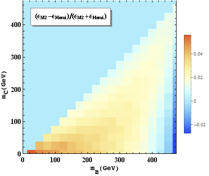
For completeness, in Fig. 12 we also show results for the standard hemisphere method [31, 32, 33, 34] when applied to our event topology. In the hemisphere method, one clusters the visible particles into two groups trying to keep the invariant mass of each cluster to a minimum. It is not difficult to see that in our language this is nothing but the method. The corresponding efficiency is shown in the middle panel of Fig. 12 and it exhibits the same qualitative behavior. The right panel of Fig. 12 compares the two methods by plotting the fractional difference of their efficiencies. We see that throughout most of the parameter space, the efficiency of the method is higher by 2-5%.
7 Summary and outlook
The combinatorial problem is a very important issue in experimental particle physics. Identifying the correct event topology on an event by event basis is a key element of many analyses which attempt to measure particle properties such as spin, couplings, CP quantum numbers, etc. A successful method which can avoid combinatorial ambiguities, especially in jetty events, is bound to improve the sensitivity of new physics searches as well.
In this paper, we revisited some of the existing methods [36, 53] for resolving the combinatorial ambiguity in the dilepton event topology of Fig. 1. To summarize our main findings:
- 1.
- 2.
Step II does not lead to any appreciable effect after Step I, and can be safely omitted from the algorithm.
- 3.
The use of the variable in Step III is counterproductive, and can also be dropped from consideration.
- 4.
The use of a single optimal variable at Step III (as opposed to a combination of variables) is generally sufficient to produce the desired result.
- 5.
The efficiency is also increased if the available mass information is incorporated as early as possible, e.g., by utilizing the variables and , as discussed in section 5.2.
- 6.
We investigated further improvements of the algorithm, by invoking other types of variables, including a global inclusive variable like and an angular variable like , see section 5.3.
- 7.
In section 6 we discussed a more general approach which does not rely on any mass information.
One should keep in mind that the efficiency can always be further improved at the cost of statistics. For instance, a cut on reduces the number of signal events, but the resulting efficiency can be increased beyond [53].
Our results are directly applicable to any studies of final states containing . In searches for new physics, dilepton would be the dominant background and our results should help in reducing it and increasing the sensitivity. In addition, there are several interesting physics scenarios where a similar combinatorial problem plagues the signal itself:
Looking ahead, there are several directions in which the study presented here can be evolved.
- 1.
Following the previous literature, in this initial investigation we considered a relatively simple situation, where there were only two possible alternatives, and we had to pick one of them. As we increase the number of indistinguishable objects in the final state, things get much more complicated. We intend to tackle this more difficult problem in the very near future.
- 2.
As the number of jets in the signature is increased, it becomes important to cross-check the parton-level results with more detailed simulations including detector effects, initial and final state radiation, etc.
- 3.
The kinematic variables which we used here were designed for event topologies with 2 missing particles. It would be interesting to generalize our analysis to event topologies with more than 2 missing particles, where one would have to use a different set of variables suitably adapted for that case.
Acknowledgements.
This work is supported in part by a US Department of Energy grant DE-SC0010296 and DE-FG02-12ER41809. DD acknowledges support from the University of Florida Informatics Institute in the form of a Graduate Student Fellowship. DK is supported by the Korean Research Foundation (KRF) through the CERN-Korea Fellowship program. JHK is supported in part by the University of Kansas General Research Fund allocation 2302091.References
- (1) CMS collaboration, S. Chatrchyan et al., Missing transverse energy performance of the CMS detector, JINST 6 (2011) P09001, [1106.5048].
- (2) S. Chang and A. de Gouvea, Neutrino alternatives for missing energy events at colliders, Phys. Rev. D80 (2009) 015008, [0901.4796].
- (3) K. Agashe, D. Kim, M. Toharia and D. G. E. Walker, Distinguishing Dark Matter Stabilization Symmetries Using Multiple Kinematic Edges and Cusps, Phys. Rev. D82 (2010) 015007, [1003.0899].
- (4) K. Agashe, D. Kim, D. G. E. Walker and L. Zhu, Using to Distinguish Dark Matter Stabilization Symmetries, Phys. Rev. D84 (2011) 055020, [1012.4460].
- (5) G. F. Giudice, B. Gripaios and R. Mahbubani, Counting dark matter particles in LHC events, Phys. Rev. D85 (2012) 075019, [1108.1800].
- (6) W. S. Cho, D. Kim, K. T. Matchev and M. Park, Probing Resonance Decays to Two Visible and Multiple Invisible Particles, Phys. Rev. Lett. 112 (2014) 211801, [1206.1546].
- (7) K. Agashe, R. Franceschini, D. Kim and K. Wardlow, Using Energy Peaks to Count Dark Matter Particles in Decays, Phys. Dark Univ. 2 (2013) 72–82, [1212.5230].
- (8) A. J. Barr, T. J. Khoo, P. Konar, K. Kong, C. G. Lester, K. T. Matchev et al., Guide to transverse projections and mass-constraining variables, Phys. Rev. D84 (2011) 095031, [1105.2977].
- (9) T. Plehn, D. Rainwater and P. Z. Skands, Squark and gluino production with jets, Phys. Lett. B645 (2007) 217–221, [hep-ph/0510144].
- (10) J. Alwall, S. de Visscher and F. Maltoni, QCD radiation in the production of heavy colored particles at the LHC, JHEP 02 (2009) 017, [0810.5350].
- (11) A. Papaefstathiou and B. Webber, Effects of QCD radiation on inclusive variables for determining the scale of new physics at hadron colliders, JHEP 06 (2009) 069, [0903.2013].
- (12) P. Jackson, C. Rogan and M. Santoni, Sparticles in motion: Analyzing compressed SUSY scenarios with a new method of event reconstruction, Phys. Rev. D95 (2017) 035031, [1607.08307].
- (13) A. J. Barr and C. G. Lester, A Review of the Mass Measurement Techniques proposed for the Large Hadron Collider, J. Phys. G37 (2010) 123001, [1004.2732].
- (14) I. Hinchliffe, F. E. Paige, M. D. Shapiro, J. Soderqvist and W. Yao, Precision SUSY measurements at CERN LHC, Phys. Rev. D55 (1997) 5520–5540, [hep-ph/9610544].
- (15) D. R. Tovey, Measuring the SUSY mass scale at the LHC, Phys. Lett. B498 (2001) 1–10, [hep-ph/0006276].
- (16) P. Konar, K. Kong and K. T. Matchev, : A Global inclusive variable for determining the mass scale of new physics in events with missing energy at hadron colliders, JHEP 03 (2009) 085, [0812.1042].
- (17) J. Hubisz, J. Lykken, M. Pierini and M. Spiropulu, Missing energy look-alikes with 100 pb-1 at the LHC, Phys. Rev. D78 (2008) 075008, [0805.2398].
- (18) C. G. Lester and D. J. Summers, Measuring masses of semiinvisibly decaying particles pair produced at hadron colliders, Phys. Lett. B463 (1999) 99–103, [hep-ph/9906349].
- (19) B. C. Allanach, C. G. Lester, M. A. Parker and B. R. Webber, Measuring sparticle masses in nonuniversal string inspired models at the LHC, JHEP 09 (2000) 004, [hep-ph/0007009].
- (20) C. Lester and A. Barr, MTGEN: Mass scale measurements in pair-production at colliders, JHEP 12 (2007) 102, [0708.1028].
- (21) J. Alwall, K. Hiramatsu, M. M. Nojiri and Y. Shimizu, Novel reconstruction technique for New Physics processes with initial state radiation, Phys. Rev. Lett. 103 (2009) 151802, [0905.1201].
- (22) Y. Bai and H.-C. Cheng, Identifying Dark Matter Event Topologies at the LHC, JHEP 06 (2011) 021, [1012.1863].
- (23) D. Wiesler, Combinatorial and off-shell effects in new physics cascades. PhD thesis, Hamburg U., 2012.
- (24) P. S. B. Dev, D. Kim and R. N. Mohapatra, Disambiguating Seesaw Models using Invariant Mass Variables at Hadron Colliders, JHEP 01 (2016) 118, [1510.04328].
- (25) D. Kim, K. T. Matchev and M. Park, Using sorted invariant mass variables to evade combinatorial ambiguities in cascade decays, JHEP 02 (2016) 129, [1512.02222].
- (26) M. D. Klimek, Ordered Kinematic Endpoints for 5-body Cascade Decays, JHEP 12 (2016) 132, [1610.08603].
- (27) D. Debnath, J. S. Gainer, C. Kilic, D. Kim, K. T. Matchev and Y.-P. Yang, Detecting kinematic boundary surfaces in phase space: particle mass measurements in SUSY-like events, 1611.04487.
- (28) J. H. Shim and H. S. Lee, Improving combinatorial ambiguities of events using neural networks, Phys. Rev. D89 (2014) 114023, [1402.3907].
- (29) D. Krohn, L. Randall and L.-T. Wang, On the Feasibility and Utility of ISR Tagging, 1101.0810.
- (30) D. Kim and K. Kong, Kinematic discrimination of tW and productions using initial state radiation, Phys. Lett. B751 (2015) 512–524, [1503.03872].
- (31) CMS collaboration, G. L. Bayatian et al., CMS technical design report, volume II: Physics performance, J. Phys. G34 (2007) 995–1579.
- (32) S. Matsumoto, M. M. Nojiri and D. Nomura, Hunting for the Top Partner in the Littlest Higgs Model with T-parity at the CERN LHC, Phys. Rev. D75 (2007) 055006, [hep-ph/0612249].
- (33) W. S. Cho, K. Choi, Y. G. Kim and C. B. Park, Measuring superparticle masses at hadron collider using the transverse mass kink, JHEP 02 (2008) 035, [0711.4526].
- (34) M. M. Nojiri, Y. Shimizu, S. Okada and K. Kawagoe, Inclusive transverse mass analysis for squark and gluino mass determination, JHEP 06 (2008) 035, [0802.2412].
- (35) A. Rajaraman and F. Yu, A New Method for Resolving Combinatorial Ambiguities at Hadron Colliders, Phys. Lett. B700 (2011) 126–132, [1009.2751].
- (36) P. Baringer, K. Kong, M. McCaskey and D. Noonan, Revisiting Combinatorial Ambiguities at Hadron Colliders with , JHEP 10 (2011) 101, [1109.1563].
- (37) M. M. Nojiri, K. Sakurai, Y. Shimizu and M. Takeuchi, Handling jets + missing E(T) channel using inclusive m(T2), JHEP 10 (2008) 100, [0808.1094].
- (38) P. Jackson and C. Rogan, Recursive Jigsaw Reconstruction: HEP event analysis in the presence of kinematic and combinatoric ambiguities, 1705.10733.
- (39) M. M. Nojiri, G. Polesello and D. R. Tovey, Proposal for a new reconstruction technique for SUSY processes at the LHC, in Physics at TeV colliders. Proceedings, Workshop, Les Houches, France, May 26-June 3, 2003, 2003. hep-ph/0312317.
- (40) K. Kawagoe, M. M. Nojiri and G. Polesello, A New SUSY mass reconstruction method at the CERN LHC, Phys. Rev. D71 (2005) 035008, [hep-ph/0410160].
- (41) H.-C. Cheng, J. F. Gunion, Z. Han, G. Marandella and B. McElrath, Mass determination in SUSY-like events with missing energy, JHEP 12 (2007) 076, [0707.0030].
- (42) H.-C. Cheng, D. Engelhardt, J. F. Gunion, Z. Han and B. McElrath, Accurate Mass Determinations in Decay Chains with Missing Energy, Phys. Rev. Lett. 100 (2008) 252001, [0802.4290].
- (43) H.-C. Cheng, J. F. Gunion, Z. Han and B. McElrath, Accurate Mass Determinations in Decay Chains with Missing Energy. II, Phys. Rev. D80 (2009) 035020, [0905.1344].
- (44) D. Kim, K. T. Matchev, F. Moortgat and L. Pape, Testing Invisible Momentum Ansatze in Missing Energy Events at the LHC, 1703.06887.
- (45) A. Barr, C. Lester and P. Stephens, m(T2): The Truth behind the glamour, J. Phys. G29 (2003) 2343–2363, [hep-ph/0304226].
- (46) M. Burns, K. Kong, K. T. Matchev and M. Park, Using Subsystem MT2 for Complete Mass Determinations in Decay Chains with Missing Energy at Hadron Colliders, JHEP 03 (2009) 143, [0810.5576].
- (47) A. J. Barr, B. Gripaios and C. G. Lester, Transverse masses and kinematic constraints: from the boundary to the crease, JHEP 11 (2009) 096, [0908.3779].
- (48) P. Konar, K. Kong, K. T. Matchev and M. Park, Dark Matter Particle Spectroscopy at the LHC: Generalizing M(T2) to Asymmetric Event Topologies, JHEP 04 (2010) 086, [0911.4126].
- (49) P. Konar, K. Kong, K. T. Matchev and M. Park, Superpartner Mass Measurement Technique using 1D Orthogonal Decompositions of the Cambridge Transverse Mass Variable , Phys. Rev. Lett. 105 (2010) 051802, [0910.3679].
- (50) W. S. Cho, K. Choi, Y. G. Kim and C. B. Park, M(T2)-assisted on-shell reconstruction of missing momenta and its application to spin measurement at the LHC, Phys. Rev. D79 (2009) 031701, [0810.4853].
- (51) C. B. Park, Reconstructing the heavy resonance at hadron colliders, Phys. Rev. D84 (2011) 096001, [1106.6087].
- (52) D. Guadagnoli and C. B. Park, -reconstructed invisible momenta as spin analizers, and an application to top polarization, JHEP 01 (2014) 030, [1308.2226].
- (53) K. Choi, D. Guadagnoli and C. B. Park, Reducing combinatorial uncertainties: A new technique based on MT2 variables, JHEP 11 (2011) 117, [1109.2201].
- (54) R. Mahbubani, K. T. Matchev and M. Park, Re-interpreting the Oxbridge stransverse mass variable MT2 in general cases, JHEP 03 (2013) 134, [1212.1720].
- (55) W. S. Cho, J. S. Gainer, D. Kim, K. T. Matchev, F. Moortgat, L. Pape et al., On-shell constrained variables with applications to mass measurements and topology disambiguation, JHEP 08 (2014) 070, [1401.1449].
- (56) G. G. Ross and M. Serna, Mass determination of new states at hadron colliders, Phys. Lett. B665 (2008) 212–218, [0712.0943].
- (57) CMS collaboration, S. Chatrchyan et al., Measurement of masses in the system by kinematic endpoints in pp collisions at = 7 TeV, Eur. Phys. J. C73 (2013) 2494, [1304.5783].
- (58) ATLAS collaboration, Top quark mass measurement in the channel using the mT2 variable at ATLAS, ATLAS-CONF-2012-082 (2012) .
- (59) T. H. N. Phan, Measurement of the top quark mass in the dilepton decay channel using the and variables with ATLAS data, Master’s thesis, Bonn U., 2013-09-02.
- (60) CMS collaboration, A. M. Sirunyan et al., Measurement of the top quark mass in the dileptonic ttbar decay channel using the mass observables Mbl, MT2, and Mblv in pp collisions at sqrt(s) = 8 TeV, 1704.06142.
- (61) W. S. Cho, J. S. Gainer, D. Kim, K. T. Matchev, F. Moortgat, L. Pape et al., Improving the sensitivity of stop searches with on-shell constrained invariant mass variables, JHEP 05 (2015) 040, [1411.0664].
- (62) J. Reuter and D. Wiesler, Distorted mass edges at LHC from supersymmetric leptoquarks, Phys. Rev. D84 (2011) 015012, [1010.4215].
- (63) K. Choi, S. Choi, J. S. Lee and C. B. Park, Reconstructing the Higgs boson in dileptonic W decays at hadron collider, Phys. Rev. D80 (2009) 073010, [0908.0079].
- (64) W. S. Cho, K. Choi, Y. G. Kim and C. B. Park, Mass and Spin Measurement with M(T2) and MAOS Momentum, Nucl. Phys. Proc. Suppl. 200-202 (2010) 103–112, [0909.4853].
- (65) K. Choi, J. S. Lee and C. B. Park, Measuring the Higgs boson mass with transverse mass variables, Phys. Rev. D82 (2010) 113017, [1008.2690].
- (66) J. Alwall, M. Herquet, F. Maltoni, O. Mattelaer and T. Stelzer, MadGraph 5 : Going Beyond, JHEP 06 (2011) 128, [1106.0522].
- (67) W. S. Cho, J. S. Gainer, D. Kim, S. H. Lim, K. T. Matchev, F. Moortgat et al., OPTIMASS: A Package for the Minimization of Kinematic Mass Functions with Constraints, JHEP 01 (2016) 026, [1508.00589].
- (68) D. R. Tovey, On measuring the masses of pair-produced semi-invisibly decaying particles at hadron colliders, JHEP 04 (2008) 034, [0802.2879].
- (69) K. T. Matchev and M. Park, A General method for determining the masses of semi-invisibly decaying particles at hadron colliders, Phys. Rev. Lett. 107 (2011) 061801, [0910.1584].
- (70) W. S. Cho, J. E. Kim and J.-H. Kim, Amplification of endpoint structure for new particle mass measurement at the LHC, Phys. Rev. D81 (2010) 095010, [0912.2354].
- (71) T. Huang, J. M. No, L. Pernié, M. Ramsey-Musolf, A. Safonov, M. Spannowsky et al., Resonant Di-Higgs Production in the Channel: Probing the Electroweak Phase Transition at the LHC, 1701.04442.
- (72) M. R. Buckley and D. Goncalves, Boosting the Direct CP Measurement of the Higgs-Top Coupling, Phys. Rev. Lett. 116 (2016) 091801, [1507.07926].
- (73) C. Englert, J. Ferrando and K. Nordström, Constraining new resonant physics with top spin polarisation information, 1703.05613.
- (74) A. Papaefstathiou and K. Sakurai, Triple Higgs boson production at a 100 TeV proton-proton collider, JHEP 02 (2016) 006, [1508.06524].
- (75) C. Englert, Q. Li, M. Spannowsky, M. Wang and L. Wang, VBS production at the HL-LHC and a 100 TeV pp-collider, 1702.01930.
- (76) J. M. Kunkle, Multiboson measurements and limits on Anomalous Gauge Couplings from the CMS Experiment, in Proceedings, Meeting of the APS Division of Particles and Fields (DPF 2015): Ann Arbor, Michigan, USA, 4-8 Aug 2015, 2015. 1511.00143.
- (77) ATLAS collaboration, M. Aaboud et al., Measurement of vector-boson scattering and limits on anomalous quartic gauge couplings with the ATLAS detector, 1611.02428.
- (78) CMS collaboration, V. Khachatryan et al., Study of vector boson scattering and search for new physics in events with two same-sign leptons and two jets, Phys. Rev. Lett. 114 (2015) 051801, [1410.6315].