Study of Electroweak Vacuum Stability from Extended Higgs Portal of Dark Matter and Neutrinos
Purusottam Ghosha,11 1 pghoshiitg@gmail.com, Abhijit Kumar Sahaa,22 2 abhijit.saha@iitg.ernet.in, Arunansu Sila,33 3 asil@iitg.ernet.in
a Department of Physics, Indian Institute of Technology Guwahati, 781039 Assam, India
Abstract
We investigate the electroweak vacuum stability in an extended version of the Standard Model which incorporates two additional singlet scalar fields and three right handed neutrinos. One of these extra scalars plays the role of dark matter while the other scalar not only helps in making the electroweak vacuum stable but also opens up the low mass window of the scalar singlet dark matter ( 500 GeV). We consider the effect of large neutrino Yukawa coupling on the running of Higgs quartic coupling. We have analyzed the constraints on the model and identify the range of parameter space which is consistent with neutrino mass, appropriate relic density and direct search limits from the latest XENON 1T preliminary result as well as realizing the stability of the electroweak vacuum upto the Planck scale.
1 Introduction
The discovery of the Higgs boson[1, 2, 3] has been considered as the greatest triumph in present day particle physics. Although the experimental search is still on in order to investigate the Higgs boson’s properties, several theoretical and phenomenological reasons are there to push us toward hunting for an enlarged Higgs sector compared to the one present in Standard model (SM). For example the Higgs quartic coupling in SM becomes negative at a high energy scale ( GeV) leading to a possible instability of Higgs vacuum. The present measured values of Higgs mass GeV[4] and top mass GeV[4], suggest that the electroweak (EW) vacuum can be metastable [5, 6, 7, 8, 9, 10, 11]. However the conclusion exclusively depends on the precise measurement of the top mass[12, 13]. Also the metastability of the Universe is not a very robust situation in the context of cosmological inflation[14]. One of the possible solutions to this is to introduce new physics between EW scale and . In view of SM’s incompetence in resolving some of the other issues like dark matter, neutrino mass, matter antimatter symmetry, inflation etc, the introduction of new physics is of course a welcome feature.
In particular, SM fails to accommodate a significant share in terms of its content called dark matter(DM). The most economical and popular scenario is the singlet scalar extension of the SM[15, 16, 17, 18, 19, 20, 21, 22, 23] having Higgs portal interaction. The stability of the dark matter is ensured by imposing a symmetry on it. The relic abundance and corresponding direct detection cross section are solely determined by the DM (the scalar singlet) mass and its coupling with Higgs ( portal coupling). However present experiments, LUX[24] and XENON1T[25], strongly disfavor the model below GeV except the resonance region. The bound on Higgs invisible decay width further constrain the model for GeV[26]. Hence a large range of DM mass seems to be excluded within this simplest framework which otherwise would be an interesting region of search for several ongoing and future direct[24, 25, 27] and indirect experiments[28]. It is interesting to note that the presence of extra scalar in the form of DM can shift the instability scale () toward larger value compared to the SM one ()[29, 30, 31, 32, 33, 34, 35].
On the other hand to accommodate non-zero neutrino mass via type-I seesaw mechanism, one can extend SM with three right handed(RH) neutrinos. The RH neutrinos, being SM singlet, will have standard Yukawa like coupling involving Higgs and lepton doublets. The presence of the neutrino Yukawa coupling affects the running of the Higgs quartic coupling similar to the top Yukawa coupling. In fact with neutrino Yukawa coupling, , of , could be lower than [36, 38, 39, 40, 41, 42, 43, 44, 45, 46, 47], that might lead to an unstable Universe. The situation does not alter much even if one includes scalar singlet DM ( GeV) in this framework [34, 36, 37, 48, 49, 50]. So the combined framework of RH neutrinos and scalar singlet DM excludes a significant range of DM mass ( GeV) while keeping the EW vacuum on the verge of being unstable.
With an endeavour to make the EW vacuum absolutely stable upto the planck scale , in a scenario that can accommodate both the DM and massive neutrinos with large (in type-I seesaw) and simultaneously to reopen the window for lighter scalar singlet DM mass ( 500 GeV), we incorporate two SM real singlet scalars and three SM singlet RH neutrinos in this work.
Similar models to address DM phenomenology involving additional scalars (without involving RH neutrinos) have been studied [51, 35, 52, 53, 54, 55], however with different motivations. Our set up also differs from them in terms of inclusion of light neutrino mass through type-I seesaw. The proposed model has several important ingredients which are mentioned below along with their importance.
- •
One of the additional SM singlet scalars is our DM candidate whose stability is achieved with an unbroken symmetry.
- •
The other scalar would acquire a nonzero vacuum expectation value (vev). This field has two fold contributions in our analysis: (i) it affects the running of the SM Higgs quartic coupling and (ii) the dark matter phenomenology becomes more involved due to its mixing with the SM Higgs and the DM.
- •
The set up also contains three RH neutrinos in order to generate non-zero light neutrino mass through type-I seesaw mechanism. Therefore, along with the contributions from the additional scalar fields, neutrino Yukawa coupling, , is also involved in studying the running of the Higgs quartic coupling.
We observe that the presence of the scalar44 4 This scalar perhaps can be identified with moduli/inflaton fields [61, 60, 59, 58, 57] or messenger field[62] connecting SM and any hidden sector. with non-zero vev affects the DM phenomenology in such a way that less than 500 GeV becomes perfectly allowed mass range considering the recent XENON-1T result[25], which otherwise was excluded from the DM direct search results[56]. We also include XENON-nT[25] prediction to further constrain our model. On the other hand, we find that the SM Higgs quartic coupling may remain positive till (or upto some other scale higher than ) even in presence of large , thanks to the involvement of the scalar with non-zero vev. We therefore identify the relevant parameter space (in terms of stability, metastability and instability regions) of the model which can allow large (with different mass scales of RH neutrinos) and scalar DM below 500 GeV. Bounds from other related aspects, lepton flavor violating decays, neutrinoless double beta decay etc., are also considered. The set-up therefore demands rich phenomenology what we present in the following sections.
The paper is organized as follows. In section 2, we discuss the set-up of our model and in section 3, we include the constraints on our model parameters. Then in the subsequent sections 4 and 5, we discuss the DM phenomenology and vacuum stability respectively in the context of our model. In section 6, we discuss connection of the model with other observables. Finally we conclude in section 7.
2 The Model
As mentioned in the introduction, we aim to study how the EW vacuum can be made stable in a model that would successfully accommodate a scalar DM and neutrino mass. For this purpose, we extend the SM by introducing two SM singlet scalar fields, and , and three right-handed neutrinos, . We have also imposed a discrete symmetry, . The field is odd (even) under () and is even (odd) under () while all other fields are even under both and . There exists a non-zero vev associated with the field. The unbroken ensures the stability of our dark matter candidate . On the other hand, the inclusion of simplifies the scalar potential in the set-up55 5 A spontaneous breaking of discrete symmetry may lead to cosmological domain wall problem [63]. To circumvent it, one may introduce explicit breaking term in higher order which does not affect our analysis.. The RH neutrinos are included in order to incorporate the light neutrino mass through type-I seesaw mechanism.
The scalar potential involving and the SM Higgs doublet () is given by
| (1) |
where
The relevant part of the Lagrangian responsible for neutrino mass is given by
where are the left-handed lepton doublets, is the Majorona mass matrix of the RH neutrinos. This leads to the light neutrino mass, with GeV as the vacuum expectation value of the SM Higgs. Minimization of the potential leads to the following vevs of and (the neutral component of ), as given by66 6 Note that due to the absence of any breaking term in the Lagrangian of our model, panic vacua [64, 65, 55] do not appear here.
| (2) | |||
| (3) |
So after gets the vev and electroweak symmetry is broken, the mixing between and will take place and new mass or physical eigenstates, and , will be formed. The two physical eigenstates are related with and by
| (4) |
where the mixing angle is defined by
| (5) |
Similarly the mass eigenvalues of these physical Higgses are found to be
| (6) | |||
| (7) |
Using Eqs.(5,6,7), the couplings , and can be expressed in terms of the masses of the physical eigenstates and , the vevs (, ) and the mixing angle as
| (8) | ||||
| (9) | ||||
| (10) |
Among and , one of them would be the Higgs discovered at LHC. The other Higgs can be heavier or lighter than the SM Higgs. Below we proceed to discuss the constraints to be imposed on the couplings and mass parameters of the model before studying the DM phenomenology and vacuum stability in the subsequent sections.
3 Constraints
Here we put together the constraints (both theoretical and experimental) that we will take into account to find the parameter space of our model.
- •
- •
In addition, the perturbative unitarity associated with the matrix corresponding to 2 2 scattering processes involving all two particles initial and final states [68, 69] are considered. In the specific model under study, there are eleven neutral and four singly charged combinations of two-particle initial/final states. The details are provided in Appendix A. It turns out that the some of the scalar couplings of Eq.(1) are bounded by
(12) The other scalar couplings are restricted (in form of combinations among them) from the condition that the roots of a polynomial equation should be less than 16 (see Eq.(A.22) of Appendix A).
- •
To maintain the perturbativity of all the couplings, we impose the condition that the scalar couplings should remain below 4 while Yukawa couplings are less than till . An upper bound on follows from the perturbativity of [70] with a specific choice of .
- •
Turning into the constraints obtained from experiments, we note that the observed signal strength of the 125 GeV Higgs boson at LHC [73, 74, 75, 76, 77, 71] provides a limit on as, with GeV. The analysis in [72] shows that is restricted significantly () by the direct Higgs searches at colliders [73, 74, 75, 76, 77] and combined Higgs signal strength [78] for 150 GeV GeV while for 300 GeV 800 GeV, it is the NLO contribution to the boson mass [70] which restricts in a more stipulated range. Corrections to the electroweak precision observables through the parameters turn out to be less dominant compared to the limits obtained from boson mass correction [70]. For our purpose, we consider for the analysis.
Apart from these, we impose the constraints on from lepton flavor violating decays. Also phenomenological limits obtained on the scalar couplings involved in order to satisfy the relic density [79] and direct search limits[25] by our dark matter candidate are considered when stability of the EW minimum is investigated.
4 Dark matter phenomenology
The scalar field playing the role of dark matter has a mass given by as followed from Eq.(1). Before moving toward the relic density calculation in our model, we would like to comment on the simplest odd scalar dark matter scenario in view of recent XENON 1T[25] result. Note that for the purpose of DM phenomenology in this case, the only relevant parameters are given by and the Higgs portal coupling (or and ).
  |
In Fig.1 (left panel), we provide a contour plot for relic density consistent with the Planck result[79] in the plane indicated by the blue solid line. In the right panel of Fig.1, we provide the DM-nucleon cross section evaluated with the value of corresponding to the value as obtained from the left panel plot. We then incorporate the direct search limits on the DM-nucleon cross section as obtained from LUX 2016 [24], and the most recent XENON 1T[25] result [25] in the same plot denoted by blue and red dashed lines respectively. We conclude that the dark matter mass below 500 GeV is excluded from the present XENON 1T[25] result. This result is indicated by the red portion of the contour line in the left panel, while the remaining blue portion of the contour plot ( of the left panel) represents the allowed range of satisfying both the relic density and direct search constraints.
Let us now move to the relic density estimate in our set-up with the extra scalar and compare the phenomenology with the simplest scalar DM scenario in the light of the mixing between the SM Higgs and . Using Eq.(4) and inserting them into the SM Lagrangian along with the ones mentioned in Eq.(1), we obtain the following list of interaction vertices involving two Higgses ( and ), dark matter field () and several other SM fields.
Following Eq.(4) we draw the Feynman diagrams for DM annihilation channels into SM particles and to the second Higgs in Fig.2.
It is expected that the DM candidate is in thermal equilibrium with the SM degrees of freedom in the early universe. We therefore proceed to evaluate their abundance through the standard freeze-out mechanism. The Boltzmann equation,
| (14) |
is employed for this purpose, where is the number density of the dark matter , H is the Hubble parameter, represents the total annihilation cross-section as given by . We consider here the RH neutrinos to be massive enough compared to the DM mass. So RH neutrinos do not participate in DM phenomenology. We have then used the MicrOmega package[80] to evaluate the final relic abundance of DM.
We have the following parameters in our set-up,
| (15) |
The parameters is involved in the definition of . Parameters can be written in terms of other parameters as shown in Eqs.(8,9,10). Among all the parameters in Eq.(15), does not play any significant role in DM analysis.
We first assume as the Higgs discovered at LHC i.e. 125.09 GeV[4] and the other Higgs is the heavier one (). It would be appealing in view of LHC accessibility to keep below 1 TeV. In this case limits on are applicable as discussed in Section 3 depending on specific value of [72]. Now in this regime (where is not too heavy, in particular TeV), is bounded by [72] and we have taken here a conservative choice by fixing . Note that in the small approximation, is mostly dominated by the SM Higgs doublet . In this limit the second term in Eq.(8) effectively provides the threshold correction to [82, 57, 81] which helps in achieving vacuum stability as we will see later. Furthermore considering this threshold effect to be equal or less than the first term in Eq.(8) (i.e. approximately the SM value of ), we obtain an upper bound on as . Therefore in case with , our working regime of can be considered within . We take to be 300 GeV for our analysis.
Note that with small , almost coincides with the second term in Eq.(9). It is quite natural to keep the magnitude of a coupling below unity to maintain the perturbativity limit for all energy scales including its running. Hence with the demand , one finds . To show it numerically, let us choose , then we obtain GeV. Therefore with GeV, a lower limit on GeV can be set. We consider to be 800 GeV so that turns out to be 0.307.
On the other hand, if we consider the other Higgs to be lighter than the one discovered at LHC, we identify to be the one found at LHC and hence GeV. Then Eq.(4) suggests as the complete decoupling limit of the second Higgs. Following the analysis in [83, 72, 84, 85, 86, 87], we infer that most of the parameter space except for a very narrow region both in terms of mixing angle () and mass of the lighter Higgs () GeV, is excluded from LEP and LHC searches.

Such a range is not suitable for our purpose as can bee seen from Eq.(8). In this large limit, gets the dominant contribution from the second term in Eq.(8) where the first term serves the purpose of threshold effect on . However being smaller than (the SM like Higgs), this effect would not be sufficient to enhance such that its positivity till can be ensured. Therefore we discard the scenario (SM like Higgs) from our discussion. Hence the DM phenomenology basically depends on and .
In a direct detection experiment, the DM scatters with the nucleon through the exchange of and as shown schematically in Fig.3 . The resulting spin-independent cross-section of DM-nucleon elastic scattering is given by [35] :
| (16) |
where [88, 89]. The couplings appeared as are specified in the list of vertices in Eq.(4). Below we discuss how we can estimate the relevant parameters (, and ) from relic density and direct search limits. For this purpose, we consider GeV and GeV as reference values, unless otherwise mentioned.
4.1 DM mass in region R1: [ GeV]
In this region any decay mode of and into DM is kinematically forbidden following our consideration for GeV. As stated before, we consider to be the SM like Higgs discovered at LHC, with GeV and is fixed at 0.307. Therefore in order to satisfy the relic density [79], we first scan over and for different ranges of dark matter mass where is kept fixed at 0.2. The allowed range of parameter space contributing to the relic abundance satisfying the correct relic density is indicated on plane in Fig.4 (in the top left panel), where different coloured patches indicate different ranges of . In the upper-right plot of Fig.4, the corresponding direct search cross sections for the relic density satisfied points obtained from the upper left plot (including the variation of ) are provided. It can be clearly seen that many of these points lie below the LUX 2016[24] experimental limit for a wide range of dark matter mass (indicated by the colors depicted in the inset of Fig.4, upper left panel).


From the top left panel of Fig.4, the relic density contour plot (with a particular ) in - plane shows that there exists a range of for which the plot is (almost) insensitive to the change in . This becomes more prominent for plots associated with higher dark matter mass. In particular, the contour line satisfying the correct relic density with GeV depicts a sharp variation in (below 0.4) with almost no variation of around 0.13. We now discuss the reason behind such a behaviour. We note that for , the total annihilation cross section satisfying the relic density is mostly dominated by the SM, SM process, specifically dominate. In our scenario, processes are mediated by both the Higgses, and . Although is involved in the vertices characterizing these processes, it turns out that once both the contributions are taken into account, the dependence is effectively canceled leaving the annihilation almost independent of . Hence SM, SM depends mostly on . The other processes like are subdominant (these are allowed provided GeV) in this region with large . Then the total cross section and hence the relic density contour line becomes insensitive to the change in as long as it remains below 0.4 while . This is evident in the top left panel of Fig.4. Similar effects are seen in case of lower ( GeV) as well.
Once we keep on decreasing below 0.13, it turns out that SM, SM becomes less important compared to the (in particular the channel) with beyond 0.4 (in case of GeV). Note that the plot shows the insensitiveness related to in this low region for obvious reason. Similar results follow with GeV also, where provides the dominant contribution in . Based on our discussion so far we note that for the channels with Higgses in the final states contribute more to total . On the other hand for low values of (although comparable to ), the model resembles the usual Higgs portal dark matter scenario where W bosons in the final state dominate. To summarize,
- •
GeV: For low , dominates. However for large , becomes the main annihilation channel.
- •
GeV: New annihilation process opens up. This with contribute dominantly for large . Otherwise the channels with SM particles in final states dominate.
- •
GeV: The annihilation channel opens up in addition to and in the final states. Their relative contributions to total again depend on the value of .
In the top left panel of Fig.4, we also note the existence of a small overlapped region when for the dark matter mass regions between 280-300 GeV and 300-310 GeV. This has been further clarified in Fig.5, where we note that relic density contour lines with GeV and GeV intersect each other around and . Note that when DM mass GeV, in addition to the and annihilation processes, opens up and contribute to the total annihilation cross section ( this new channel can be realized through both and mediation).
Then total annihilation cross section will be enhanced for GeV case, i.e becomes large compared to the GeV mass range where is not present. This enhancement has to be nullified in order to realize the correct relic density and this is achieved by reducing compared to its required value for a fixed and in region. Note that in view of our previous discussion, we already understand that becomes important compared to SM, SM process in the region with . Hence the two mass regions (below and above 300 GeV) overlap in plane as seen in the top left panel of Fig.4 as well in Fig.5. The total annihilation cross section of DM depends on its mass also. However the small mass differences between the two overlapped regions have very mild effect on . Similar effect should be observed below and above 212.5 GeV as opens up there. However we find that around the GeV, even with , the contribution from this particular channel to is negligible as compared to SM SM contribution and hence we do not observe any such overlapped region there.
In the top right panel of Fig.4 we provide the spin-independent (SI) direct detection (DD) cross sections corresponding to the points in the left panel satisfying relic density data having different range of dark matter masses as indicated by the colored patches. We further put the LUX 2016[24], XENON 1T[25] and nT (expected) lines on it. As known, for a lowerer cross section, it reaches the neutrino floor where signals from DM can not be distinguished from that of neutrino. We find that the scenario works with reasonable values of the parameters, i.e. not with any un-naturally small or large values of couplings. Note that once we use the XENON 1T[25] and projected XENON nT[27] limits on the scattering cross section, we would obtain more restricted region of parameter space for as shown in left (with XENON 1T[25]) and right (with XENON nT[27]) figures of the bottom panel. From the plot with XENON-nT prediction, we find that the scenario works even with reasonably large values of required for satisfying the relic density, although they are comparable to each other. This is because of the fact that to keep the direct detection cross section relatively small (even smaller than the XENON nT), it requires a cancellation between and as can be seen from Eq.(16) in conjugation with definition of and for a specific value. Such a cancellation is not that important for plots with LUX 2016[24] or XENON 1T[25] results and hence showing a wider region of parameter space for and .

It can be concluded from upper panel of Fig.4 that the presence of additional singlet scalar field helps in reducing the magnitude of that was required (say ) to produce correct relic density in minimal form of singlet scalar DM or in other words it dilutes the pressure on to produce correct relic density and to satisfy DD cross section simultaneously. For illustrative purpose, let us choose a dark matter mass with 500 GeV. From Fig.1, we found that in order to satisfy the relic density, we need to have a 0.15 which can even be 0.02 in case with large . Similarly we notice that for GeV, was 0.086 in order to produce correct relic density which however was excluded from direct search point of view. This conclusion changes in presence of as we can see from Fig.4, (left panel) that GeV can produce correct relic density and evade the direct search limit with smaller . This is possible in presence of nonzero and small ( here) which redistribute the previously obtained value of into and while simultaneously brings the direct search cross section less than the experimental limit due to its association with (see the definition of and ).


In Fig.7 (left panel), we show the relic density versus plot with our chosen set of parameters, , GeV, , while varying and within and . Similarly in right panel, we provide the relic density vs plot for a different range of and . We note that there are two resonance regions, one at for SM like Higgs and other at with heavy Higgs77 7 As expected, it would be always possible to satisfy the relic density and DD limits within this region. mass at 300 GeV. In left panel for DM heavier than 150 GeV, we find GeV can correctly produce the relic density in the observed range and simultaneously evade the DD limit set by LUX 2016[24]. This result is consistent with the plot in Fig.4. Similarly GeV is in the acceptable range, which is in line with observation in Fig.4. In the left panel of Fig.7 we also have another region of DM mass GeV having correct relic abundance however discarded by LUX 2016. The region was not incorporated in top left panel of Fig.4 as we have started with bigger than 150 GeV only. The possibility of having dark matter lighter than 150 GeV in the present scenario will be discussed in the next subsection. Since in obtaining the Fig.4, we have fixed and , below in Fig.6 and 8, we provide the expected range of two couplings and when are varied for dark matter mass GeV . We find the variation is little sensitive with the change of both and . As or increases for GeV, it requires less for a particular to satisfy the relic density. We have also applied the LUX 2016[24] DD cross section limit in those plots and are indicated by solid black patches. In Fig.8, one dark blue dot has been put on the contour which will be used in study of Higgs vacuum stability as a reference point.


4.2 DM mass in region R2: ( GeV)
Here we briefly discuss the DM phenomenology in the low mass region GeV. In this region, the decay process of heavy higgs to DM () will be active. For further low , both and decay modes will be present.
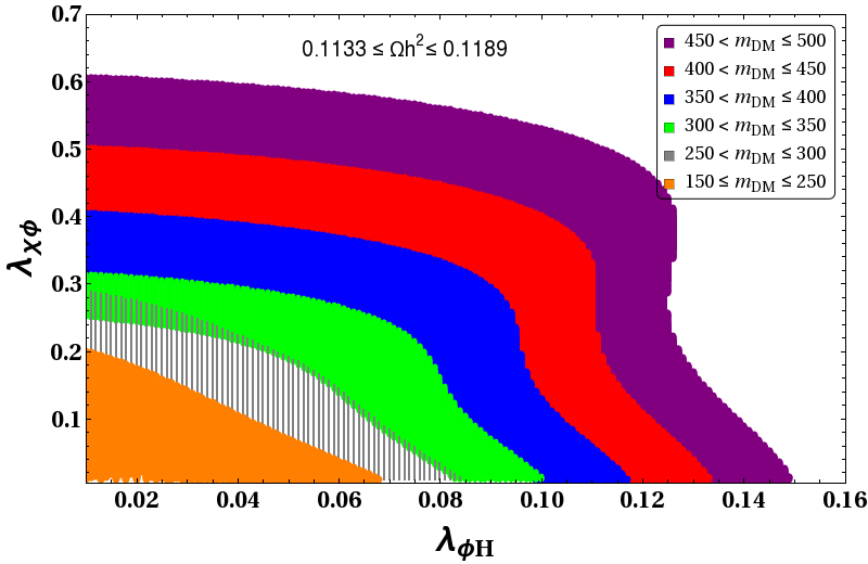
We perform a scan over the region to find the correct relic density satisfied parameter space with allowed direct detection cross section from LUX 2016[24] and XENON 1T experiments[25]. The results are shown in Fig.9, left and right panels where DD limits from LUX 2016 [left panel] and XENON 1T (preliminary) [right panel] are considered separately. In doing these plots, we have considered different mass ranges as indicated by different colors. The color codes are depicted within the inset of each figures. We note that the required , values are almost in the similar range as obtained in Fig.4. We also note that there exists a resonance region through near GeV, indicated by the blue patch. In this resonance region, the relic density becomes insensitive to the coupling and hence the blue patch is extended over the entire region of , in the Fig.9.
Finally we attempt to estimate the required to provide the correct amount of modification over the minimal version of a real singlet DM having interaction with SM Higgs only in order to revive the ‘below 500 GeV’ DM into picture. In other words, the amount of should be enough to satisfy correct relic abundance and DD cross section limits of LUX 2016[24] and XENON 1T[25] for this particular mass range. To do the analysis, we fix while three different values of at 0.04, 0.08 and 0.10 are considered for the study. We then provide the versus plot in Fig.10 which is consistent with relic density and LUX 2016 limits. We infer that a sizable value of is required for this. With , we have noted earlier from Fig. 1 that it alone reproduces the desired relic density with a 330 GeV dark matter, although excluded by LUX 2016 limits. Now we observe from Fig. 10 that in order to make this as a viable DM mass, we need to have a (0.1) with . Such a moderate value of is compatible with LEP and LHC results. A larger value of (0.3) with can accommodate DM mass around 440 GeV as seen from the Fig. 10. Similarly, we indicate that with (for which DM mass GeV and GeV satisfy the relic density as seen from Fig. 1), variation covers a range of DM mass 330-370 GeV [240-290 GeV] provided we restrict ourselves upto .
5 Vacuum stability
In this section, we will discuss how the EW vacuum stability can be achieved in our model. For clarification purpose and a comparative study of it, we first discuss how the presence of different ingredients (three RH neutrinos, DM and extra scalar ) can affect the running of the Higgs quartic coupling when added one after other. We first comment on the inclusion of the RH neutrinos and investigate the running of . Then we study how the involvement of the scalar singlet DM field can alter the conclusion. Finally we discuss the result corresponding to our set-up, including the field as well.
In doing this analysis, the absolute stability of the Higgs vacuum is ensured by for any energy scale where the EW minimum of the scalar potential is the global minimum. However there may exist another minimum which is deeper than the EW one. In that case we need to calculate the tunneling probability of the EW vacuum to the second minimum. The Universe will be in metastable state provided the decay time of EW vacuum is longer than the age of the universe. The tunneling probability is given by[5, 6],
| (17) |
where is the age of the universe. is the scale at which probability is maximized, determined from . Hence for metastable Universe requires[5]
| (18) |
where yr is used. As noted in [6], for , one can safely consider ).
Before proceeding further, some discussion on the involvement of light neutrino mass in the context of vacuum stbaility is pertinent here. As stated before, the light neutrino mass is generated through type-I seesaw for which three RH neutrinos are included in the set up. We now describe the strategy that we adopt here in order to study their impact on RG evolution. For simplicity, the RH neutrino mass matrix is considered to be diagonal with degenerate entries, i.e. . As we will see, it is which enters in the function of the relevant couplings. In order to extract the information on , we employ the type-I mass formula . Naively one would expect that large Yukawas are possible only with very large RH neutrino masses. For example with GeV, comes out to be 0.3 in order to obtain eV. Contrary to our naive expectation, it can be shown that even with smaller one can achieve large values of once a special flavor structure of is considered[38]. Note that we aim to study the EW vacuum stability in presence of large value of . For this purpose, we use the parametrization by [90] and write as
| (19) |
where is the diagonal light neutrino mass matrix and is the unitary matrix diagonalizing the neutrino mass matrix such that . Here represents a complex orthogonal matrix which can be written as with as real orthogonal and as real antisymmetric matrices respectively. Hence one gets
| (20) |
Note that the real antisymmetric matrix does not appear in the seesaw expression for . Therefore with any suitable choice of , it would actually be possible to have sizeable Yukawas even with light and hence this can affect the RG evolution of significantly. As an example, let us consider magnitude of all the entries of to be equal, say with all diagonal entries as zero. Then with = 1 TeV, can be as large as 1 with [90, 91]. Below we specify the details of Higgs vacuum stability in presence of RH neutrinos only.
5.1 Higgs vacuum stability with right-handed neutrinos
In presence of the RH neutrino Yukawa coupling , the renormalization group (RG) equation of SM couplings will be modified[92].
Below we present the one loop beta functions of Higgs quartic coupling , top quark Yukawa coupling and neutrino Yukawa coupling ,
| (21) | ||||
| (22) | ||||
| (23) |
where and represent the functions of and respectively in SM. The dependence is to be evaluated in accordance with the type-I seesaw expression, .
Also with large (elements of ), it is found [38] that Tr and we will be using this approximated relation in obtaining the running of the couplings through Eqs.(21,22,23). Here we have used the best fit values of neutrino oscillation parameters for normal hierarchy[93, 94]. We have also considered the mass of lightest neutrino to be zero.
Note that just like the top quark Yukawa coupling, the neutrino Dirac Yukawa is having a similar impact on the Higgs quartic coupling, in particular with large . Also the top quark Yukawa would have a contribution dependent on . This has been studied in several works[36, 38, 39, 40, 41, 42, 43, 44, 45, 46]. We summarize here the results with some benchmark values of RH neutrino masses. These will be useful for a comparative study with the results specific to our model. In Fig.11 (left panel), we have plotted running of the Higgs quartic coupling against energy scale till for different choices of and GeV with denoted by red, black and green solid lines respectively. The pink shaded portion represents the instability region given by the inequality [5] . As expected, we find that the Higgs quartic coupling enters into the instability region well before the Planck scale.
| Scale | |||||
|---|---|---|---|---|---|
In the right panel of Fig.11, the effect of choosing different within the present uncertainty is shown for a fixed GeV. The black solid, dashed and dotted lines represent the running with as 173.2 GeV, 177 GeV and 171 GeV respectively. In doing this analysis, we fix the initial values of all SM couplings [6] as given in Table 1 at an energy scale . Here we consider GeV, GeV and . In Fig.12, we have shown a region plot for and with fixed at GeV in terms of stability ( remains positive all the way upto ), metastability and instability of the EW vacuum of the SM. The top quark mass is varied between 168 GeV to 178 GeV. The region in which EW vacuum is stable is indicated by green and the metastable region is indicated by white patches. The instability region is denoted with pink shaded part. It can be noted that the result coincides with the one obtained in [41]. We aim to discuss the change obtained over this diagram in the context of our model.
5.2 Higgs vacuum stability from Higgs Portal DM and RH neutrinos
Here we discuss the vacuum stability scenario in presence of both the scalar DM () and three RH neutrinos (). In that case, effective scalar potential becomes only. Note that the DM phenomenology is essentially unaffected from the inclusion of the heavy RH neutrinos with the assumption . On the other hand combining Eq.(21,22,23), we obtain the corresponding beta functions for the couplings as provided below;
| (24) | ||||
| (25) | ||||
From the additional term , we expect that the involvement of DM would affect the EW vacuum stability in a positive way ( pushing the vacuum more toward the stability) as shown in [29, 30, 31, 32, 33, 34] whereas we noted in the previous subsection that the Yukawa coupling (if sizable) has a negative impact on it.
The interplay between the neutrino Yukawa coupling and Higgs portal coupling with DM is shown in Fig. 13, left and right panels (top and bottom). For the purpose of comparison, we have kept the same set of choices of parameters as in Fig.11, (left and right panels ). For the top panels, we consider mass of the dark matter to be GeV and for the bottom set, GeV is taken. The choice of could in turn fix the coupling from the relic density plot of Fig.1. For example with GeV is 0.075 and for GeV, is given by 0.286 value. It is evident that the presence of Higgs portal coupling only has a mild effect as compared to the impact created by the neutrino Yukawa coupling. Finally in Fig.14 we provide the region plot in Tr[] - plane where the stable and instable regions are indicated by green and pink patches. This plot while compared with Fig.12, indicates that there is no such noticeable improvement except the mild enhancement of the metastable region due to the involvement of singlet scalar (DM) with Higgs portal coupling. With an aim to accommodate both the massive neutrinos and a relatively light dark matter ( 500 GeV), we move on to the next section where the field is included.
5.3 EW vacuum stability in extended Higgs portal DM and RH neutrinos
Turning into the discussion on vacuum stability in our framework of extended Higgs portal having three RH neutrinos, DM and the fields, we first put together the relevant RG equations (for ) as given by,
| (27) | ||||
| (28) | ||||
| (29) | ||||
| (30) |
We note that the couplings and which played important role in DM phenomenology, are involved in the running of couplings as well. From the discussion of the DM section, we have estimated these parameters in a range so as to satisfy the appropriate relic density and be within the direct search limits for a specific choice of other parameters at their reference values: GeV and GeV, (henceforth we describe this set as ). In particular an estimate for are obtained from Fig.4 (for 150 GeV 500 GeV) and from Fig. 9 (for 150 GeV) having different choices of and . The parameter dependence is mostly realized through following Eq.(10), where are fixed from set . This is the most crucial parameter which control both the DM phenomenology and the vacuum stability. We have already seen that it allows the scalar singlet DM to be viable for the low mass window by relaxing from its sole role in case of single scalar singlet DM. On the other hand, a non-zero provides a positive shift (it is effectively the threshold effect in the small limit as seen from Eq. (8)) to the Higgs quartic coupling and hence guides the toward more stability. Hence would be a crucial parameter in this study. Note that the RH neutrinos being relatively heavy as compared to the DM, neutrino Yukawa coupling does not play much role in DM phenomenology.
Assuming the validity of this extended SM (with three RH neutrinos and two singlets, ) upto the Planck scale,
we study the running of the Higgs quartic coupling from EW scale to as shown in Fig.15. In obtaining the running, we have considered GeV, and is considered to be 300 GeV. The values of and are fixed at 0.135 and 0.06 respectively (this particular point is denoted by a blue dot, named , on Fig.8 ). It turns out that any other set of and other than this blue dot from Fig. (while GeV is fixed) would not change our conclusion significantly as long as is considered at 0.2. In order to compare the effect of the extra scalar in the theory, we keep the neutrino parameters Tr[] and at their respective values considered in Figs.11, 13.
In the left panel of Fig.15, the running is performed for three different choices of , specifically at 1 TeV, GeV and GeV while top mass is fixed at 173.2 GeV. A similar plot is exercised in right panel of Fig.15 where three different choices of GeV are considered while is fixed at GeV. Contrary to our previous finding in section (see Fig.11, 13 ), we clearly see here that with GeV and GeV, remains positive upto even in presence of large Tr[] . Hence EW vacuum turns out to be absolutely stable. Although there exists other values of and/or , for which EW vacuum still remains unstable, the scale at which enters into the instable region is getting delayed with a noticeable change from earlier cases (Figs.11, 13). This becomes possible due to the introduction of the field having contribution mostly from the parameter. In order to show its impact on stability, in Fig.16 (left panel), we plot running with different choices of for GeV, GeV and GeV while keeping (same as in Fig.15, left panel, black solid line). It shows that while (black solid line) can not make the EW vacuum absolutely stable till , an increase of value 0.3 can do it (dotted line). Similarly in Fig. 16 (right panel), we consider a lowerer as 1 TeV. We have already noticed that such a low with large pushes EW vacuum toward instability at a much lower scale GeV. In order to make the EW vacuum stable with such an and , one requires as seen from the right panel of Fig.16 (dotted line). However such a large is ruled out from the experimental constraints [72]. For representative purpose, we also include study with other denoted by dashed and solid lines.
We provide Fig.17 where the regions with stability, meta-stability and instability are marked green, white and pink patches in the plane containing Tr[] and . With GeV and GeV, similar plots are shown in Fig.18, left and right panels. Finally in Fig.19, we have shown the RG evolution of all the stability conditions in Eq.(11) from to to check their validity all the way upto . For this purpose, we have considered the initial values of the parameters involved in the following way. For values of and corresponding to GeV and GeV, we have considered the benchmark point values as indicated by a blue dot named in Fig.8 . The value of is then followed from Eq.(9) and is chosen to be at 0.7. Values of Tr[ and GeV are chosen for this purpose from Fig.17 (here the benchmark values are denoted by a black dot ). We conclude that all the stability criteria are fulfilled within the framework. Lastly we comment that instead of picking up the point X from relic density contour with in Fig.8 to study vacuum stability in our model, we could have chosen any other point from that curve. As the stability of Higgs vacuum primarily depends on the value of , our conclusion would not change much. However choice of any point having large could make it reaching Landau pole well before in its RG running through Eq.(30). To avoid that one can reduce the value of or less (earlier it was 0.7) which has no direct connection or impact on DM phenomenology and vacuum stability analysis in the proposed set up. In Fig.20, we have shown the running of all parameters from to involved in perturbative unitarity bound for the benchmark point: GeV, , , GeV, =0.06, , GeV and Tr with GeV. The parameters never exceed the upper limits coming from the unitarity bound. We have also confirmed that any other benchmark points wherever mentioned in our analysis satisfy the perturbativity unitarity limit.
We end this section by comparing the results of vacuum stability in presence of (i) only RH neutrinos, (ii) RH neutrinos + DM and (iii) RH neutrinos + DM + extra scalar with non-zero vev, where in each cases neutrino Yukawa coupling has sizeable contributions. For this purpose, we consider GeV and GeV. From Fig.12, for SM + RH neutrinos, we see that stability can not be achieved. The metastability scenario is still valid in this case upto Tr. Next we add a singlet scalar DM candidate with nonzero Higgs portal coupling to SM with RH neutrinos. Fig.14 (left panel) shows, for GeV, stability of EW vacuum still remains elusive. On the other hand the metastability bound on Tr increases slightly from previous limit to 0.28. So DM with mass 300 GeV has mild impact on study of vacuum stability. Finally we add the extra scalar singlet with non zero vev to the SM with RH neutrinos and scalar DM. We have fixed the heavier Higgs mass GeV and . Now in the combined set up of SM, scalar DM, scalar with non zero vev and RH neutrinos, the situation changes drastically from previous case as seen in Fig.17. For the same top and RH neutrino masses, we can now achieve absolute stability upto Tr and the metastability bound on Tr further improved to 0.41. Overall notable enhancement in the stability and metastability region has been observed in Tr plane compared to the earlier cases. Hence, the numerical comparison clearly shows that the extra scalar having non zero mixing with SM Higgs effectively plays the leading role to get absolute vacuum stability in our model.
6 Connection with other observables
In this section, we first discuss in brief the constraints on the parameters of the model that may arise from lepton flavor violating (LFV) decays. The most stringent limit follows from decay process. The branching ratio of such decay process in our set-up is given by[95, 96, 97]
| (31) |
where is the fine sructure constant, runs from 1 to 3, and
| (32) |
The current experimental limit on LFV branching ratio is[4]
| (33) |

Using this limit, we therefore obtain bounds on corresponding to a fixed value which can be converted to constrain in our set up. In obtaining limits on (for fixed ), first note that remains function of and parameter only (see Eq.(19) with ), once the best fit values of neutrino mixing angles[93, 94] are used to evaluate . Hence LFV limit basically constrains the parameter which in turn is used to obtain . This limit is shown on Fig.21 by the brown solid line, the left side of which is the disallowed region by LFV.
In the same plane of Fig.21 we also include the region of the parameter space allowed by both stability and metastability criteria. The green shaded region denotes the absolute stability of Higgs vacuum while the white region satisfies the metastability condition. We also indicate the instability region by pink patch in the same figure under discussion. For this purpose we have used GeV and GeV, , and (corresponding to the benchmark point indicated by X in Fig.8). The brown shaded region is disfavored by the LFV constraint. Hence from Fig.21 we infer that for low , LFV constraints turn out to be stronger one and for high values, is mostly restricted by the stability issue.
It turns out that the proposed scenario does not provide any significant contribution to neutrinoless double beta decay[98, 99, 100, 101, 102, 103] even for relatively low RH neutrino mass ( GeV). This is in line with the observation made in [40]. Before concluding the section, it is perhaps important to comment on the possibility of explaining the baryon asymmetry of the Universe (BAU). The involvement of RH neutrinos would make the leptogenesis natural candidate to explain BAU from the completion point of view. However with the exactly degenerate RH neutrinos (we consider this for simplicity though), it is not possible. Once a small mass-splitting between two heavy RH neutrinos can be introduced (for example by radiative effect [104, 105, 106]), resonant leptogenesis mechanism [107, 108, 109] can be succesfully implemented[110]. Apart from this, provided one can extend our vacuum stability analysis in presence of non-degenerate RH neutrinos[44] with DM and field, usual thermal leptogenesis can also be employed to explain the BAU of the universe.
7 Conclusions
We have considered an extension of the SM by three RH neutrinos and two scalar singlets with an aim to study the EW vacuum stability in a framework that can incorporate a stable light DM within the reach of collider experiments and to explain the light neutrino mass. A symmetry is imposed of which is broken from the vev of one of the scalars. It is known that with a real scalar singlet DM model, present experimental limits by LUX 2016 and XENON 1T rule out DM mass below GeV. Also its presence does not modify the fate of EW vacuum much and hence keep it metastable only. Although metastability is acceptable, it however leaves some unwanted questions if we include primordial inflation in the picture. So an absolute stability of the EW vacuum is more favourable. On the other hand, introduction of RH neutrinos would have large impact on the running of the Higgs quartic coupling due to the neutrino Yukawa interaction. Provided the neutrino Yukawa coupling is as large as (1) or more, it can actually destabilize the EW vacuum. Hence we have tried here achieving the stability of the EW vacuum in presence of RH neutrinos and DM. We also plan to find the possibility of a light scalar DM below 500 GeV. For this purpose, we have introduced additional scalar field which gets a vev. The other scalar among the two introduced does not get a vev and thereby is a good candidate for being a dark matter. The presence of the singlet with non-zero vev helps achieving the vacuum stability through a threshold like correction to . So in this particular scenario i.e. SM extended by DM, three RH neutrinos plus one extra scalar, we have studied the Higgs vacuum stability issue considering large Yukawa coupling and variation of within range of uncertainty. We have found the stability region in the Tr plane has been significantly increased in presence of . Simultaneously mixing of this extra scalar with SM Higgs doublet ensures its involvement in the DM annihilations. This mixing is effectively controlled by the Higgs portal coupling of the scalar which also enters into the running of the Higgs quartic coupling. Hence an interplay between the two conditions: one is to achieve the EW vacuum stability and the other is to find a viable DM below 500 GeV, can actually constrain the parameters involved to some extent. Since the set-up involves several new particles, finding their existence in future and ongoing experiments would be an interesting possibility to search for. Here we have assumed the physical Higgs other than the SM one is heavier. The other situation where the second physical Higgs is lighter than the Higgs discovered at 125 GeV. However this case is not of very interest in the present study as following from Eq.(8), it can be seen that the effective Higgs quartic coupling becomes less than the SM one in this case and this would not help making EW vacuum stable. Also the allowed region for is almost excluded from the decay of . Hence we discard this possibility. One interesting extension of our work could be the study of a SM gauge extension where the involvement of gauges bosons can modify our result. We keep it for a future study.
Appendix
Appendix A Unitarity Constraints
In this section we draw the perturbative unitarity limits on quartic couplings present in our model. Scattering amplitude for any process can be expressed in terms of Legendre polynomial as[68, 69]
where, is the scattering angle and is the Legendre polynomial of order . In high energy limit only s wave () partial amplitude will determine the leading energy dependence of the scattering processes[68, 69]. The unitarity constraint says
| (A.1) |
This constraint Eq.(A.1) can be further translated to a bound on the scattering amplitude [68, 69].
| (A.2) |
In our proposed model we have multiple possible scattering processes. Therefore we need to construct a matrix () considering all possible two particle states. Finally we need to calculate the eigenvalues of and employ the bound as in Eq.(A.2).
In the high energy limit we express the SM Higgs doublet as . Then the scalar potential () in Eq.(1) gives rise to eleven neutral combination of two particle states
| (A.3) |
and four singly charged two particle states
| (A.4) |
Hence we can write the scattering amplitude matrix () in block diagonal form by decomposing it into neutral and singly charged sector as
The submatrices are provided below :
References
- [1] G. Aad et al. [ATLAS Collaboration], Phys. Lett. B 716, 1 (2012) doi:10.1016/j.physletb.2012.08.020 [arXiv:1207.7214 [hep-ex]].
- [2] S. Chatrchyan et al. [CMS Collaboration], Phys. Lett. B 716, 30 (2012) doi:10.1016/j.physletb.2012.08.021 [arXiv:1207.7235 [hep-ex]].
- [3] P. P. Giardino, K. Kannike, I. Masina, M. Raidal and A. Strumia, JHEP 1405, 046 (2014) doi:10.1007/JHEP05(2014)046 [arXiv:1303.3570 [hep-ph]].
- [4] K. A. Olive et al. [Particle Data Group], Chin. Phys. C 38, 090001 (2014). doi:10.1088/1674-1137/38/9/090001
- [5] G. Isidori, G. Ridolfi and A. Strumia, Nucl. Phys. B 609, 387 (2001) doi:10.1016/S0550-3213(01)00302-9 [hep-ph/0104016].
- [6] D. Buttazzo, G. Degrassi, P. P. Giardino, G. F. Giudice, F. Sala, A. Salvio and A. Strumia, JHEP 1312, 089 (2013) doi:10.1007/JHEP12(2013)089 [arXiv:1307.3536 [hep-ph]].
- [7] L. A. Anchordoqui, I. Antoniadis, H. Goldberg, X. Huang, D. Lust, T. R. Taylor and B. Vlcek, JHEP 1302, 074 (2013) doi:10.1007/JHEP02(2013)074 [arXiv:1208.2821 [hep-ph]].
- [8] Y. Tang, Mod. Phys. Lett. A 28, 1330002 (2013) doi:10.1142/S0217732313300024 [arXiv:1301.5812 [hep-ph]].
- [9] G. Degrassi, S. Di Vita, J. Elias-Miro, J. R. Espinosa, G. F. Giudice, G. Isidori and A. Strumia, JHEP 1208, 098 (2012) doi:10.1007/JHEP08(2012)098 [arXiv:1205.6497 [hep-ph]].
- [10] J. Ellis, J. R. Espinosa, G. F. Giudice, A. Hoecker and A. Riotto, Phys. Lett. B 679, 369 (2009) doi:10.1016/j.physletb.2009.07.054 [arXiv:0906.0954 [hep-ph]].
- [11] J. Elias-Miro, J. R. Espinosa, G. F. Giudice, G. Isidori, A. Riotto and A. Strumia, Phys. Lett. B 709, 222 (2012) doi:10.1016/j.physletb.2012.02.013 [arXiv:1112.3022 [hep-ph]].
- [12] V. Branchina, E. Messina and A. Platania, JHEP 1409, 182 (2014) doi:10.1007/JHEP09(2014)182 [arXiv:1407.4112 [hep-ph]].
- [13] G. Degrassi, Nuovo Cim. C 037, no. 02, 47 (2014) doi:10.1393/ncc/i2014-11735-1 [arXiv:1405.6852 [hep-ph]].
- [14] A. Kobakhidze and A. Spencer-Smith, Phys. Lett. B 722, 130 (2013) doi:10.1016/j.physletb.2013.04.013 [arXiv:1301.2846 [hep-ph]].
- [15] V. Silveira and A. Zee, Phys. Lett. 161B, 136 (1985). doi:10.1016/0370-2693(85)90624-0
- [16] J. McDonald, Phys. Rev. D 50, 3637 (1994) doi:10.1103/PhysRevD.50.3637 [hep-ph/0702143 [HEP-PH]].
- [17] J. M. Cline, K. Kainulainen, P. Scott and C. Weniger, Phys. Rev. D 88, 055025 (2013) Erratum: [Phys. Rev. D 92, no. 3, 039906 (2015)] doi:10.1103/PhysRevD.92.039906, 10.1103/PhysRevD.88.055025 [arXiv:1306.4710 [hep-ph]].
- [18] W. L. Guo and Y. L. Wu, JHEP 1010, 083 (2010) doi:10.1007/JHEP10(2010)083 [arXiv:1006.2518 [hep-ph]].
- [19] F. S. Queiroz and K. Sinha, Phys. Lett. B 735, 69 (2014) doi:10.1016/j.physletb.2014.06.016 [arXiv:1404.1400 [hep-ph]].
- [20] K. Ghorbani and H. Ghorbani, Phys. Rev. D 93, no. 5, 055012 (2016) doi:10.1103/PhysRevD.93.055012 [arXiv:1501.00206 [hep-ph]].
- [21] S. Bhattacharya, S. Jana and S. Nandi, Phys. Rev. D 95, no. 5, 055003 (2017) doi:10.1103/PhysRevD.95.055003 [arXiv:1609.03274 [hep-ph]].
- [22] S. Bhattacharya, P. Poulose and P. Ghosh, arXiv:1607.08461 [hep-ph].
- [23] J. A. Casas, D. G. Cerdeño, J. M. Moreno and J. Quilis, arXiv:1701.08134 [hep-ph].
- [24] D. S. Akerib et al. [LUX Collaboration], Phys. Rev. Lett. 118, no. 2, 021303 (2017) doi:10.1103/PhysRevLett.118.021303 [arXiv:1608.07648 [astro-ph.CO]].
- [25] E. Aprile et al. [XENON Collaboration], arXiv:1705.06655 [astro-ph.CO].
- [26] P. Athron et al. [GAMBIT Collaboration], arXiv:1705.07931 [hep-ph].
- [27] E. Aprile et al. [XENON Collaboration], JCAP 1604, no. 04, 027 (2016) doi:10.1088/1475-7516/2016/04/027 [arXiv:1512.07501 [physics.ins-det]].
- [28] J. Conrad, arXiv:1411.1925 [hep-ph].
- [29] N. Haba, K. Kaneta and R. Takahashi, JHEP 1404, 029 (2014) doi:10.1007/JHEP04(2014)029 [arXiv:1312.2089 [hep-ph]].
- [30] N. Khan and S. Rakshit, Phys. Rev. D 90, no. 11, 113008 (2014) doi:10.1103/PhysRevD.90.113008 [arXiv:1407.6015 [hep-ph]].
- [31] V. V. Khoze, C. McCabe and G. Ro, JHEP 1408, 026 (2014) doi:10.1007/JHEP08(2014)026 [arXiv:1403.4953 [hep-ph]].
- [32] M. Gonderinger, Y. Li, H. Patel and M. J. Ramsey-Musolf, JHEP 1001, 053 (2010) doi:10.1007/JHEP01(2010)053 [arXiv:0910.3167 [hep-ph]].
- [33] M. Gonderinger, H. Lim and M. J. Ramsey-Musolf, Phys. Rev. D 86, 043511 (2012) doi:10.1103/PhysRevD.86.043511 [arXiv:1202.1316 [hep-ph]].
- [34] W. Chao, M. Gonderinger and M. J. Ramsey-Musolf, Phys. Rev. D 86, 113017 (2012) doi:10.1103/PhysRevD.86.113017 [arXiv:1210.0491 [hep-ph]].
- [35] E. Gabrielli, M. Heikinheimo, K. Kannike, A. Racioppi, M. Raidal and C. Spethmann, Phys. Rev. D 89, no. 1, 015017 (2014) doi:10.1103/PhysRevD.89.015017 [arXiv:1309.6632 [hep-ph]].
- [36] C. S. Chen and Y. Tang, JHEP 1204, 019 (2012) doi:10.1007/JHEP04(2012)019 [arXiv:1202.5717 [hep-ph]].
- [37] I. Garg, S. Goswami, Vishnudath K.N. and N. Khan, Phys. Rev. D 96, no. 5, 055020 (2017) doi:10.1103/PhysRevD.96.055020 [arXiv:1706.08851 [hep-ph]].
- [38] W. Rodejohann and H. Zhang, JHEP 1206, 022 (2012) doi:10.1007/JHEP06(2012)022 [arXiv:1203.3825 [hep-ph]].
- [39] L. Delle Rose, C. Marzo and A. Urbano, JHEP 1512, 050 (2015) doi:10.1007/JHEP12(2015)050 [arXiv:1506.03360 [hep-ph]].
- [40] G. Bambhaniya, P. S. B. Dev, S. Goswami, S. Khan and W. Rodejohann, arXiv:1611.03827 [hep-ph].
- [41] M. Lindner, H. H. Patel and B. Radovčić, Phys. Rev. D 93, no. 7, 073005 (2016) doi:10.1103/PhysRevD.93.073005 [arXiv:1511.06215 [hep-ph]].
- [42] J. Chakrabortty, M. Das and S. Mohanty, Mod. Phys. Lett. A 28, 1350032 (2013) doi:10.1142/S0217732313500326 [arXiv:1207.2027 [hep-ph]].
- [43] A. Datta, A. Elsayed, S. Khalil and A. Moursy, Phys. Rev. D 88, no. 5, 053011 (2013) doi:10.1103/PhysRevD.88.053011 [arXiv:1308.0816 [hep-ph]].
- [44] C. Coriano, L. Delle Rose and C. Marzo, Phys. Lett. B 738, 13 (2014) doi:10.1016/j.physletb.2014.09.001 [arXiv:1407.8539 [hep-ph]].
- [45] J. N. Ng and A. de la Puente, Eur. Phys. J. C 76, no. 3, 122 (2016) doi:10.1140/epjc/s10052-016-3981-4 [arXiv:1510.00742 [hep-ph]].
- [46] C. Bonilla, R. M. Fonseca and J. W. F. Valle, Phys. Lett. B 756, 345 (2016)Bambhaniya:2016rbb doi:10.1016/j.physletb.2016.03.037 [arXiv:1506.04031 [hep-ph]].
- [47] S. Khan, S. Goswami and S. Roy, Phys. Rev. D 89, no. 7, 073021 (2014) doi:10.1103/PhysRevD.89.073021 [arXiv:1212.3694 [hep-ph]].
- [48] E. Ma, Phys. Rev. D 73, 077301 (2006) doi:10.1103/PhysRevD.73.077301 [hep-ph/0601225].
- [49] H. Davoudiasl and I. M. Lewis, Phys. Rev. D 90, no. 3, 033003 (2014) doi:10.1103/PhysRevD.90.033003 [arXiv:1404.6260 [hep-ph]].
- [50] N. Chakrabarty, D. K. Ghosh, B. Mukhopadhyaya and I. Saha, Phys. Rev. D 92, no. 1, 015002 (2015) doi:10.1103/PhysRevD.92.015002 [arXiv:1501.03700 [hep-ph]].
- [51] A. Abada and S. Nasri, Phys. Rev. D 88, no. 1, 016006 (2013) doi:10.1103/PhysRevD.88.016006 [arXiv:1304.3917 [hep-ph]].
- [52] A. Ahriche, A. Arhrib and S. Nasri, JHEP 1402, 042 (2014) doi:10.1007/JHEP02(2014)042 [arXiv:1309.5615 [hep-ph]].
- [53] N. Chakrabarty, U. K. Dey and B. Mukhopadhyaya, JHEP 1412, 166 (2014) doi:10.1007/JHEP12(2014)166 [arXiv:1407.2145 [hep-ph]].
- [54] D. Das and I. Saha, Phys. Rev. D 91, no. 9, 095024 (2015) doi:10.1103/PhysRevD.91.095024 [arXiv:1503.02135 [hep-ph]].
- [55] N. Chakrabarty and B. Mukhopadhyaya, Eur. Phys. J. C 77, no. 3, 153 (2017) doi:10.1140/epjc/s10052-017-4705-0 [arXiv:1603.05883 [hep-ph]].
- [56] G. Arcadi, M. Dutra, P. Ghosh, M. Lindner, Y. Mambrini, M. Pierre, S. Profumo and F. S. Queiroz, arXiv:1703.07364 [hep-ph].
- [57] J. Elias-Miro, J. R. Espinosa, G. F. Giudice, H. M. Lee and A. Strumia, JHEP 1206, 031 (2012) doi:10.1007/JHEP06(2012)031 [arXiv:1203.0237 [hep-ph]].
- [58] N. Okada and Q. Shafi, Phys. Lett. B 747, 223 (2015) doi:10.1016/j.physletb.2015.06.001 [arXiv:1501.05375 [hep-ph]].
- [59] A. K. Saha and A. Sil, Phys. Lett. B 765, 244 (2017) doi:10.1016/j.physletb.2016.12.031 [arXiv:1608.04919 [hep-ph]].
- [60] K. Bhattacharya, J. Chakrabortty, S. Das and T. Mondal, JCAP 1412, no. 12, 001 (2014) doi:10.1088/1475-7516/2014/12/001 [arXiv:1408.3966 [hep-ph]].
- [61] Y. Ema, K. Mukaida and K. Nakayama, Phys. Lett. B 761, 419 (2016) doi:10.1016/j.physletb.2016.08.046 [arXiv:1605.07342 [hep-ph]].
- [62] S. Baek, P. Ko, W. I. Park and E. Senaha, JHEP 1211, 116 (2012) doi:10.1007/JHEP11(2012)116 [arXiv:1209.4163 [hep-ph]].
- [63] G. R. Dvali, Z. Tavartkiladze and J. Nanobashvili, Phys. Lett. B 352, 214 (1995) doi:10.1016/0370-2693(95)00511-I [hep-ph/9411387].
- [64] A. Barroso, P. M. Ferreira, I. P. Ivanov and R. Santos, JHEP 1306, 045 (2013) doi:10.1007/JHEP06(2013)045 [arXiv:1303.5098 [hep-ph]].
- [65] A. Barroso, P. M. Ferreira, I. Ivanov and R. Santos, arXiv:1305.1235 [hep-ph].
- [66] K. Kannike, Eur. Phys. J. C 72, 2093 (2012) doi:10.1140/epjc/s10052-012-2093-z [arXiv:1205.3781 [hep-ph]].
- [67] J. Chakrabortty, P. Konar and T. Mondal, Phys. Rev. D 89, no. 9, 095008 (2014) doi:10.1103/PhysRevD.89.095008 [arXiv:1311.5666 [hep-ph]].
- [68] J. Horejsi and M. Kladiva, Eur. Phys. J. C 46, 81 (2006) doi:10.1140/epjc/s2006-02472-3 [hep-ph/0510154].
- [69] G. Bhattacharyya and D. Das, Pramana 87, no. 3, 40 (2016) doi:10.1007/s12043-016-1252-4 [arXiv:1507.06424 [hep-ph]].
- [70] D. López-Val and T. Robens, Phys. Rev. D 90, 114018 (2014) doi:10.1103/PhysRevD.90.114018 [arXiv:1406.1043 [hep-ph]].
- [71] M. J. Strassler and K. M. Zurek, Phys. Lett. B 661, 263 (2008) doi:10.1016/j.physletb.2008.02.008 [hep-ph/0605193].
- [72] T. Robens and T. Stefaniak, Eur. Phys. J. C 76, no. 5, 268 (2016) doi:10.1140/epjc/s10052-016-4115-8 [arXiv:1601.07880 [hep-ph]].
- [73] V. Khachatryan et al. [CMS Collaboration], JHEP 1510, 144 (2015) doi:10.1007/JHEP10(2015)144 [arXiv:1504.00936 [hep-ex]].
- [74] G. Aad et al. [ATLAS Collaboration], Eur. Phys. J. C 76, no. 1, 45 (2016) doi:10.1140/epjc/s10052-015-3820-z [arXiv:1507.05930 [hep-ex]].
- [75] S. Chatrchyan et al. [CMS Collaboration], Phys. Rev. D 89, no. 9, 092007 (2014) doi:10.1103/PhysRevD.89.092007 [arXiv:1312.5353 [hep-ex]].
- [76] CMS Collaboration (2012), CMS-PAS-HIG-12-045.
- [77] CMS Collaboration (2013), CMS-PAS-HIG-13-003.
- [78] ATLAS and CMS Collaborations (2015), ATLAS-CONF-2015-044
- [79] P. A. R. Ade et al. [Planck Collaboration], Astron. Astrophys. 571, A16 (2014) doi:10.1051/0004-6361/201321591 [arXiv:1303.5076 [astro-ph.CO]].
- [80] G. Belanger, F. Boudjema, A. Pukhov and A. Semenov, Comput. Phys. Commun. 185, 960 (2014) doi:10.1016/j.cpc.2013.10.016 [arXiv:1305.0237 [hep-ph]].
- [81] O. Lebedev, Eur. Phys. J. C 72, 2058 (2012) doi:10.1140/epjc/s10052-012-2058-2 [arXiv:1203.0156 [hep-ph]].
- [82] L. Basso, O. Fischer and J. J. van Der Bij, Phys. Lett. B 730, 326 (2014) doi:10.1016/j.physletb.2014.01.064 [arXiv:1309.6086 [hep-ph]].
- [83] T. Robens and T. Stefaniak, Eur. Phys. J. C 75, 104 (2015) doi:10.1140/epjc/s10052-015-3323-y [arXiv:1501.02234 [hep-ph]].
- [84] G. Chalons, D. Lopez-Val, T. Robens and T. Stefaniak, PoS ICHEP 2016, 1180 (2016) [arXiv:1611.03007 [hep-ph]].
- [85] S. Dawson and I. M. Lewis, Phys. Rev. D 92, no. 9, 094023 (2015) doi:10.1103/PhysRevD.92.094023 [arXiv:1508.05397 [hep-ph]].
- [86] O. Fischer, Mod. Phys. Lett. A 32, no. 06, 1750035 (2017) doi:10.1142/S0217732317500353 [arXiv:1607.00282 [hep-ph]].
- [87] I. M. Lewis and M. Sullivan, arXiv:1701.08774 [hep-ph].
- [88] J. M. Alarcon, J. Martin Camalich and J. A. Oller, Phys. Rev. D 85, 051503 (2012) doi:10.1103/PhysRevD.85.051503 [arXiv:1110.3797 [hep-ph]].
- [89] J. M. Alarcon, L. S. Geng, J. Martin Camalich and J. A. Oller, Phys. Lett. B 730, 342 (2014) doi:10.1016/j.physletb.2014.01.065 [arXiv:1209.2870 [hep-ph]].
- [90] J. A. Casas and A. Ibarra, Nucl. Phys. B 618, 171 (2001) doi:10.1016/S0550-3213(01)00475-8 [hep-ph/0103065].
- [91] W. l. Guo, Z. z. Xing and S. Zhou, Int. J. Mod. Phys. E 16, 1 (2007) doi:10.1142/S0218301307004898 [hep-ph/0612033].
- [92] Y. F. Pirogov and O. V. Zenin, Eur. Phys. J. C 10, 629 (1999) doi:10.1007/s100520050602, 10.1007/s100529900035 [hep-ph/9808396].
- [93] I. Esteban, M. C. Gonzalez-Garcia, M. Maltoni, I. Martinez-Soler and T. Schwetz, JHEP 1701, 087 (2017) doi:10.1007/JHEP01(2017)087 [arXiv:1611.01514 [hep-ph]].
- [94] P. F. de Salas, D. V. Forero, C. A. Ternes, M. Tortola and J. W. F. Valle, arXiv:1708.01186 [hep-ph].
- [95] A. Ilakovac and A. Pilaftsis, Nucl. Phys. B 437, 491 (1995) doi:10.1016/0550-3213(94)00567-X [hep-ph/9403398].
- [96] D. Tommasini, G. Barenboim, J. Bernabeu and C. Jarlskog, Nucl. Phys. B 444, 451 (1995) doi:10.1016/0550-3213(95)00201-3 [hep-ph/9503228].
- [97] D. N. Dinh, A. Ibarra, E. Molinaro and S. T. Petcov, JHEP 1208, 125 (2012) Erratum: [JHEP 1309, 023 (2013)] doi:10.1007/JHEP09(2013)023, 10.1007/JHEP08(2012)125 [arXiv:1205.4671 [hep-ph]].
- [98] A. Ibarra, E. Molinaro and S. T. Petcov, JHEP 1009, 108 (2010) doi:10.1007/JHEP09(2010)108 [arXiv:1007.2378 [hep-ph]].
- [99] V. Tello, M. Nemevsek, F. Nesti, G. Senjanovic and F. Vissani, Phys. Rev. Lett. 106, 151801 (2011) doi:10.1103/PhysRevLett.106.151801 [arXiv:1011.3522 [hep-ph]].
- [100] M. Mitra, G. Senjanovic and F. Vissani, Nucl. Phys. B 856, 26 (2012) doi:10.1016/j.nuclphysb.2011.10.035 [arXiv:1108.0004 [hep-ph]].
- [101] J. Chakrabortty, H. Z. Devi, S. Goswami and S. Patra, JHEP 1208, 008 (2012) doi:10.1007/JHEP08(2012)008 [arXiv:1204.2527 [hep-ph]].
- [102] P. S. Bhupal Dev, S. Goswami and M. Mitra, Phys. Rev. D 91, no. 11, 113004 (2015) doi:10.1103/PhysRevD.91.113004 [arXiv:1405.1399 [hep-ph]].
- [103] P. S. Bhupal Dev, S. Goswami, M. Mitra and W. Rodejohann, Phys. Rev. D 88, 091301 (2013) doi:10.1103/PhysRevD.88.091301 [arXiv:1305.0056 [hep-ph]].
- [104] R. Gonzalez Felipe, F. R. Joaquim and B. M. Nobre, Phys. Rev. D 70, 085009 (2004) doi:10.1103/PhysRevD.70.085009 [hep-ph/0311029].
- [105] K. Turzynski, Phys. Lett. B 589, 135 (2004) doi:10.1016/j.physletb.2004.03.071 [hep-ph/0401219].
- [106] G. C. Branco, R. Gonzalez Felipe, F. R. Joaquim and B. M. Nobre, Phys. Lett. B 633, 336 (2006) doi:10.1016/j.physletb.2005.11.070 [hep-ph/0507092].
- [107] M. Flanz, E. A. Paschos, U. Sarkar and J. Weiss, Phys. Lett. B 389, 693 (1996) doi:10.1016/S0370-2693(96)01337-8, 10.1016/S0370-2693(96)80011-6 [hep-ph/9607310].
- [108] A. Pilaftsis, Phys. Rev. D 56, 5431 (1997) doi:10.1103/PhysRevD.56.5431 [hep-ph/9707235].
- [109] A. Pilaftsis and T. E. J. Underwood, Nucl. Phys. B 692, 303 (2004) doi:10.1016/j.nuclphysb.2004.05.029 [hep-ph/0309342].
- [110] G. C. Branco, R. Gonzalez Felipe, M. N. Rebelo and H. Serodio, Phys. Rev. D 79, 093008 (2009) doi:10.1103/PhysRevD.79.093008 [arXiv:0904.3076 [hep-ph]].