The effect of stellar and AGN feedback on the low redshift Lyman- forest in the Sherwood simulation suite
Abstract
We study the effect of different feedback prescriptions on the properties of the low redshift () Ly forest using a selection of hydrodynamical simulations drawn from the Sherwood simulation suite. The simulations incorporate stellar feedback, AGN feedback and a simplified scheme for efficiently modelling the low column density Ly forest. We confirm a discrepancy remains between Cosmic Origins Spectrograph (COS) observations of the Ly forest column density distribution function (CDDF) at for high column density systems (), as well as Ly velocity widths that are too narrow compared to the COS data. Stellar or AGN feedback – as currently implemented in our simulations – have only a small effect on the CDDF and velocity width distribution. We conclude that resolving the discrepancy between the COS data and simulations requires an increase in the temperature of overdense gas with –, either through additional Hephoto-heating at or fine-tuned feedback that ejects overdense gas into the IGM at just the right temperature for it to still contribute significantly to the Ly forest. Alternatively a larger, currently unresolved turbulent component to the line width could resolve the discrepancy.
Keywords:
methods: numerical – intergalactic medium – quasars: absorption lines1 Introduction
The Ly forest is an indispensable tool for probing the evolution and distribution of gas in the intergalactic medium (see Meiksin, 2009; McQuinn, 2016, for reviews). At intermediate redshifts (), the majority of the intergalactic medium (IGM) by volume is in the form of warm () diffuse gas that is kept photo-ionised by the metagalactic ultraviolet background (UVB). The latest hydrodynamical simulations of the IGM that model the Ly forest of absorption produced by this gas are in very good agreement with a wide range of spectroscopic data from optical, ground-based telescopes (Bolton et al., 2017, e.g.). However, at lower redshifts (), due to the interplay between cosmic expansion, the growth of structure and the declining intensity of the UVB, the Ly forest thins out and becomes more transmissive (Danforth et al., 2016). By a significant fraction of the baryons in the IGM are in a collisionally ionised, shock heated phase with temperatures – (Cen & Ostriker, 1999). In the present day Universe, the Ly forest therefore traces less than one half of the remaining diffuse gas in the IGM (Lehner et al., 2007; Shull et al., 2012).
Over the past two decades, the properties of Ly absorption arising from the low redshift IGM have been studied with observations made by a series of space-based UV spectrographs (Bahcall et al., 1993; Weymann et al., 1998; Janknecht et al., 2006; Kirkman et al., 2007; Williger et al., 2010; Tilton et al., 2012). Most recently, the Cosmic Origins Spectrograph (Green et al., 2012, COS,), mounted on the Hubble Space Telescope (HST) has collected many more active galactic nuclei (AGN) spectra with improved signal-to-noise, providing new opportunities for absorption line studies of the low redshift Ly forest (Shull et al., 2014; Danforth et al., 2016; Pachat et al., 2016). Some of the key questions addressed by recent investigations are related to the nature of these Ly absorbers, and their relationship to the evolution of the UVB and galactic feedback (Davé et al., 2010; Tepper-García et al., 2012; Kollmeier et al., 2014; Shull et al., 2015; Khaire et al., 2016; Viel et al., 2017; Gurvich et al., 2017, see e.g.).
The mostly widely used measurements of Ly absorbers at are the column density distribution function (CDDF), the velocity (Doppler) widths of the absorption lines and the evolution of the absorption line number density with redshift. The CDDF shape and normalisation is determined by the density distribution of absorbers and the intensity of the UVB. The velocity width distribution provides constraints on the gas temperature. Furthermore, both observables are in principle sensitive to galactic feedback. In this context, hydrodynamical simulations have significantly aided our understanding and interpretation of these observational data (Rauch et al., 1997; Theuns et al., 1998a; Davé et al., 1999; Richter et al., 2006; Paschos et al., 2009; Oppenheimer & Davé, 2009; Davé et al., 2010; Rahmati et al., 2013).
Of particular note is the recent comparison of the CDDF for Ly absorbers at observed with COS (Danforth et al., 2016) to hydrodynamical simulations. Kollmeier et al. (2014) reported that the UVB intensity needed to match the COS measurement of the CDDF is a factor of five larger than predicted by empirically calibrated UVB models (Haardt & Madau, 2012, HM12). The claimed “photon underproduction crisis” prompted further investigation into this apparent discrepancy. Large uncertainties in the production rate of ionising photons by quasars and star forming galaxies, and possibly also the role of AGN feedback, have been suggested as the likely cause (Khaire & Srianand, 2015; Shull et al., 2015; Wakker et al., 2015; Gurvich et al., 2017; Gaikwad et al., 2017a).
Viel et al. (2017) (hereafter V17) also recently considered this problem using hydrodynamical simulations including Illustris (Vogelsberger et al., 2014) and a sub-set of the Sherwood simulations (Bolton et al., 2017). They concluded the HM12 photo-ionisation rate needed to be increased by a factor of two in the hydrodynamical simulations to match the observed CDDF, smaller than the factor of five found by Kollmeier et al. (2014). However, in contrast to other recent studies, V17 also focussed on the distribution of Ly line velocity widths (Gaikwad et al., 2017b, see also). V17 found that the simulations struggled to reproduce the Ly velocity width distribution at , producing line widths that were too narrow compared to the COS data. This was attributed to gas in the simulations that was either too cold to produce the observed line widths, or too highly (collisionally) ionised to produce Ly absorption due to vigorous AGN feedback heating the gas to (particularly in the Illustris simulation). V17 concluded that the Ly line width distribution at is a valuable diagnostic for models of feedback in the low redshift Universe.
The goal of the present work is to the extend the V17 analysis, and present in full the low redshift () IGM models that V17 used from the Sherwood simulation suite (Bolton et al., 2017). Following V17, we perform the same Voigt profile analysis on the simulations and COS data to minimise potential biases in the comparison due to line fitting. This furthermore enables a detailed assessment of the effect that our stellar and AGN feedback implementation has on the Ly forest.
The paper is organised as follows. In Section 2, we briefly describe the simulations used in this work. In Section 3, we compare the simulations to current observational data at and assess the impact of different galactic feedback prescriptions on Ly forest observables, including the the Ly velocity width distribution. The physical origin of the absorbers is examined in Section 4. Finally, we summarise our results in Section 5. A series of convergence tests are given in the Appendix. Throughout this paper we refer to comoving distances with the prefix “c”. The cosmological parameters used throughout this work are , , , , and consistent with the best fit cosmological parameters (Planck Collaboration et al., 2014).
2 Methodology
2.1 Hydrodynamical simulations
The simulations used in this work are summarised in Table 1. These were performed using P-Gadget-3, a modified version of the publicly available code Gadget-2 (Springel, 2005). The initial conditions were generated at on a Cartesian grid using the N-GenIC code (Springel et al., 2005) using transfer functions generated by CAMB (Lewis et al., 2000). A detailed description of these models may be found in the Sherwood overview paper (Bolton et al., 2017).
| Name | |||
|---|---|---|---|
| 80-512-ps13 | |||
| 80-512-ps13+agn | |||
| 80-512 | |||
| 80-1024 | |||
| 80-256 | |||
| 40-512 | |||
| 20-256 |
The photo-ionisation and photo-heating rates are calculated using a spatially uniform UVB model for emission from star forming galaxies and quasars (Haardt & Madau, 2012) applied in the optically thin limit. A small increase to the Hephoto-heating rate, at was applied to better match observational measurements of the IGM temperature at (Becker et al., 2011). The ionised fractions for hydrogen and helium are obtained assuming ionisation equilibrium. Metal line cooling is not included, although this is not expected to impact significantly on the Ly forest at the redshifts considered here (Tepper-García et al., 2012). In five of the simulations, gas particles with temperatures K and densities are converted into collisionless star particles (Viel et al., 2004, the QUICKLYA method, see) to speed up the calculation. We will show this choice makes very little difference to Ly forest systems at low column densities, , in our analysis. However, galactic winds and AGN feedback may have an impact on high column density lines that probe the (circumgalactic) gas in the vicinity of dark matter haloes. Therefore, two models that follow star formation and feedback are included. The first model (80-512-ps13) includes energy driven galactic outflows following Puchwein & Springel (2013). The star formation model is based on Springel & Hernquist (2003), but assumes a Chabrier rather than Salpeter initial mass function (IMF) and a galactic wind velocity that is directly proportional to the escape velocity of the galaxy. These choices increase the available supernovae feedback energy by a factor of two, as well as raising the mass-loading of winds in low-mass galaxies. The second run (80-512-ps13+agn) also incorporates AGN feedback, again following Puchwein & Springel (2013). This AGN feedback model is based on Sijacki et al. (2007). In the “quasar” mode, when accretion rates are above of the Eddington rate, only per cent of the accreted rest mass energy is thermally coupled to the surrounding gas. For lower accretion rates a more efficient coupling of AGN jets in the “radio” mode is assumed and per cent of the rest mass energy is used for recurrently injecting hot AGN bubbles.


The evolution of the low-density IGM thermal history at in a sub-set of the simulations is displayed in Figure 1. This is parameterised as a power law temperature-density () relation for the low density (–) IGM, . Here is the gas density normalised by the background density, is the gas temperature at mean density and is the slope of the relation (Gnedin & Hui, 1998; Upton Sanderbeck et al., 2016). Note that the 80-512-ps13, 80-512-ps13+agn and 80-512 models have very similar thermal histories; this suggests gas at the mean background density is not strongly impacted by feedback. Additionally, by comparing these models to the 80-1024 simulation (solid black line), it is clear that the lower resolution simulations are not converged, with volume weighted temperatures at mean density hotter in the 80-512 runs (further details may be found in the Appendix).
There are currently no detailed observational constraints on the temperature of the low density IGM at , but there are a few measurements from optical data at . In the upper left panel of Figure 1 the red triangles show the IGM temperature at mean density from Boera et al. (2014). This study uses the curvature of the Ly forest transmitted flux to measure the gas temperature at the characteristic density, , probed by the Ly forest absorption. We derive values for from these data assuming the for the 80-1024 model shown in the lower left panel, such that . Additionally, the cyan squares display the Boera et al. (2014) measurements obtained assuming the effective optical depth, (where and is the mean transmission in the Ly forest), evolution used in an earlier curvature analysis performed by Becker et al. (2011) (E. Boera, private communication). The effective optical depth sets the characteristic gas density probed by the Ly forest, and this comparison gives an indication of the likely systematic uncertainty in arising from line of sight variance. For completeness, we also directly compare the simulations to the measurements in the right panel of Figure 1. The measurements bracket all the simulations at . The models are also formally consistent with the constraints on from Schaye et al. (2000) and Ricotti et al. (2000) shown in the lower left panel of Figure 1. These were obtained from an analysis of the lower envelope of the column density – velocity width plane obtained from Voigt profile fits to the Ly forest, although the error bars on these measurements are very large. Note also the simulations do not follow non-equilibrium ionisation effects, and therefore produce a temperature-density relation slope that is steeper by at – compared to the recent study by Puchwein et al. (2015).
In all cases the simulated monotonically decreases toward lower redshift as the IGM cools due to adiabatic expansion, reaching by . The agreement with measurements of the IGM thermal state at suggests the photo-heating rates used in the UVB model are broadly correct at these (and higher) redshifts. Significantly higher temperatures at mean density than those predicted by the models at would require an additional, unidentified source of heating in the low density IGM.
2.2 Mock Ly forest spectra


Mock Ly forest spectra were obtained by extracting lines of sight parallel to each of the box axes on regularly spaced grids of , and , each with pixels. The HLy optical depths, , are obtained using the method described by Theuns et al. (1998b) combined with the Voigt profile approximation described by Tepper-García (2006). The transmitted flux, , in each pixel is then , and the effective optical depth evolution with redshift is averaged over all sight lines. In our analysis we also make use of the fact that the pixel optical depths are inversely proportional to the Hphoto-ionisation rate, . This enables the optical depths (and hence the evolution) to be rescaled to match different UVB models in post-processing (Rauch et al., 1997, e.g.).
In Figure 2 (left panel), the evolution for a variety of sub-grid physics and UVB models are compared with Ly forest observations. The results shown by the black curves use the HM12 UVB model, whereas the red triple-dot dashed and blue dashed curves are obtained by scaling the simulated optical depths to match the Hphoto-ionisation rates in the earlier Haardt & Madau (2001, HM01) and Faucher-Giguère et al. (2009) UVB models for emission from star-forming galaxies and quasars. The evolution of in the 80-1024 model when using the HM01 UVB is in reasonable agreement with observational measurements from Kirkman et al. (2007) (except the dip at ) and Kim et al. (2007) at , but underpredicts at . In contrast, the fiducial HM12 UVB predicts values that are too high, particularly ; a closely related result was noted by Kollmeier et al. (2014) when analysing the HCDDF. None of the UVB models is able to reproduce a evolution that is in good agreement with the more recent COS data from Danforth et al. (2016) at . There is also a difference between these data and the measurements from Kirkman et al. (2007) at , possibly due to systematic differences in the measurements and cosmic variance. The Faucher-Giguère et al. (2009) UVB is closer to these data than HM12 at , but overpredicts at all redshifts including . Interestingly, the differences between models with different feedback implementations are small, indicating that it is the uncertain amplitude of the UVB rather than galactic feedback that is largely responsible for this discrepancy (Davé et al., 2010, see also figure 1 in).
This is further illustrated in the right panel of Figure 2 where observational estimates of the Hphotoionisation rate, , are compared to the three UVB models. The measurements by Shull et al. (2015); Gaikwad et al. (2017a) and V17, based on an analysis of the COS Ly CDDF, are in mutual agreement and predict photo-ionisation rates at intermediate between HM01 and HM12. The value proposed by Kollmeier et al. (2014) (cyan triangle) lies very close to the HM01 UVB at . The red inverted triangles with large error bars display earlier constraints on obtained from the proximity effect by Scott et al. (2002). The blue rectangle corresponds to the recent, independent constraint from Fumagalli et al. (2017) using observations of H fluorescence from Hin a nearby galactic disk (Adams et al., 2011, see also).
Differing assumptions regarding the relative contributions of star forming galaxies and quasars and their spectral shape are largely responsible for differences between existing UVB models. Given these considerable differences, efforts to calibrate the Hphoto-ionisation rate to match and CDDF measurements at (Khaire & Srianand, 2015; Madau & Haardt, 2015, e.g.), as well as renewed attempts to obtain measurements of in the redshift interval , are desirable.
3 Voigt profile analysis
We now proceed to present the results of the Voigt profile analysis of our mock Ly forest spectra. We fit lines at three redshifts, . When comparing simulations to each other or to data compilations that have a range of resolution and signal-to-noise properties, the mock spectra are post-processed by convolving them with an instrument profile with a Full Width Half Maximum (FWHM) of and rebinned to a pixel size of 3 . A uniform Gaussian distributed noise is added with a signal-to-noise of S/N per pixel. The mean transmission of the spectra are rescaled to match at . These values correspond to the 80-1024 model evolution for the HM01 UVB for emission from star forming galaxies and quasars, which is in good agreement with the Kirkman et al. (2007) and Kim et al. (2007) measurements in the left panel of Figure 2.
The exception to this is when we directly compare the simulations to the V17 COS measurements of the CDDF and velocity width distribution at . In this case, we follow V17 and convolve the spectra with the LF1 G130M COS line spread function including scattering at wavelength Å11 1 http://www.stsci.edu/hst/cos/performance/spectral_resolution/. The spectra are rebinned to pixels of and a Gaussian distributed signal-to-noise of S/N per resolution element (or equivalently per pixel) is then added. The effective optical depth is scaled to (). This corresponds to the value V17 required to match the observed CDDF in the range .
The COS observations of the CDDF and velocity width distribution at are as described by V17; further details regarding the data reduction and AGN spectra can also be found in Wakker et al. (2015) and Kim et al. (in prep). The data comprises of 704 Hlines within column densities with a total redshift path length of , covering the Ly forest at . The Voigt profile fits are obtained using Ly absorption only.
The fitting of Voigt profiles to the mock Ly spectra is performed with VPFIT (Carswell & Webb, 2014), which deconvolves the (already convolved) mock spectra with the instrument profile to obtain intrinsic line widths. Importantly, this approach matches that used to fit the COS observational data at . A total path length of is fitted for each model in segments of to obtain our simulated line lists. All lines within of the start and end of each segment are ignored to avoid spurious line fits due to edge effects. Finally, to estimate the sample variance in the COS observational data, we adopt the approach of Rollinde et al. (2013) and bootstrap resample the mock spectra with replacement over the observed path length . The sampling is performed 1000 times over the total simulated path length of .
3.1 The CDDF
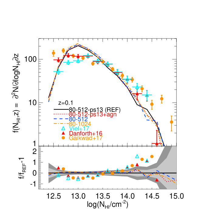

Figure 3 displays the comparison between the CDDF, defined as the number of absorbers per unit log column density per unit redshift, , from the Sherwood models and the COS observations described by V17 at (see also figure 1 in V17). Note that only the 80-512-ps13+agn model was examined in detail by V17; in this work we present a comparison of the additional Sherwood models in which star formation, feedback and numerical resolution have been changed while other parameters remain fixed. We also display the independent measurements of the CDDF from Danforth et al. (2016) (red triangles) and Gaikwad et al. (2017a) (orange circles), although we caution that differences in the line fitting methodologies used in these studies will bias any direct comparison with our simulations.
The simulations fail to capture the correct number of absorbers at , by as much as a factor at . Note that the simulations are well converged with mass resolution – this may be assessed by comparing the 80-512 (blue dashed curve) and 80-1024 (orange dot-dashed curve) models. However, the CDDF is very sensitive to the signal-to-noise and spectral resolution at low column densities (cf. Figure 4 where S/N and FWHM=), and the observational data are incomplete at . This discrepancy therefore reflects differences between the true noise on the data and the idealised, uniform noise added to the mock spectra and is probably not significant. In contrast, the agreement between the V17 data and simulations at is within the uncertainty from sample variance, shown by the grey shading in the lower panel. At , however, the number of absorbers are underpredicted by a factor and the slope of the observed CDDF is shallower than the simulated prediction. A similar discrepancy was present in the recent analysis by Shull et al. (2015) using simulations performed with the Eulerian hydrodynamical code enzo, as well as in the study by Gurvich et al. (2017) with the moving mesh code Arepo, suggesting this discrepancy is not unique to P-Gadget-3 simulations. In contrast Gaikwad et al. (2017b) recently found better agreement with the CDDF at using Gadget-2 adiabatic hydrodynamical simulations post-processed to incorporate radiative cooling, photo-heating and ionisation. Note, however, the effect of gas pressure on the Hdistribution will not be correctly captured in these models, complicating interpretation of this result.
Lastly, it is clear that the various feedback scenarios explored by the simulations impact very little overall on the CDDF at low column densities, particularly at . Outflows have a similarly small impact on the low column Ly forest at ; these systems are associated with the diffuse IGM rather than circumgalactic gas (Theuns et al., 2002; Viel et al., 2013, and see Section 4). Any differences between the feedback models are within the expected 1 sample variance.
This is further emphasised in Figure 4 where we examine the Ly absorption systems at column densities at . Note that we adopt S/N per pixel and a instrument resolution here. The lower panels display the residual with respect to the 80-512-ps13 model, and grey shading shows the Poisson error. The QUICKLYA method (80-512, blue dashed-line) agrees well with the more sophisticated sub-grid physics models for weak absorption systems with at and at . However, higher column density lines are either underpredicted or absent relative to the other models. Multi-phase star formation and stellar feedback (80-512-ps13, black curve) results in a factor of 2-5 more absorption systems at . A similar result was noted by Bolton et al. (2017) for the CDDF at , although the Hcolumn density threshold where QUICKLYA underpredicted the CDDF was higher, . The lack of absorbers is in part because of missing cold dense gas in the QUICKLYA model, but also because winds redistribute gas into the diffuse IGM and introduce peculiar velocities that can increase the equivalent widths of the lines (Davé et al., 2010; Meiksin et al., 2015).
Finally, including AGN feedback in the Sherwood models yields similar results for the CDDF relative to the stellar feedback only model, except at where the incidence of high column density systems is slightly lower (although the total number of absorbers here is small). A stronger effect was noted by Gurvich et al. (2017), who found that the more vigorous AGN feedback in the Illustris simulation suppresses the CDDF at – by a factor of two due to changes in the density and temperature of the gas associated with these absorbers. The higher temperatures reduce the Ly opacity by lowering the radiative recombination rate and (for ) collisionally ionising the gas. In contrast, Tepper-García et al. (2012, see their figure C1) find stellar and AGN feedback have a negligible effect on the CDDF at using simulations drawn from the OWLS project (Schaye et al., 2010). These differences likely reflect variations in the sub-grid physics, as the precise impact of feedback will depend on how efficiently gas is ejected from dark matter haloes.
In contrast to the present study, Tepper-García et al. (2012) also found reasonably good agreement with the HCDDF measurement at from Lehner et al. (2007) based on an earlier compilation of FUSE (Far Ultraviolet Spectroscopic Explorer, FWHM) and HST/STIS (Space Telescope Imaging Spectrograph, FWHM) observations at . However, the models in Tepper-García et al. (2012) underpredicted the incidence of saturated lines at ; their Ly only line fits underestimated the column density of these absorbers since the Lehner et al. (2007) HST/STIS data are obtained from Ly and higher order Lyman lines. The Lehner et al. (2007) HCDDF furthermore only includes absorbers with velocity widths and relative errors less than 40 per cent on and (Lehner et al., 2008, i.e. figure 14 in). We have confirmed we obtain similar agreement with the Lehner et al. (2007) CDDF measurements and our simulations (for and FWHM=) to that obtained by Tepper-García et al. (2012) when selecting only absorbers with .
3.2 The velocity width distribution


We next turn to consider the distribution of Ly line velocity widths, . Figure 5 displays a comparison between the V17 COS measurements and simulations at . We again show the independent measurements from Danforth et al. (2016) (red triangles) and Gaikwad et al. (2017a) (orange circles) for comparison. Overall, the models slightly underpredict the incidence of broad lines at – and overpredict at , although generally the data lie within the expected 95 per cent scatter arising from sample variance in the reference model. It is important to note, however, that unlike the CDDF (where the effect of feedback is comparable to or smaller than the effect of mass resolution) the line widths are not well converged with mass resolution (see also the Appendix later). The distribution from the 80-1024 simulation (orange dot-dashed curve) differs significantly from the 80-512 model (blue dashed curve), particularly at , with a median value of (cf. for the 80-512 model and for the COS data). Higher resolution simulations will therefore predict line widths that are narrower than observed. As pointed out by V17, this suggests there may be additional physics that broadens the absorption lines that is not incorporated into the simulations at present.
We may nevertheless still examine the relative difference between the different feedback models. The incorporation of multi-phase star formation and supernovae-driven winds (black curve) makes very little difference compared to the QUICKLYA model. The addition of AGN feedback (red dotted curve) also has a small effect, increasing the number of broad lines at with a median22 2 This is consistent with V17, who reported an increase by roughly in the median b-parameter when including AGN feedback. Note that V17 incorrectly reported this quantity as the peak of the velocity width distribution rather than the median. b-parameter .
In comparison to earlier work, Davé et al. (2010) also reported a small difference of in the median values predicted by their constant wind and momentum-driven wind models at . However, their velocity widths are generally higher then we find here, with a median value of . The mass resolution of their simulations is around factor of two higher than this work () although performed in smaller volumes . This difference is therefore most likely because Davé et al. (2010) do not deconvolve their Voigt profile fits with the instrument profile (see the first paragraph in section 4 of that paper). Tepper-García et al. (2012) similarly find that AGN feedback produces a small increase in the typical Ly line widths at using the OWLS simulations, and report a median b-parameter of from mock spectra with FWHM= and a S/N per pixel. This is similar to the value of we obtain from our AGN feedback (80-512-ps13+agn) model using the same signal-to-noise and instrument resolution. As Tepper-García et al. (2012) also use SPH simulations performed at slightly lower mass resolution compared to this work (), their line widths will be similarly under-resolved. More recently, Gaikwad et al. (2017b) also found their simulated velocity width distribution predicts lines that are narrower than the COS data. It is possible that the lack of any coupling between radiative cooling, photo-ionisation and the hydrodynamical response of the gas in their simulations may exaggerate this difference further, however.
The impact of feedback on the velocity distribution at is displayed in Figure 6, for FWHM and per pixel. Again it is clear that the velocity width distribution is not converged with mass resolution. By comparing the 80-1024 (orange dot dashed line) and 80-512 (blue dashed line) the line widths differ significantly at . This implies a comparison between simulations and observations requires a mass resolution of at least . However, as for the CDDF, the simulations with varying sub-grid physics performed at the same mass resolution are very similar. The only exception is at when hot gas from AGN feedback produces slightly broader lines.
3.3 The evolution of number density of absorbers
Lastly we examine the number of Habsorbers per unit redshift, . Figure 7 displays for low (, upper panel) and high (, lower panel) column density absorbers, overlaid with a compilation33 3 The individual measurements are from Hu et al. (1995); Lu et al. (1996); Kim et al. (1997); Kirkman & Tytler (1997); Savaglio et al. (1999); Kim et al. (2001); Sembach et al. (2004); Williger et al. (2006); Aracil et al. (2006); Janknecht et al. (2006); Lehner et al. (2007); Williger et al. (2010). of observational data from Kim et al. (2013). In this instance we do not attempt to match the resolution and signal-to-noise of the simulations to the data compilation, which was obtained with a variety of instruments. We instead use FWHM and S/N per pixel and assume the HM01 UVB for emission from star forming galaxies and quasars. We also show the more recent COS measurements44 4 Note the Danforth et al. (2016) measurements in the upper panel of Fig. 7 are for the slightly different column density range , rather than used for the Kim et al. (2013) data compilation. from Danforth et al. (2016) at . These are formally consistent with the earlier data compilation at , but with an increased incidence of lines at . Note also we use Ly only fits for comparison to the observations, which may complicate the comparison to the stronger, saturated lines with column densities inferred using higher order Lyman lines. We have therefore tested this by also directly integrating the Hnumber densities along the simulated sight-lines to obtain (Gurvich et al., 2017, see also). This procedure yields similar results to the Voigt profile fits.
The number of low column density Ly forest absorbers (top panel) is not sensitive to the differences in star formation and feedback prescriptions in the models. This is consistent with the CDDF, where galactic winds and AGN feedback do not significantly impact on the gas distribution at the low column densities that probe the diffuse IGM (Davé et al., 2010, see also). The simulations are in good agreement with the observational data at , but underpredict the number of weak lines at . To investigate this further, we have rescaled the mean transmission in the 80-512-ps13 model to at (blue triangle), which V17 find provides a better match to CDDF at . The improved agreement again demonstrates this discrepancy is due to the uncertain UVB amplitude; the HM01 model overpredicts the Hphoto-ionisation rate at .
In contrast to the low column density systems, the simulated predictions for higher column density Ly forest absorbers exhibit some differences with the choice of star formation and feedback model at . The 80-512-ps13 model produces a factor of higher relative to 80-512 at , with the AGN feedback intermediate between the two. However, all models fail to reproduce the observational data at . Rescaling the mean transmission at slightly improves agreement but does not remove the discrepancy. In combination with the CDDF, this strongly suggests the simulations are not correctly capturing the saturated Ly absorption systems that are still optically thin to Lyman continuum radiation.
4 Identifying the gas responsible for low redshift Ly forest absorbers
| Name | Model | Diffuse | WHIM | Hot Halo | Condensed | Stars |
|---|---|---|---|---|---|---|
| K | K | K | ||||
| 80-512 | 36.5 | 21.3 | 17.1 | 0.9 | 24.2 | |
| 80-512-ps13 | 36.6 | 24.3 | 22.4 | 9.1 | 7.7 | |
| 80-512-ps13+agn | 36.5 | 36.9 | 20.0 | 3.3 | 3.3 | |
| 80-512 | 51.7 | 15.4 | 12.6 | 1.9 | 18.4 | |
| 80-512-ps13 | 51.9 | 17.0 | 16.3 | 10.6 | 4.3 | |
| 80-512-ps13+agn | 51.6 | 19.2 | 17.7 | 8.5 | 3.0 | |
| 80-512 | 61.8 | 11.3 | 8.9 | 2.8 | 15.1 | |
| 80-512-ps13 | 62.0 | 12.3 | 11.3 | 11.5 | 2.8 | |
| 80-512-ps13+agn | 62.0 | 12.7 | 11.7 | 11.1 | 2.4 |


In order to more closely examine the physical origin of the absorption in our models and assess the effect of feedback, we consider the typical temperature and density of gas in the QUICKLYA model (80-512) and the Puchwein & Springel (2013) energy driven winds model with (80-512-ps13+agn) and without (80-512-ps13) AGN feedback. We have divided the gas into four categories based on temperature, , and normalised density thresholds, , following Davé et al. (2010). These are i) diffuse gas (K) ii) the warm-hot IGM (WHIM, K) iii) hot halo gas (K, and iv) condensed gas (K). In Table 2, the percentage of the total baryon mass in each category is shown at and where and , respectively (Davé et al., 2010, here is computed using equations 1 and 2 in). We have also included the percentage of gas that has been converted into collsionless star particles.
The redshift evolution of gas in the diffuse phase is very similar for all models, with no noticeable difference due to feedback. This diffuse gas follows a power law temperature-density relationship, (see Figure 1). However, there is a significant increase in the mass fraction in the WHIM for the model with AGN feedback at , with a corresponding decrease in the condensed phase fraction and stellar mass. Including multi-phase star formation and stellar feedback produces more gas in the hot halo and condensed phases compared to the QUICKLYA model at . In contrast, the QUICKLYA model produces significantly more stars at and – while capturing the diffuse IGM reasonably well – will produce unreliable results for gravitationally bound gas at .
The mass fractions for the 80-512-ps13 model are broadly similar to the “vzw” momentum driven winds model described in Davé et al. (2010), with slightly more ( per cent) gas in the dense phases with . There is also reasonable agreement between the 80-512-ps13 model and the post-processed adiabatic simulations described by Gaikwad et al. (2017a) at , with around 4 per cent more (less) gas in the WHIM (hot halo) phase. This suggests the bulk of the hot gas with in the models without AGN feedback is produced by gravitational infall. The largest difference is the condensed phase which contains 18.8 per cent of the mass at in Gaikwad et al. (2017a); this is because dense gas is not converted into stars in their adiabatic simulations.
The connection between the density and temperature of the gas and the column density and velocity widths of the Ly absorbers at is summarised in Figure 8. Along each simulated line of sight we have computed the optical depth weighted temperature, , and density, , where and is optical depth at the pixel in real space contributing to the pixel in velocity space (Schaye et al., 1999). We then associate and with and at the location of the line centres identified by VPFIT. This approach takes redshift space distortions due to the peculiar motion of the gas into account. As before, following V17 we only consider systems with relative errors less then 50 per cent on and .
The top panel of Figure 8 displays the relationship between and in the simulations. The data are coloured according to their velocity widths. The red dashed line shows the power-law relationship between and predicted by Schaye (2001), assuming the typical size of an Habsorber is the local Jeans scale:
| (1) |
Here is the Hphoto-ionisation rate (where at in the 80-512-ps13 simulation for ) and is the gas temperature.
This provides a good description of the scaling between gas density and Hcolumn density (Davé et al., 1999; Davé et al., 2010; Tepper-García et al., 2012, see also). The majority of the absorption lines at – correspond to gas densities – in the simulations (V17), with typical velocity widths of –. In all models there are a small number of broad lines, , with column densities – that are associated with hot gas in the WHIM with – (Tepper-García et al., 2012, see also). The effect of feedback on the diffuse, low column density gas is rather subtle; there are slightly more broad lines lying above the correlation for the AGN feedback model, consistent with additional heating. Although there is significantly more hot gas in the WHIM by mass at when including AGN feedback, much of this is also collisionally ionised. In all instances, however, the higher column density systems, correspond to gas densities at . The simulations fail to correctly capture the number density of these systems, some of which are at densities associated with circumgalactic gas.
The lower panel in Figure 8 shows the corresponding values of at the line centres against the velocity widths. The red dashed line displays the expected velocity width under the assumption of pure thermal broadening:
| (2) |
In general, although the minimum line widths trace the expectation for thermal broadening, most of the absorbers are significantly broader, particularly for low column density lines originating from low density gas (see also Garzilli et al., 2015, for a recent discussion at ). Many of the absorbers are therefore broadened through the additional effects of gas pressure (i.e. Jeans smoothing). The absorbers with – are associated with gas with a broad range of temperatures, but most are in the range –. The velocity widths of these lines remain too narrow with respect to the COS data. Again, the effect of stellar and AGN feedback on the temperature of the absorbers is small.
5 Conclusions
We have investigated the impact of different feedback prescriptions on the properties of the low redshift Ly forest, using a selection of hydrodynamical simulations drawn from the Sherwood simulation suite. The simulations adopt stellar feedback, AGN feedback and a simplified scheme for modelling the low column density Ly forest that converts all gas with and into collisionless star particles. We have examined the CDDF, velocity width distribution, the redshift evolution in the line number density, , and the relationship between the column density, velocity widths, and the underlying gas density and temperature.
Our analysis confirms the finding by V17 that the velocity widths of simulated Ly absorption lines with gas densities – are too narrow when compared with COS data. We also stress that this difference will be exacerbated further for simulations performed at higher mass resolution than considered here; the line widths are under-resolved at our fiducial resolution of (see also the Appendix). We also find that absorbers with column densities , which correspond to gas with in our simulations, are underestimated, in agreement with earlier work (Shull et al., 2015; Gurvich et al., 2017).
On the other hand, using simulations that vary the feedback prescription while keeping other parameters fixed, we find that the impact of galactic winds and AGN feedback is generally very modest. AGN feedback only impacts on the Ly absorbers at very low redshift, , by producing some broader lines and slightly reducing the incidence of systems with with respect to a model with only stellar feedback. There is no noticeable impact on the CDDF due to stellar or AGN feedback at . Furthermore, we find a simplified scheme that ignores feedback and star formation altogether adequately capture the properties of absorption lines with , although the incidence of stronger systems is underestimated compared to models that include feedback. Similarly, the Ly line number density and its evolution with redshift, , is in good agreement with observational data for low column density systems, , once the amplitude of the UVB is rescaled to match the CDDF. In contrast, for high column density systems, , the simulations underpredict the incidence of absorbers at and by a factor of and , respectively.
This demonstrates that stellar and AGN feedback – as currently implemented in our simulations – have a limited impact on the Ly forest. We conclude that resolving the discrepancy between COS data and the simulations requires an increase in the temperature of gas with –, either through (i) additional Hephoto-heating at , (ii) additional fine-tuned feedback that ejects overdense gas into the IGM at just the right temperature for it to still contribute significantly to the Ly forest or alternatively (iii) a larger, currently unresolved turbulent component to the line widths (Oppenheimer & Davé, 2009; Iapichino et al., 2013; Gaikwad et al., 2017b). Note, however, the first possibility would require a UVB with a harder spectrum at , potentially producing gas temperatures that are too high with respect to existing observational constraints from the Ly forest at (Becker et al., 2011; Boera et al., 2014; Bolton et al., 2014). Our results provide further motivation for studying the impact of state-of-the-art feedback models on the properties of the low redshift Ly forest.
Acknowledgments
The hydrodynamical simulations used in this work were performed with supercomputer time awarded by the Partnership for Advanced Computing in Europe (PRACE) 8th Call. We acknowledge PRACE for awarding us access to the Curie supercomputer, based in France at the Tre Grand Centre de Calcul (TGCC). This work also made use of the DiRAC High Performance Computing System (HPCS) and the COSMOS shared memory service at the University of Cambridge. These are operated on behalf of the STFC DiRAC HPC facility. This equipment is funded by BIS National E-infrastructure capital grant ST/J005673/1 and STFC grants ST/H008586/1, ST/K00333X/1. We thank Volker Springel for making P-GADGET-3 available. FN is supported by a Vice-Chancellor’s Scholarship for Research Excellence. JSB acknowledges the support of a Royal Society University Research Fellowship. MV and TSK are supported by the FP7 ERC grant “cosmoIGM” and the INFN/PD51 grant. TSK also acknowledges the NSF-AST118913. MGH and EP acknowledge support from the FP7 ERC Grant Emergence-320596, and EP gratefully acknowledges support by the Kavli Foundation. DS acknowledges support by the STFC and the ERC starting grant 638707 “Black holes and their host galaxies: co-evolution across cosmic time”.
References
- Adams et al. (2011) Adams J. J., Uson J. M., Hill G. J., MacQueen P. J., 2011, ApJ, 728, 107
- Aracil et al. (2006) Aracil B., Tripp T. M., Bowen D. V., Prochaska J. X., Chen H.-W., Frye B. L., 2006, MNRAS, 367, 139
- Bahcall et al. (1993) Bahcall J. N., et al., 1993, ApJS, 87, 1
- Becker et al. (2011) Becker G. D., Bolton J. S., Haehnelt M. G., Sargent W. L. W., 2011, MNRAS, 410, 1096
- Boera et al. (2014) Boera E., Murphy M. T., Becker G. D., Bolton J. S., 2014, MNRAS, 441, 1916
- Bolton et al. (2014) Bolton J. S., Becker G. D., Haehnelt M. G., Viel M., 2014, MNRAS, 438, 2499
- Bolton et al. (2017) Bolton J. S., Puchwein E., Sijacki D., Haehnelt M. G., Kim T.-S., Meiksin A., Regan J. A., Viel M., 2017, MNRAS, 464, 897
- Carswell & Webb (2014) Carswell R. F., Webb J. K., 2014, VPFIT: Voigt profile fitting program, Astrophysics Source Code Library (ascl:1408.015)
- Cen & Ostriker (1999) Cen R., Ostriker J. P., 1999, ApJ, 514, 1
- Danforth et al. (2016) Danforth C. W., et al., 2016, ApJ, 817, 111
- Davé et al. (1999) Davé R., Hernquist L., Katz N., Weinberg D. H., 1999, ApJ, 511, 521
- Davé et al. (2010) Davé R., Oppenheimer B. D., Katz N., Kollmeier J. A., Weinberg D. H., 2010, MNRAS, 408, 2051
- Faucher-Giguère et al. (2009) Faucher-Giguère C., Lidz A., Zaldarriaga M., Hernquist L., 2009, ApJ, 703, 1416
- Fumagalli et al. (2017) Fumagalli M., Haardt F., Theuns T., Morris S. L., Cantalupo S., Madau P., Fossati M., 2017, MNRAS, 467, 4802
- Gaikwad et al. (2017a) Gaikwad P., Khaire V., Choudhury T. R., Srianand R., 2017a, MNRAS, 466, 838
- Gaikwad et al. (2017b) Gaikwad P., Srianand R., Choudhury T. R., Khaire V., 2017b, MNRAS, 467, 3172
- Garzilli et al. (2015) Garzilli A., Theuns T., Schaye J., 2015, MNRAS, 450, 1465
- Gnedin & Hui (1998) Gnedin N. Y., Hui L., 1998, MNRAS, 296, 44
- Green et al. (2012) Green J. C., et al., 2012, ApJ, 744, 60
- Gurvich et al. (2017) Gurvich A., Burkhart B., Bird S., 2017, ApJ, 835, 175
- Haardt & Madau (2001) Haardt F., Madau P., 2001, in Clusters of Galaxies and the High Redshift Universe Observed in X-rays, Neumann, D. M. & Tran, J. T. V. ed., astro-ph/0106018.
- Haardt & Madau (2012) Haardt F., Madau P., 2012, ApJ, 746, 125
- Hu et al. (1995) Hu E. M., Kim T.-S., Cowie L. L., Songaila A., Rauch M., 1995, AJ, 110, 1526
- Iapichino et al. (2013) Iapichino L., Viel M., Borgani S., 2013, MNRAS, 432, 2529
- Janknecht et al. (2006) Janknecht E., Reimers D., Lopez S., Tytler D., 2006, A&A, 458, 427
- Khaire & Srianand (2015) Khaire V., Srianand R., 2015, MNRAS, 451, L30
- Khaire et al. (2016) Khaire V., Srianand R., Choudhury T. R., Gaikwad P., 2016, MNRAS, 457, 4051
- Kim et al. (1997) Kim T.-S., Hu E. M., Cowie L. L., Songaila A., 1997, AJ, 114, 1
- Kim et al. (2001) Kim T.-S., Cristiani S., D’Odorico S., 2001, A&A, 373, 757
- Kim et al. (2007) Kim T.-S., Bolton J. S., Viel M., Haehnelt M. G., Carswell R. F., 2007, MNRAS, 382, 1657
- Kim et al. (2013) Kim T.-S., Partl A. M., Carswell R. F., Müller V., 2013, A&A, 552, A77
- Kirkman & Tytler (1997) Kirkman D., Tytler D., 1997, ApJ, 484, 672
- Kirkman et al. (2007) Kirkman D., Tytler D., Lubin D., Charlton J., 2007, MNRAS, 376, 1227
- Kollmeier et al. (2014) Kollmeier J. A., et al., 2014, ApJ, 789, L32
- Lehner et al. (2007) Lehner N., Savage B. D., Richter P., Sembach K. R., Tripp T. M., Wakker B. P., 2007, ApJ, 658, 680
- Lehner et al. (2008) Lehner N., Savage B. D., Richter P., Sembach K. R., Tripp T. M., Wakker B. P., 2008, ApJ, 674, 613
- Lewis et al. (2000) Lewis A., Challinor A., Lasenby A., 2000, ApJ, 538, 473
- Lu et al. (1996) Lu L., Sargent W. L. W., Womble D. S., Takada-Hidai M., 1996, ApJ, 472, 509
- Madau & Haardt (2015) Madau P., Haardt F., 2015, ApJ, 813, L8
- McQuinn (2016) McQuinn M., 2016, ARA&A, 54, 313
- Meiksin (2009) Meiksin A. A., 2009, Reviews of Modern Physics, 81, 1405
- Meiksin et al. (2015) Meiksin A., Bolton J. S., Tittley E. R., 2015, MNRAS, 453, 899
- Oppenheimer & Davé (2009) Oppenheimer B. D., Davé R., 2009, MNRAS, 395, 1875
- Pachat et al. (2016) Pachat S., Narayanan A., Muzahid S., Khaire V., Srianand R., Wakker B. P., Savage B. D., 2016, MNRAS, 458, 733
- Paschos et al. (2009) Paschos P., Jena T., Tytler D., Kirkman D., Norman M. L., 2009, MNRAS, 399, 1934
- Planck Collaboration et al. (2014) Planck Collaboration et al., 2014, A&A, 571, A31
- Puchwein & Springel (2013) Puchwein E., Springel V., 2013, MNRAS, 428, 2966
- Puchwein et al. (2015) Puchwein E., Bolton J. S., Haehnelt M. G., Madau P., Becker G. D., Haardt F., 2015, MNRAS, 450, 4081
- Rahmati et al. (2013) Rahmati A., Pawlik A. H., Raicevic M., Schaye J., 2013, MNRAS, 430, 2427
- Rauch et al. (1997) Rauch M., et al., 1997, ApJ, 489, 7
- Richter et al. (2006) Richter P., Fang T., Bryan G. L., 2006, A&A, 451, 767
- Ricotti et al. (2000) Ricotti M., Gnedin N. Y., Shull J. M., 2000, ApJ, 534, 41
- Rollinde et al. (2013) Rollinde E., Theuns T., Schaye J., Pâris I., Petitjean P., 2013, MNRAS, 428, 540
- Savaglio et al. (1999) Savaglio S., et al., 1999, ApJ, 515, L5
- Schaye (2001) Schaye J., 2001, ApJ, 559, 507
- Schaye et al. (1999) Schaye J., Theuns T., Leonard A., Efstathiou G., 1999, MNRAS, 310, 57
- Schaye et al. (2000) Schaye J., Theuns T., Rauch M., Efstathiou G., Sargent W. L. W., 2000, MNRAS, 318, 817
- Schaye et al. (2010) Schaye J., et al., 2010, MNRAS, 402, 1536
- Scott et al. (2002) Scott J., Bechtold J., Morita M., Dobrzycki A., Kulkarni V. P., 2002, ApJ, 571, 665
- Sembach et al. (2004) Sembach K. R., Tripp T. M., Savage B. D., Richter P., 2004, ApJS, 155, 351
- Shull et al. (2012) Shull J. M., Smith B. D., Danforth C. W., 2012, ApJ, 759, 23
- Shull et al. (2014) Shull J. M., Danforth C. W., Tilton E. M., 2014, ApJ, 796, 49
- Shull et al. (2015) Shull J. M., Moloney J., Danforth C. W., Tilton E. M., 2015, ApJ, 811, 3
- Sijacki et al. (2007) Sijacki D., Springel V., Di Matteo T., Hernquist L., 2007, MNRAS, 380, 877
- Springel (2005) Springel V., 2005, MNRAS, 364, 1105
- Springel & Hernquist (2003) Springel V., Hernquist L., 2003, MNRAS, 339, 289
- Springel et al. (2005) Springel V., et al., 2005, Nature, 435, 629
- Tepper-García (2006) Tepper-García T., 2006, MNRAS, 369, 2025
- Tepper-García et al. (2012) Tepper-García T., Richter P., Schaye J., Booth C. M., Dalla Vecchia C., Theuns T., 2012, MNRAS, 425, 1640
- Theuns et al. (1998a) Theuns T., Leonard A., Efstathiou G., 1998a, MNRAS, 297, L49
- Theuns et al. (1998b) Theuns T., Leonard A., Efstathiou G., Pearce F. R., Thomas P. A., 1998b, MNRAS, 301, 478
- Theuns et al. (2002) Theuns T., Viel M., Kay S., Schaye J., Carswell R. F., Tzanavaris P., 2002, ApJ, 578, L5
- Tilton et al. (2012) Tilton E. M., Danforth C. W., Shull J. M., Ross T. L., 2012, ApJ, 759, 112
- Upton Sanderbeck et al. (2016) Upton Sanderbeck P. R., D’Aloisio A., McQuinn M. J., 2016, MNRAS, 460, 1885
- Viel et al. (2004) Viel M., Haehnelt M. G., Springel V., 2004, MNRAS, 354, 684
- Viel et al. (2013) Viel M., Schaye J., Booth C. M., 2013, MNRAS, 429, 1734
- Viel et al. (2017) Viel M., Haehnelt M. G., Bolton J. S., Kim T.-S., Puchwein E., Nasir F., Wakker B. P., 2017, MNRAS, 467, L86
- Vogelsberger et al. (2014) Vogelsberger M., et al., 2014, MNRAS, 444, 1518
- Wakker et al. (2015) Wakker B. P., Hernandez A. K., French D. M., Kim T.-S., Oppenheimer B. D., Savage B. D., 2015, ApJ, 814, 40
- Weymann et al. (1998) Weymann R. J., et al., 1998, ApJ, 506, 1
- Williger et al. (2006) Williger G. M., Heap S. R., Weymann R. J., Davé R., Ellingson E., Carswell R. F., Tripp T. M., Jenkins E. B., 2006, ApJ, 636, 631
- Williger et al. (2010) Williger G. M., et al., 2010, MNRAS, 405, 1736
Appendix A numerical convergence
We have performed convergence tests with mass resolution and box size for the Ly forest CDDF and velocity width distribution at the redshifts considered in this paper. These are displayed in Figures 9-12. The CDDF is well converged with mass resolution and box size within the range . However, at () the number of lines are over (under) estimated at lower mass resolution. This suggests that numerical resolution is unlikely to be the cause of the discrepancy between the COS observations and our simulations at .
In Figure 11, however, it is clear that mass resolution significantly impacts on the velocity width distributions, with line widths that are systematically overestimated at our fiducial resolution of (80-512). A mass resolution of at least is required for an acceptable level of convergence. This means the discrepancy between the COS observations of the velocity width distribution will be even larger for higher resolution simulations. The Ly line width distribution is generally well converged with box size, as shown Figure 12, with the exception of lines at in the box.
Finally, Figures 11-12 and Table 3 display convergence tests for the volume weighted IGM thermal state with box size and mass resolution. The results are well converged with box size, but demonstrate the temperature of the IGM at mean density is overestimated by – per cent at our fiducial resolution (80-512). We have checked, however, that the mass weighted temperature obtained from the gas particles is well converged with mass resolution, suggesting this difference originates from the larger smoothing lengths used in the lower resolution models. Note also that , shown in the middle panels of Figures 11-12, corresponds to , and therefore reflects the convergence of both and . Additionally, we observe from Table 3 that as mass resolution is increased using the QUICKLYA model, a greater proportion by mass of the baryons are converted to collisionless star particles. Note, however, this is already a significant overestimate and the results of the QUICKLYA model will be unreliable for gas at .


| Name | Model | Diffuse | WHIM | Hot Halo | Condensed | Stars |
|---|---|---|---|---|---|---|
| K | K | K | ||||
| 80-1024 | 35.0 | 20.1 | 15.3 | 0.7 | 28.8 | |
| 80-512 | 36.5 | 21.3 | 17.1 | 0.9 | 24.2 | |
| 80-256 | 39.7 | 22.6 | 20.0 | 1.2 | 16.6 | |
| 40-512 | 34.6 | 20.5 | 15.3 | 0.8 | 28.8 | |
| 20-256 | 35.3 | 19.4 | 15.2 | 0.7 | 29.3 | |
| 80-1024 | 49.6 | 14.5 | 11.1 | 1.6 | 23.2 | |
| 80-512 | 51.7 | 15.4 | 12.6 | 1.9 | 18.4 | |
| 80-256 | 55.4 | 16.4 | 14.9 | 2.1 | 11.2 | |
| 40-512 | 49.2 | 15.0 | 11.1 | 1.5 | 23.2 | |
| 20-256 | 49.7 | 13.5 | 11.5 | 1.6 | 23.7 | |
| 80-1024 | 59.3 | 10.7 | 7.7 | 2.3 | 20.0 | |
| 80-512 | 61.8 | 11.3 | 8.9 | 2.8 | 15.1 | |
| 80-256 | 65.7 | 12.3 | 10.6 | 2.9 | 8.4 | |
| 40-512 | 58.9 | 11.1 | 7.8 | 2.2 | 19.9 | |
| 20-256 | 59.2 | 10.2 | 7.9 | 2.3 | 20.4 |