跳到论文正文
W Papers独立论文阅读器 arXiv:1706.04781 论文正文 计算阅读时间 · 0%
引用这篇论文根据当前论文元数据生成,正式投稿前建议核对。


License: arXiv.org perpetual non-exclusive license
arXiv:1706.04781v2 [stat.CO] 18 Jun 2017

Generalized Bouncy Particle Sampler

Changye Wu ††thanks: CEREMADE, Université Paris-Dauphine PSL, France. wu@ceremade.dauphine.fr    Christian Robert ††thanks: Université Paris Dauphine PSL, CREST, France and University of Warwick, UK. xian@ceremade.dauphine.fr
Abstract

As a special example of piecewise deterministic Markov process, bouncy particle sampler is a rejection-free, irreversible Markov chain Monte Carlo algorithm and can draw samples from target distribution efficiently. We generalize bouncy particle sampler in terms of its transition dynamics. In BPS, the transition dynamic at event time is deterministic, but in GBPS, it is random. With the help of this randomness, GBPS can overcome the reducibility problem in BPS without refreshment.

1 Introduction

As a powerful sampling technique, Markov chain Monte Carlo (MCMC) method has been widely used in computational statistics and is now a standard tool in Bayesian inference, where posterior distribution is often intractable analytically, known up to a constant. However, almost all existing MCMC algorithms, such as Metropolis-Hastings algorithm (MH), Hamiltonian Monte Carlo (HMC) and Metropolis adjusted Langevin algorithm (MALA), are based on detailed balance condition, dating back to ([16], [12]). Recently, a novel type of MCMC method — piecewise deterministic Markov process (PDMP) — appeared in computational statistics, method that is generally irreversible, meaning a violation of the detailed balance condition. The theory of PDMP is developed by ([8], [9]), while its quite remarkable applications on computational statistics are implemented by ([6], [2], [4]).

Compared with traditional MCMC algorithms, PDMP is rejection-free, which means that there is no waste of proposal samples. Based on detailed balance condition, traditional MCMC algorithms are reversible. However, some theoretic work and numerical experiments ([13], [22], [7], [3]) have shown that irreversible Markov chain can outperform reversible MCMC with respect to mixing rate and asymptotic variance. PDMP is a typically irreversible Markov chain, which is of interest to investigate. Bouncy particle sampler (BPS) generates a special piecewise deterministic Markov chain, originating in [19] and being explored by [6]. Zig-zag process sampler [4] is another PDMP example and [10] unifies the BPS and zig-zag process sampler in the framework of PDMP. Besides, MCMC algorithms are difficult to scale, since computing each MH acceptance ratio needs to sweep over the whole data set. However, according to their special structures, BPS and zig-zag process sampler are easy to scale for big data. Except PDMP style MCMC algorithms, almost all other existing scalable MCMC algorithms (such as, [21], [18], [23], [17], [20], [1]), are approximate, not exact, which do not admit the target distribution as their invariant distribution.

In this article, we generalize bouncy particle sampler – generalized bouncy particle sampler (GBPS) – which can be treated as an extension of BPS and zig-zag process sampler. In BPS, the transition dynamic at event time is deterministic. In opposition, the transition dynamic in GBPS is random with respect to some distribution. In zig-zag process sampler, we decompose the velocity with respect to some fixed coordinate system, while in GBPS, we use a moving coordinate system to decompose the velocity. Besides, the main gain of GBPS compared with BPS is that there is no parameter to tune. In fact, for BPS, in order to overcome the reducibility problem, we need to add a refreshment Poisson process to refresh the velocity occasionally, which needs to be tuned to balance the efficiency and accuracy. But for GBPS, the randomness of refreshment is incorporated into the transition dynamics and there is no parameter to tune.

This paper is organized as follows: we introduce piecewise deterministic Markov process and bouncy particle sampler in section 2, followed by the introduction of generalized bouncy particle sampler (GBPS) and its implementation issues in section 3. In section 4, we present three numerical experiments of GBPS. At last, we discuss some questions and conclude in section 5.

2 Piecewise Deterministic Markov Process

In this section, suppose π⁡(𝕩)\pi(\mathbb{x}) be the target distribution, where 𝕩∈ℝd\mathbb{x}\in\mathbb{R}^{d}. We introduce an auxiliary variable, 𝕧∈ℝd\mathbb{v}\in\mathbb{R}^{d}, called velocity, which is restricted to be of unit length, ‖𝕧‖2=1\|\mathbb{v}\|_{2}=1. Denote 𝕫=(𝕩,𝕧)∈ℝd×Sd−1\mathbb{z}=(\mathbb{x},\mathbb{v})\in\mathbb{R}^{d}\times S_{d-1}. In order to obtain the target, we just need to force π⁡(𝕩)\pi(\mathbb{x}) to be the marginal distribution of π⁡(𝕩,𝕧)\pi(\mathbb{x},\mathbb{v}) with respect to 𝕩\mathbb{x}. Let {𝕫t}\{\mathbb{z}_{t}\} denote a piecewise deterministic Markov chain of 𝕫\mathbb{z} on the augmented space (𝕩,𝕧)∈ℝd×Sd−1(\mathbb{x},\mathbb{v})\in\mathbb{R}^{d}\times S_{d-1}. The dynamics of PDMP consist of three types of dynamics, namely, deterministic dynamic, event occurrence and transition dynamic. Specifically,

  1. 1.

    The deterministic dynamic: between two event times, the Markov process evolves deterministically, according to some partial differential equation:

    d​zt(i)d​t=Ψ(i)(𝕫t),i=1,⋯,2d\frac{dz^{(i)}_{t}}{dt}=\Psi^{(i)}(\mathbb{z}_{t}),\quad i=1,\cdots,2d
  2. 2.

    The event occurrence: the event occurs at the rate: λ⁡(𝕫t)\lambda(\mathbb{z}_{t}).

  3. 3.

    The transition dynamic: At the event time, τ\tau, we denote 𝕫τ−\mathbb{z}_{\tau-} the state prior to τ\tau, then 𝕫τ∼Q(⋅|𝕫τ−)\mathbb{z}_{\tau}\sim Q(\cdot|\mathbb{z}_{\tau-})

Following from ([9], Theorem 26.14), this Markov process’s extension generator is

𝒜​f​(𝕫)=∇f​(𝕫)⋅Ψ⁡(𝕫)+λ⁡(𝕫)​∫ℝd×Sd−1(f⁡(𝕫′)−f⁡(𝕫))​Q​(d​𝕫′,𝕫)\mathcal{A}f(\mathbb{z})=\nabla f(\mathbb{z})\cdot\Psi(\mathbb{z})+\lambda(\mathbb{z})\int_{\mathbb{R}^{d}\times S_{d-1}}\left(f(\mathbb{z}^{\prime})-f(\mathbb{z})\right)Q(d\mathbb{z}^{\prime};\mathbb{z})

2.1 Bouncy Particle Sampler

Bouncy particle sampler (BPS) is a specific piecewise deterministic Markov process, which admits π⁡(𝕩)​d​𝕩⊗d​𝕧\pi(\mathbb{x})d\mathbb{x}\otimes d\mathbb{v} over the state space ℝd×Sd−1\mathbb{R}^{d}\times S_{d-1} as its invariant distribution, by specifying the event rate λ⁡(𝕫)\lambda(\mathbb{z}) and the transition dynamic Q⁡(d​𝕫′,𝕫)Q(d\mathbb{z}^{\prime};\mathbb{z}).

  1. 1.

    The deterministic dynamic:

    d​xt(i)d​t=v(i)t,d​vt(i)d​t=0,i=1,⋯,d\frac{dx^{(i)}_{t}}{dt}=v^{(i)}_{t},\quad\frac{dv^{(i)}_{t}}{dt}=0,\quad i=1,\cdots,d
  2. 2.

    The event occurrence: λ(𝕫t)=max{0,−𝕧t⋅∇logπ(𝕩t)}\lambda(\mathbb{z}_{t})=\max\{0,-\mathbb{v}_{t}\cdot\nabla\log\pi(\mathbb{x}_{t})\}.

  3. 3.

    The transition dynamic: Q(⋅|𝕩,𝕧)=δ(𝕩,P𝕩​𝕧)(⋅)Q(\cdot|\mathbb{x},\mathbb{v})=\delta_{(\mathbb{x},P_{\mathbb{x}}\mathbb{v})}(\cdot), where

    P𝕩𝕧=𝕧−2⟨𝕧,∇log⁡π​(𝕩)⟩⟨∇log⁡π​(𝕩),∇log⁡π​(𝕩)⟩∇logπ(𝕩)P_{\mathbb{x}}\mathbb{v}=\mathbb{v}-2\frac{\langle\mathbb{v},\nabla\log\pi(\mathbb{x})\rangle}{\langle\nabla\log\pi(\mathbb{x}),\nabla\log\pi(\mathbb{x})\rangle}\nabla\log\pi(\mathbb{x})

[6] has shown that BPS admits π⁡(𝕩)​d​𝕩⊗d​𝕧\pi(\mathbb{x})d\mathbb{x}\otimes d\mathbb{v} as its invariant distribution. However, the authors also find that pure BPS (specified above) meets with a reducibility problem and add a reference Poisson process into BPS to overcome it. The workflow of BPS with refreshment is shown in Algorithm 1.

Algorithm 1 Bouncy Particle Sampler
 Initialize: 𝕩0,𝕧0,T0=0\mathbb{x}_{0},\mathbb{v}_{0},T_{0}=0.
 for i=1,2,3,⋯i=1,2,3,\cdots do
  Generate τ∼P​P​(λ⁡(𝕩t,𝕧t))\tau\sim PP(\lambda(\mathbb{x}_{t},\mathbb{v}_{t}))
  Generate τref∼P​P​(λref)\tau^{\text{ref}}\sim PP(\lambda^{\text{ref}})
  if τ≤τref\tau\leq\tau^{\text{ref}} then
   Ti←Ti−1+τT_{i}\leftarrow T_{i-1}+\tau
   𝕩i←𝕩i−1+τ​𝕧i−1\mathbb{x}_{i}\leftarrow\mathbb{x}_{i-1}+\tau\mathbb{v}_{i-1}
   𝕧i←𝕧i−1−2⟨𝕧i−1,∇log⁡π​(𝕩i)⟩⟨∇log⁡π​(𝕩i),∇log⁡π​(𝕩i)⟩∇logπ(𝕩i)\mathbb{v}_{i}\leftarrow\mathbb{v}_{i-1}-2\frac{\langle\mathbb{v}_{i-1},\nabla\log\pi(\mathbb{x}_{i})\rangle}{\langle\nabla\log\pi(\mathbb{x}_{i}),\nabla\log\pi(\mathbb{x}_{i})\rangle}\nabla\log\pi(\mathbb{x}_{i})
  else
   Ti←Ti−1+τrefT_{i}\leftarrow T_{i-1}+\tau^{\text{ref}}
   𝕩i←𝕩i−1+τref​𝕧i−1\mathbb{x}_{i}\leftarrow\mathbb{x}_{i-1}+\tau^{\text{ref}}\mathbb{v}_{i-1}
   𝕧i∼𝒰⁡(Sd−1)\mathbb{v}_{i}\sim\mathcal{U}(S_{d-1})
  end if
 end for

3 Generalized Bouncy Particle Sampler

In BPS, at event time, the velocity changes deterministically. However, we find that the velocity can be changed into other directions, according to some distribution, at event time, which incorporates the randomness of the reference Poisson process in BPS to overcome the reducibility. In this section, we generalize the BPS. Specifically, prior to event time, we decompose the velocity according to the gradient of log⁡π⁡(𝕩)\log{\pi(\mathbb{x})}, flip the parallel subvector and resample the orthogonal subvector with respect to some distribution. The details are as follows:

  1. 1.

    The deterministic dynamic:

    d​xt(i)d​t=v(i)t,d​vt(i)d​t=0,i=1,⋯,d\frac{dx^{(i)}_{t}}{dt}=v^{(i)}_{t},\quad\frac{dv^{(i)}_{t}}{dt}=0,\quad i=1,\cdots,d
  2. 2.

    The event occurrence: λ⁡(𝕫t)=max⁡{0,−⟨𝕧t,∇log⁡π​(𝕩t)⟩}\lambda(\mathbb{z}_{t})=\max\{0,-\langle\mathbb{v}_{t},\nabla\log\pi(\mathbb{x}_{t})\rangle\}.

  3. 3.

    The transition dynamic: Q(d𝕩′,d𝕧′|𝕩,𝕧)=δ{𝕩}(d𝕩′)δ{−𝕧1}(d𝕧1′)𝒩𝕧1⟂(d𝕧2′)Q(d\mathbb{x}^{\prime},d\mathbb{v}^{\prime}|\mathbb{x},\mathbb{v})=\delta_{\{\mathbb{x}\}}(d\mathbb{x}^{\prime})\delta_{\{-\mathbb{v}_{1}\}}(d\mathbb{v}^{\prime}_{1})\mathcal{N}_{\mathbb{v}_{1}^{\perp}}(d\mathbb{v}^{\prime}_{2}), where

    𝕧1=⟨𝕧,∇log⁡π​(𝕩)⟩⟨∇log⁡π​(𝕩),∇log⁡π​(𝕩)⟩∇logπ(𝕩),𝕧2=𝕧−𝕧1\mathbb{v}_{1}=\frac{\langle\mathbb{v},\nabla\log\pi(\mathbb{x})\rangle}{\langle\nabla\log\pi(\mathbb{x}),\nabla\log\pi(\mathbb{x})\rangle}\nabla\log\pi(\mathbb{x}),\quad\mathbb{v}_{2}=\mathbb{v}-\mathbb{v}_{1}
    𝕧1′=⟨𝕧′,∇log⁡π​(𝕩)⟩⟨∇log⁡π​(𝕩),∇log⁡π​(𝕩)⟩∇logπ(𝕩),𝕧2′=𝕧′−𝕧1′\mathbb{v}^{\prime}_{1}=\frac{\langle\mathbb{v}^{\prime},\nabla\log\pi(\mathbb{x})\rangle}{\langle\nabla\log\pi(\mathbb{x}),\nabla\log\pi(\mathbb{x})\rangle}\nabla\log\pi(\mathbb{x}),\quad\mathbb{v}^{\prime}_{2}=\mathbb{v}^{\prime}-\mathbb{v}^{\prime}_{1}
    𝕧1⟂={𝕦∈ℝd:⟨𝕦,𝕧1⟩=0}\mathbb{v}_{1}^{\perp}=\left\{\mathbb{u}\in\mathbb{R}^{d}\mathrel{\mathop{\ordinarycolon}}\langle\mathbb{u},\mathbb{v}_{1}\rangle=0\right\}

    𝒩𝕧1⟂\mathcal{N}_{\mathbb{v}_{1}^{\perp}} is the (d−1)−(d-1)-dimensional standard normal distribution over the space 𝕧1⟂\mathbb{v}_{1}^{\perp}.

We summarize the GBPS in Algorithm 2.

Algorithm 2 Generalized Bouncy Particle Sampler
 Initialize: 𝕩0,𝕧0,T0=0\mathbb{x}_{0},\mathbb{v}_{0},T_{0}=0.
 for i=1,2,3,⋯i=1,2,3,\cdots do
  Generate τ∼P​P​(λ⁡(𝕩t,𝕧t))\tau\sim PP(\lambda(\mathbb{x}_{t},\mathbb{v}_{t}))
  Ti←Ti−1+τT_{i}\leftarrow T_{i-1}+\tau
  𝕩i←𝕩i−1+τ​𝕧i−1\mathbb{x}_{i}\leftarrow\mathbb{x}_{i-1}+\tau\mathbb{v}_{i-1}
  𝕧i←Q⁡(d​𝕧|𝕩i,𝕧i−1)\mathbb{v}_{i}\leftarrow Q(d\mathbb{v}|\mathbb{x}_{i},\mathbb{v}_{i-1})
 end for
Theorem 1.

The above piecewise deterministic Markov chain admits π⁡(𝕩)​d​𝕩⊗ψd​(𝕧)​d​𝕧\pi(\mathbb{x})d\mathbb{x}\otimes\psi_{d}(\mathbb{v})d\mathbb{v} over ℝ2​d\mathbb{R}^{2d} as its invariant distribution, where ψd​(𝕧)\psi_{d}(\mathbb{v}) is the density function of d−d-dimensional standard normal distribution.

Proof.

In order to prove π⁡(𝕩)​d​𝕩⊗ψd​(𝕧)​d​𝕧\pi(\mathbb{x})d\mathbb{x}\otimes\psi_{d}(\mathbb{v})d\mathbb{v} is the invariant distribution of generator 𝒜\mathcal{A} of the above Markov chain, we just need to prove the following equation is satisfied by appropriate functions ff:

∫ℝd∫ℝd𝒜​f​(𝕩,𝕧)​π​(𝕩)​ψd​(𝕧)​𝑑𝕩​𝑑𝕧=0\int_{\mathbb{R}^{d}}\int_{\mathbb{R}^{d}}\mathcal{A}f(\mathbb{x},\mathbb{v})\pi(\mathbb{x})\psi_{d}(\mathbb{v})d\mathbb{x}d\mathbb{v}=0

where by Theorem 26.14, [9]

𝒜​f​(𝕫)=∇f​(𝕫)⋅Ψ⁡(𝕫)+λ⁡(𝕩,𝕧)​∫𝕧′∈ℝdf⁡(𝕩,𝕧′)​Q​(d​𝕧′|𝕩,𝕧)−λ⁡(𝕩,𝕧)​f​(𝕩,𝕧)\mathcal{A}f(\mathbb{z})=\nabla f(\mathbb{z})\cdot\Psi(\mathbb{z})+\lambda(\mathbb{x},\mathbb{v})\int_{\mathbb{v}^{\prime}\in\mathbb{R}^{d}}f(\mathbb{x},\mathbb{v}^{\prime})Q(d\mathbb{v}^{\prime}|\mathbb{x},\mathbb{v})-\lambda(\mathbb{x},\mathbb{v})f(\mathbb{x},\mathbb{v})

Since for bounded ff,

∫ℝd∫ℝd⟨∇f​(𝕫),Ψ⁡(𝕫)⟩​π​(𝕩)​ψd​(𝕧)​𝕕𝕩​𝕕𝕧=∫ℝd∫ℝd⟨∇𝕩f​(𝕩,𝕧),𝕧⟩​π​(𝕩)​ψd​(𝕧)​𝕕𝕩​𝕕𝕧=∫ℝd∫ℝd⟨−∇log⁡π​(𝕩),𝕧⟩​f​(𝕩,𝕧)​π​(𝕩)​ψd​(𝕧)​𝕕𝕩​𝕕𝕧\begin{split}&\int_{\mathbb{R}^{d}}\int_{\mathbb{R}^{d}}\langle\nabla f(\mathbb{z}),\Psi(\mathbb{z})\rangle\pi(\mathbb{x})\psi_{d}(\mathbb{v})d\mathbb{x}d\mathbb{v}\\ &=\int_{\mathbb{R}^{d}}\int_{\mathbb{R}^{d}}\langle\nabla_{\mathbb{x}}f(\mathbb{x},\mathbb{v}),\mathbb{v}\rangle\pi(\mathbb{x})\psi_{d}(\mathbb{v})d\mathbb{x}d\mathbb{v}\\ &=\int_{\mathbb{R}^{d}}\int_{\mathbb{R}^{d}}\langle-\nabla\log\pi(\mathbb{x}),\mathbb{v}\rangle f(\mathbb{x},\mathbb{v})\pi(\mathbb{x})\psi_{d}(\mathbb{v})d\mathbb{x}d\mathbb{v}\end{split}

For each 𝕩\mathbb{x}, decomposing the velocity spaces, ℝd\mathbb{R}^{d}, into the direct sum, 𝕧1∥⊕𝕧1⟂\mathbb{v}_{1}^{\parallel}\oplus\mathbb{v}_{1}^{\perp}, such that 𝕧1=(‖𝕧1‖2,0,⋯,0)\mathbb{v}_{1}=(\|\mathbb{v}_{1}\|_{2},0,\cdots,0), then

λ⁡(𝕩,(v1,⋯,vd))=max⁡{0,−⟨(v1,0,⋯,0),∇log⁡π​(𝕩)⟩}\lambda(\mathbb{x},(v_{1},\cdots,v_{d}))=\max\left\{0,-\langle(v_{1},0,\cdots,0),\nabla\log\pi(\mathbb{x})\rangle\right\}
∫𝕧∈ℝd∫𝕧′∈ℝdf⁡(𝕩,𝕧′)​λ​(𝕩,𝕧)​π​(𝕩)​ψd​(𝕧)​Q​(d​𝕧′|𝕩,𝕧)​𝕕𝕧=∫v1∈ℝ∫(v2,⋯,vd)∈ℝd−1∫v1′∈ℝ∫(v2′,⋯,vd′)∈ℝd−1f⁡(𝕩,(v1′,⋯,vd′))×λ⁡(𝕩,(v1,⋯,vd))​π​(𝕩)​ψ1​(v1)​ψd−1​(v2,⋯,vd)​ψd−1​(v2′,⋯,vd′)×δ{−v1}(v′1)dv1dv2⋯dvddv′1dv′2⋯dv′d=∫v1∈ℝ∫(v2,⋯,vd)∈ℝd−1∫(v2′,⋯,vd′)∈ℝd−1f⁡(𝕩,(−v1,v2′,⋯,vd′))×max⁡{0,−⟨(v1,0,⋯,0),∇log⁡π​(𝕩)⟩}​π​(𝕩)​ψ1​(v1)​ψd−1​(v2,⋯,vd)×ψd−1(v′2,⋯,v′d)dv1dv2⋯dvddv′2⋯dv′d(by the change of variable: v1→−v1 and ψ1​(−v1)=ψ1​(v1))=∫v1∈ℝ∫(v2,⋯,vd)∈ℝd−1∫(v2′,⋯,vd′)∈ℝd−1f⁡(𝕩,(v1,v2′,⋯,vd′))×max⁡{0,−⟨(−v1,0,⋯,0),∇log⁡π​(𝕩)⟩}​π​(𝕩)​ψ1​(−v1)​ψd−1​(v2,⋯,vd)×ψd−1(v′2,⋯,v′d)dv1dv2⋯dvddv′2⋯dv′d=∫v1∈ℝ∫(v2,⋯,vd)∈ℝd−1∫(v2′,⋯,vd′)∈ℝd−1f⁡(𝕩,(v1,v2′,⋯,vd′))×max⁡{0,⟨(v1,0,⋯,0),∇log⁡π​(𝕩)⟩}​π​(𝕩)​ψ1​(v1)​ψd−1​(v2,⋯,vd)×ψd−1(v′2,⋯,v′d)dv1dv2⋯dvddv′2⋯dv′d=∫v1∈ℝ∫(v2′,⋯,vd′)∈ℝd−1f⁡(𝕩,(v1,v2′,⋯,vd′))​ψ1​(v1)​ψd−1​(v2′,⋯,vd′)×max{0,⟨(v1,0,⋯,0),∇logπ(𝕩)⟩}π(𝕩)dv1dv′2⋯dv′d=∫𝕧∈ℝdf⁡(𝕩,𝕧)​λ​(𝕩,−𝕧)​π​(𝕩)​ψd​(𝕧)​𝕕𝕧\begin{split}&\int_{\mathbb{v}\in\mathbb{R}^{d}}\int_{\mathbb{v}^{\prime}\in\mathbb{R}^{d}}f(\mathbb{x},\mathbb{v}^{\prime})\lambda(\mathbb{x},\mathbb{v})\pi(\mathbb{x})\psi_{d}(\mathbb{v})Q(d\mathbb{v}^{\prime}|\mathbb{x},\mathbb{v})d\mathbb{v}\\ &=\int_{v_{1}\in\mathbb{R}}\int_{(v_{2},\cdots,v_{d})\in\mathbb{R}^{d-1}}\int_{v^{\prime}_{1}\in\mathbb{R}}\int_{(v^{\prime}_{2},\cdots,v^{\prime}_{d})\in\mathbb{R}^{d-1}}f(\mathbb{x},(v_{1}^{\prime},\cdots,v^{\prime}_{d}))\\ &\times\lambda(\mathbb{x},(v_{1},\cdots,v_{d}))\pi(\mathbb{x})\psi_{1}(v_{1})\psi_{d-1}(v_{2},\cdots,v_{d})\psi_{d-1}(v^{\prime}_{2},\cdots,v^{\prime}_{d})\\ &\times\delta_{\{-v_{1}\}}(v^{\prime}_{1})dv_{1}dv_{2}\cdots dv_{d}dv^{\prime}_{1}dv^{\prime}_{2}\cdots dv^{\prime}_{d}\\ &=\int_{v_{1}\in\mathbb{R}}\int_{(v_{2},\cdots,v_{d})\in\mathbb{R}^{d-1}}\int_{(v^{\prime}_{2},\cdots,v^{\prime}_{d})\in\mathbb{R}^{d-1}}f(\mathbb{x},(-v_{1},v^{\prime}_{2},\cdots,v^{\prime}_{d}))\\ &\times\max\left\{0,-\langle(v_{1},0,\cdots,0),\nabla\log\pi(\mathbb{x})\rangle\right\}\pi(\mathbb{x})\psi_{1}(v_{1})\psi_{d-1}(v_{2},\cdots,v_{d})\\ &\times\psi_{d-1}(v^{\prime}_{2},\cdots,v^{\prime}_{d})dv_{1}dv_{2}\cdots dv_{d}dv^{\prime}_{2}\cdots dv^{\prime}_{d}\\ &\quad\quad\text{(by the change of variable: $v_{1}\rightarrow-v_{1}$ and $\psi_{1}(-v_{1})=\psi_{1}(v_{1})$)}\\ &=\int_{v_{1}\in\mathbb{R}}\int_{(v_{2},\cdots,v_{d})\in\mathbb{R}^{d-1}}\int_{(v^{\prime}_{2},\cdots,v^{\prime}_{d})\in\mathbb{R}^{d-1}}f(\mathbb{x},(v_{1},v^{\prime}_{2},\cdots,v^{\prime}_{d}))\\ &\times\max\left\{0,-\langle(-v_{1},0,\cdots,0),\nabla\log\pi(\mathbb{x})\rangle\right\}\pi(\mathbb{x})\psi_{1}(-v_{1})\psi_{d-1}(v_{2},\cdots,v_{d})\\ &\times\psi_{d-1}(v^{\prime}_{2},\cdots,v^{\prime}_{d})dv_{1}dv_{2}\cdots dv_{d}dv^{\prime}_{2}\cdots dv^{\prime}_{d}\\ &=\int_{v_{1}\in\mathbb{R}}\int_{(v_{2},\cdots,v_{d})\in\mathbb{R}^{d-1}}\int_{(v^{\prime}_{2},\cdots,v^{\prime}_{d})\in\mathbb{R}^{d-1}}f(\mathbb{x},(v_{1},v^{\prime}_{2},\cdots,v^{\prime}_{d}))\\ &\times\max\{0,\langle(v_{1},0,\cdots,0),\nabla\log\pi(\mathbb{x})\rangle\}\pi(\mathbb{x})\psi_{1}(v_{1})\psi_{d-1}(v_{2},\cdots,v_{d})\\ &\times\psi_{d-1}(v^{\prime}_{2},\cdots,v^{\prime}_{d})dv_{1}dv_{2}\cdots dv_{d}dv^{\prime}_{2}\cdots dv^{\prime}_{d}\\ &=\int_{v_{1}\in\mathbb{R}}\int_{(v^{\prime}_{2},\cdots,v^{\prime}_{d})\in\mathbb{R}^{d-1}}f(\mathbb{x},(v_{1},v^{\prime}_{2},\cdots,v^{\prime}_{d}))\psi_{1}(v_{1})\psi_{d-1}(v^{\prime}_{2},\cdots,v^{\prime}_{d})\\ &\times\max\{0,\langle(v_{1},0,\cdots,0),\nabla\log\pi(\mathbb{x})\rangle\}\pi(\mathbb{x})dv_{1}dv^{\prime}_{2}\cdots dv^{\prime}_{d}\\ &=\int_{\mathbb{v}\in\mathbb{R}^{d}}f(\mathbb{x},\mathbb{v})\lambda(\mathbb{x},-\mathbb{v})\pi(\mathbb{x})\psi_{d}(\mathbb{v})d\mathbb{v}\end{split}

As a result,

∫𝕩∈ℝd∫𝕧∈ℝd𝒜​f​(𝕩,𝕧)​π​(𝕩)​ψd​(𝕧)​𝕕𝕩​𝕕𝕧=∫𝕩∈ℝd∫𝕧∈ℝd[⟨−∇log⁡π​(𝕩),𝕧⟩]​f​(𝕩,𝕧)​π​(𝕩)​ψd​(𝕧)​𝕕𝕩​𝕕𝕧+∫𝕩∈ℝd∫𝕧∈ℝd[λ(𝕩,−𝕧)−λ(𝕩,𝕧)]f(𝕩,𝕧)π(𝕩)ψd(𝕧)d𝕩d𝕧(since λ⁡(𝕩,−𝕧)−λ⁡(𝕩,𝕧)=⟨𝕧,∇log⁡π​(𝕩)⟩)=∫ℝd∫ℝd[⟨−∇log⁡π​(𝕩),𝕧⟩+⟨𝕧,∇log⁡π​(𝕩)⟩]​f​(𝕩,𝕧)​π​(𝕩)​𝕕𝕩​𝕕𝕧=0\begin{split}&\int_{\mathbb{x}\in\mathbb{R}^{d}}\int_{\mathbb{v}\in\mathbb{R}^{d}}\mathcal{A}f(\mathbb{x},\mathbb{v})\pi(\mathbb{x})\psi_{d}(\mathbb{v})d\mathbb{x}d\mathbb{v}\\ &=\int_{\mathbb{x}\in\mathbb{R}^{d}}\int_{\mathbb{v}\in\mathbb{R}^{d}}\left[\langle-\nabla\log\pi(\mathbb{x}),\mathbb{v}\rangle\right]f(\mathbb{x},\mathbb{v})\pi(\mathbb{x})\psi_{d}(\mathbb{v})d\mathbb{x}d\mathbb{v}\\ &+\int_{\mathbb{x}\in\mathbb{R}^{d}}\int_{\mathbb{v}\in\mathbb{R}^{d}}\left[\lambda(\mathbb{x},-\mathbb{v})-\lambda(\mathbb{x},\mathbb{v})\right]f(\mathbb{x},\mathbb{v})\pi(\mathbb{x})\psi_{d}(\mathbb{v})d\mathbb{x}d\mathbb{v}\\ &\quad\quad\text{(since $\lambda(\mathbb{x},-\mathbb{v})-\lambda(\mathbb{x},\mathbb{v})=\langle\mathbb{v},\nabla\log\pi(\mathbb{x})\rangle$)}\\ &=\int_{\mathbb{R}^{d}}\int_{\mathbb{R}^{d}}\left[\langle-\nabla\log\pi(\mathbb{x}),\mathbb{v}\rangle+\langle\mathbb{v},\nabla\log\pi(\mathbb{x})\rangle\right]f(\mathbb{x},\mathbb{v})\pi(\mathbb{x})d\mathbb{x}d\mathbb{v}\\ &=0\end{split}

∎

In order to establish the ergodicity theorem of GBPS, we propose an assumption on the target distribution π⁡(𝕩)\pi(\mathbb{x}).

Assumption 1: For any two points 𝕩1,𝕩2∈ℝd\mathbb{x}_{1},\mathbb{x}_{2}\in\mathbb{R}^{d} and any velocity 𝕧∈ℝd,‖𝕧‖2=1\mathbb{v}\in\mathbb{R}^{d},\|\mathbb{v}\|_{2}=1, there exists t>0t>0, such that

𝕩2∈S⟂​(𝕩1+t​𝕧,𝕧)\mathbb{x}_{2}\in S^{\perp}(\mathbb{x}_{1}+t\mathbb{v},\mathbb{v})
Theorem 2.

Under Assumption 1, the Markov chain 𝕫t′=(𝕩t,𝕧t‖𝕧t‖)\mathbb{z}^{\prime}_{t}=(\mathbb{x}_{t},\frac{\mathbb{v}_{t}}{\|\mathbb{v}_{t}\|}) induced by GBPS admits π⁡(𝕩)×𝒰⁡(Sd−1)\pi(\mathbb{x})\times\mathcal{U}(S_{d-1}) as its unique invariant distribution.

The proof of Theorem 2 and the definitions of notations in Assumption 1 can be found in Appendix. Whether Theorem 2 is still correct without Assumption 1 is an open question.

3.1 Construction of Estimator

While constructing an unbiased estimator of I=∫h⁡(𝕩)​π​(𝑑𝕩)I=\int h(\mathbb{x})\pi(d\mathbb{x}), we cannot use the skeleton of the simulated GBPS path directly. In fact, such an estimator is biased. Suppose {𝕩i,𝕧i,Ti}i=0M\{\mathbb{x}_{i},\mathbb{v}_{i},T_{i}\}_{i=0}^{M} be the skeleton of an simulated trajectory, which means that at event time TiT_{i}, the state is (𝕩i,𝕧i)(\mathbb{x}_{i},\mathbb{v}_{i}). Then, the whole trajectory 𝕩[0,TM]\mathbb{x}_{[0,T_{M}]} is filled up with

𝕩t=𝕩i+(t−Ti)​𝕧i,Ti≤t<Ti+1\mathbb{x}_{t}=\mathbb{x}_{i}+(t-T_{i})\mathbb{v}_{i},\quad T_{i}\leq t<T_{i+1}

Let nn be the number of data points selected from this trajectory, then an estimator of II is constructed as

I^=1n​∑i=1nh⁡(𝕩i​TMn)\hat{I}=\frac{1}{n}\sum_{i=1}^{n}h(\mathbb{x}_{\frac{iT_{M}}{n}})

3.2 Implementation

The main difficult to implement BPS and GBPS is to simulate event time, which follows a Poisson process. The common techniques are based on the thinning and superposition theorems of Poisson process.

Theorem 3 (Superposition Theorem [14]).

Let Π1,Π2,⋯,\Pi_{1},\Pi_{2},\cdots, be a countable collection of independent Poisson processes on state space ℝ+\mathbb{R}^{+} and let Πn\Pi_{n} have rate λn​(t)\lambda_{n}(t) for each nn. If ∑n=1∞λn​(t)<∞\displaystyle{\sum_{n=1}^{\infty}}\lambda_{n}(t)<\infty for all tt, then the superposition

Π=⋃n=1∞Πn\Pi=\bigcup_{n=1}^{\infty}\Pi_{n}

is a Poisson process with rate

λ⁡(t)=∑n=1∞λn​(t)\lambda(t)=\sum_{n=1}^{\infty}\lambda_{n}(t)
Theorem 4 (Thinning Theorem [15]).

Let λ:ℝ+→ℝ+\lambda\mathrel{\mathop{\ordinarycolon}}\mathbb{R}^{+}\rightarrow\mathbb{R}^{+} and Λ:ℝ+→ℝ+\Lambda\mathrel{\mathop{\ordinarycolon}}\mathbb{R}^{+}\rightarrow\mathbb{R}^{+} be continuous such that λ⁡(t)≤Λ⁡(t)\lambda(t)\leq\Lambda(t) for all t≥0t\geq 0. Let τ1,τ2,⋯,\tau^{1},\tau^{2},\cdots, be the increasing finite or infinite sequence of points of a Poisson process with rate Λ⁡(t)\Lambda(t). For all ii, delete the point τi\tau^{i} with probability 1−λ⁡(t)/Λ⁡(t)1-\lambda(t)/\Lambda(t). Then the remaining points τ~1,τ~2,⋯\tilde{\tau}^{1},\tilde{\tau}^{2},\cdots form a non-homogeneous Poisson process with rate λ⁡(t)\lambda(t).

In GBPS, from a given state (𝕩,𝕧)(\mathbb{x},\mathbb{v}), the associated Poisson process Π𝕩,𝕧\Pi_{\mathbb{x},\mathbb{v}} has a rate function λ⁡(t)=λ⁡(𝕩+t​𝕧,𝕧)\lambda(t)=\lambda(\mathbb{x}+t\mathbb{v},\mathbb{v}). With the help of the above two theorems, we can simulate a sample from Π𝕩,𝕧\Pi_{\mathbb{x},\mathbb{v}} feasibly.

Let η⁡(t)=∫0tλ⁡(s)​𝑑s\eta(t)=\int_{0}^{t}\lambda(s)ds, then the first event time, τ\tau, of Poisson process Π\Pi, whose rate function is λ⁡(t)\lambda(t), satisfies

ℙ⁡(τ>u)=ℙ⁡(Π∩[0,u]=∅)=exp⁡(−η⁡(u))\mathbb{P}(\tau>u)=\mathbb{P}(\Pi\cap[0,u]=\emptyset)=\exp(-\eta(u))

By the inverse theorem, τ\tau can be simulated with the help of a uniform variate V∼𝒰⁡(0,1)V\sim\mathcal{U}(0,1) via:

τ=η−1​(−log⁡(V))\tau=\eta^{-1}(-\log(V))

If we can compute η−1\eta^{-1} analytically, it is easy to simulate the event times. Otherwise, the simulations commonly depend on the superposition and thinning theorems.

3.3 GBPS with Sub-sampling in Big Data

In Bayesian analysis, we suppose the observations {y1,y2,⋯,yN}\{y_{1},y_{2},\cdots,y_{N}\} are i.i.d. samples from some distribution in the family {ℙ𝕩,𝕩∈ℝd}\{\mathbb{P}_{\mathbb{x}},\mathbb{x}\in\mathbb{R}^{d}\} and let ℙ𝕩\mathbb{P}_{\mathbb{x}} admit the density p𝕩p_{\mathbb{x}} with respect to the Lebesgue measure on ℝd\mathbb{R}^{d}. Given a prior π0​(𝕩)\pi_{0}(\mathbb{x}) over the parameter 𝕩\mathbb{x}, the posterior is

π⁡(𝕩)=defπ⁡(𝕩|y1,⋯,yN)∝π0​(𝕩)​∏n=1Np𝕩​(yn)\pi(\mathbb{x})\stackrel{{\scriptstyle\mathclap{\mbox{def}}}}{{=}}\pi(\mathbb{x}|y_{1},\cdots,y_{N})\propto\pi_{0}(\mathbb{x})\prod_{n=1}^{N}p_{\mathbb{x}}(y_{n})

Traditional MCMC algorithms (with MH step) are difficult to scale for large data set, since each MH step needs to sweep over the whole data set. However, as indicated in [4], PDMP may be super-efficient by using sub-sampling to simulate samples from the target distribution if we can give a tight upper bound of the rate function. In GBPS, we only use the gradient of the logarithm of the target distribution, which means we can simulate the posterior by knowing it up to a constant. Besides, we can give an unbiased estimator of the gradient of the logarithm of the posterior by using its sum structure to simulate the posterior exactly:

∇log⁡π​(𝕩)^=N∇logπI(𝕩)=∇logπ0(𝕩)+N∇𝕩logp𝕩(yI),I∼𝒰{1,2,⋯,N}\widehat{\nabla\log\pi(\mathbb{x})}=N\nabla\log\pi_{I}(\mathbb{x})=\nabla\log\pi_{0}(\mathbb{x})+N\nabla_{\mathbb{x}}\log p_{\mathbb{x}}(y_{I}),\quad I\sim\mathcal{U}\{1,2,\cdots,N\}

In Algorithm 3, we show the workflow of the implementation of subsampling in GBPS. Notice that λ⁡(Δ,𝕧i−1)\lambda(\Delta,\mathbb{v}_{i-1}) equals to λ⁡(𝕩,𝕧i−1)\lambda(\mathbb{x},\mathbb{v}_{i-1}) in which ∇log⁡π​(𝕩)\nabla\log\pi(\mathbb{x}) is replaced by Δ\Delta. Λ⁡(t)\Lambda(t) is an upper bound of λ⁡(𝕩,𝕧)\lambda(\mathbb{x},\mathbb{v}).

Algorithm 3 Subsampling version
 Initialize: 𝕩0,𝕧0,T0=0\mathbb{x}_{0},\mathbb{v}_{0},T_{0}=0.
 for i=1,2,3,⋯i=1,2,3,\cdots do
  Generate τ∼P​P​(Λ⁡(t))\tau\sim PP(\Lambda(t))
  Ti←Ti−1+τT_{i}\leftarrow T_{i-1}+\tau
  𝕩i←𝕩i−1+τ​𝕧i−1\mathbb{x}_{i}\leftarrow\mathbb{x}_{i-1}+\tau\mathbb{v}_{i-1}
  I∼𝒰⁡({1,⋯,N})I\sim\mathcal{U}(\{1,\cdots,N\})
  Δ←N∇logπI(𝕩i)\Delta\leftarrow N\nabla\log{\pi_{I}(\mathbb{x}_{i})}
  q←λ⁡(Δ,𝕧i−1)/Λ⁡(τ)q\leftarrow\lambda(\Delta,\mathbb{v}_{i-1})/\Lambda(\tau)
  u∼𝒰⁡(0,1)u\sim\mathcal{U}(0,1)
  if u≤qu\leq q then
   𝕧i←Q⁡(d​𝕧|Δ,𝕧i−1)\mathbb{v}_{i}\leftarrow Q(d\mathbb{v}|\Delta,\mathbb{v}_{i-1})
  else
   𝕧i←𝕧i−1\mathbb{v}_{i}\leftarrow\mathbb{v}_{i-1}
  end if
 end for

4 Numerical simulations

In this section, we apply GBPS algorithm on three numerical experiments. Example 1 shows that reducibility problem appears in isotropic Gaussian distribution for BPS without refreshment but is not encountered by GBPS. In Example 2, we can find that GBPS works well on multimode distributions and with similar performance with BPS. Finally, we present the GBPS with sub-sampling on Bayesian logistic model.

Example 1: (isotropic Gaussian distribution) In this example, we show the reducibility problem of BPS without refreshment. The target distribution is

π⁡(𝕩)=12​π​exp⁡{−x12+x222}\pi(\mathbb{x})=\frac{1}{2\pi}\exp\left\{-\frac{x_{1}^{2}+x_{2}^{2}}{2}\right\}

First we apply the BPS without reference Poisson process and show its reducibility in Figure 1.

Figure 1: Reducibility problem in isotropic Gaussian distributions: (left) the first 50 segments of a BPS path without refreshment which starts from the center of the Gaussian distribution, the trajectory is on a line; (right) the first 500 segments of another BPS path with λref=0\lambda^{\text{ref}}=0 starting from an point except the center, the trajectory cannot explore the center area.

Compared with BPS without refreshment, GBPS is irreducible, shown in Figure 2.

Figure 2: GBPS is irreducible in isotropic Gaussian distribution. (left) the first 1000 segments of a GBPS path which starts from the center of the Gaussian distribution; (right) the first 1000 segments of another GBPS path starting from an point except the center

Secondly, we compare the performance of GBPS and BPS with refreshment. For BPS, we set λref={0.01,0.1,0.2,0.5,1}\lambda^{\text{ref}}=\{0.01,0.1,0.2,0.5,1\}. Each method is run 50 times and each sampled path has length 10410^{4}. For each path, we sample 10410^{4} points with length gap 11. Figure 3 shows the errors of the first and second moments of each component and Figure 4 presents the errors in terms of Wasserstein-2 distance with respect to the target distribution and the effective sample size of each method.

For BPS, we need to tune the rate of reference Poisson process to balance the efficiency and accuracy. Event though BPS is ergodic for every positive refreshment rate λref\lambda^{\text{ref}} in theory, the value of λref\lambda^{\text{ref}} matters in implementation. The smaller the refreshment rate, the larger the effective sample size (high efficiency), the more slowly the chain mixes. The larger the refreshment rate, the smaller the effective sample size (low efficiency), the faster the chain mixes. However, when the refreshment rate is extremely large or small, BPS will produce chains approximating the target distribution poorly. On the other hand, there is no hyper-parameter to tune in GBPS, which incorporates the randomness of BPS in refreshment into transition dynamics. Compared to BPS with different refreshment rates, GBPS performs modest in terms of the first and second moments of each component. In terms of Wasserstein-2 distance, GBPS outperforms BPS.

Figure 3: Comparison between BPS and GBPS in isotropic Gaussian distribution. For each graph, the first five boxes represent the BPS method with different refreshment rates λref={0.01,0.1,0.2,0.5,1}\lambda^{\text{ref}}=\{0.01,0.1,0.2,0.5,1\}.
Figure 4: Comparison between BPS and GBPS in isotropic Gaussian distribution in terms of Wasserstein distance and effective sample size. For each graph, the first five boxes represent the BPS method with different refreshment rates λref={0.01,0.1,0.2,0.5,1}\lambda^{\text{ref}}=\{0.01,0.1,0.2,0.5,1\}.

Example 2: (mixture of Gaussian model) In this example, we show how to simulate the event time by using superposition and thinning theorems. The target is a mixture of Gaussian distributions:

π⁡(x1,x2)=p2​π​σ1​σ2​exp⁡{−(x1−3)22​σ12−x222​σ22}+1−p2​π​σ3​σ4​exp⁡{−x122​σ32−(x2−3)22​σ42}\pi(x_{1},x_{2})=\frac{p}{2\pi\sigma_{1}\sigma_{2}}\exp\left\{-\frac{(x_{1}-3)^{2}}{2\sigma_{1}^{2}}-\frac{x_{2}^{2}}{2\sigma_{2}^{2}}\right\}+\frac{1-p}{2\pi\sigma_{3}\sigma_{4}}\exp\left\{-\frac{x_{1}^{2}}{2\sigma_{3}^{2}}-\frac{(x_{2}-3)^{2}}{2\sigma_{4}^{2}}\right\}

In our experiment, we set p=0.5,(σ1,σ2,σ3,σ4)=(1,1.5,2,1)p=0.5,(\sigma_{1},\sigma_{2},\sigma_{3},\sigma_{4})=(1,1.5,2,1). The gradient is

∂π⁡(x1,x2)∂x1=p2​π​σ1​σ2​exp⁡{−(x1−3)22​σ12−x222​σ22}​(−(x1−3)σ12)+1−p2​π​σ3​σ4​exp⁡{−x122​σ32−(x2−3)22​σ42}​(−x1σ32)\begin{split}\frac{\partial\pi(x_{1},x_{2})}{\partial x_{1}}&=\frac{p}{2\pi\sigma_{1}\sigma_{2}}\exp\left\{-\frac{(x_{1}-3)^{2}}{2\sigma_{1}^{2}}-\frac{x_{2}^{2}}{2\sigma_{2}^{2}}\right\}\left(-\frac{(x_{1}-3)}{\sigma_{1}^{2}}\right)\\ &+\frac{1-p}{2\pi\sigma_{3}\sigma_{4}}\exp\left\{-\frac{x_{1}^{2}}{2\sigma_{3}^{2}}-\frac{(x_{2}-3)^{2}}{2\sigma_{4}^{2}}\right\}\left(-\frac{x_{1}}{\sigma_{3}^{2}}\right)\end{split}
∂π⁡(x1,x2)∂x2=p2​π​σ1​σ2​exp⁡{−(x1−3)22​σ12−x222​σ22}​(−x2σ22)+1−p2​π​σ3​σ4​exp⁡{−x122​σ32−(x2−3)22​σ42}​(−(x2−3)σ42)\begin{split}\frac{\partial\pi(x_{1},x_{2})}{\partial x_{2}}&=\frac{p}{2\pi\sigma_{1}\sigma_{2}}\exp\left\{-\frac{(x_{1}-3)^{2}}{2\sigma_{1}^{2}}-\frac{x_{2}^{2}}{2\sigma_{2}^{2}}\right\}\left(-\frac{x_{2}}{\sigma_{2}^{2}}\right)\\ &+\frac{1-p}{2\pi\sigma_{3}\sigma_{4}}\exp\left\{-\frac{x_{1}^{2}}{2\sigma_{3}^{2}}-\frac{(x_{2}-3)^{2}}{2\sigma_{4}^{2}}\right\}\left(-\frac{(x_{2}-3)}{\sigma_{4}^{2}}\right)\end{split}

We can give an upper bound for the norm of the gradient of the logarithm of the target density function:

‖∇log⁡π​(x1,x2)‖2≤|x1−3|σ12+|x1|σ32+|x2|σ22+|x2−3|σ42\|\nabla\log\pi(x_{1},x_{2})\|_{2}\leq\frac{|x_{1}-3|}{\sigma_{1}^{2}}+\frac{|x_{1}|}{\sigma_{3}^{2}}+\frac{|x_{2}|}{\sigma_{2}^{2}}+\frac{|x_{2}-3|}{\sigma_{4}^{2}}

Then an upper bound for λ⁡(𝕩,𝕧)\lambda(\mathbb{x},\mathbb{v}) is given as

λ⁡(𝕩,𝕧)≤(|x1−3|σ12+|x1|σ32+|x2|σ22+|x2−3|σ42)∗‖𝕧‖2\lambda(\mathbb{x},\mathbb{v})\leq\left(\frac{|x_{1}-3|}{\sigma_{1}^{2}}+\frac{|x_{1}|}{\sigma_{3}^{2}}+\frac{|x_{2}|}{\sigma_{2}^{2}}+\frac{|x_{2}-3|}{\sigma_{4}^{2}}\right)*\|\mathbb{v}\|_{2}

By superposition, we need only focus on Poisson process whose rate function has such form: λ⁡(x,v)=|x−μ|σ2\lambda(x,v)=\frac{|x-\mu|}{\sigma^{2}}. Let λs​(x,v)=λ⁡(x+s​v,v)=|x+s​v−μ|σ2\lambda_{s}(x,v)=\lambda(x+sv,v)=\frac{|x+sv-\mu|}{\sigma^{2}}. Define

η⁡(t)=∫0tλs​(x,v)​𝑑s\eta(t)=\int_{0}^{t}\lambda_{s}(x,v)ds

OPENi)i): If x>μ,v>0x>\mu,v>0,

η⁡(t)=∫0t(x−μ)+s​vσ2​ds=12​v​t2+(x−μ)​tσ2=v2​σ2​(t2+2​(x−μ)v​t)=v2​σ2​[(t+(x−μ)v)2−(x−μ)2v2]\begin{split}\eta(t)&=\int_{0}^{t}\frac{(x-\mu)+sv}{\sigma^{2}}ds=\frac{\frac{1}{2}vt^{2}+(x-\mu)t}{\sigma^{2}}=\frac{v}{2\sigma^{2}}\left(t^{2}+\frac{2(x-\mu)}{v}t\right)\\ &=\frac{v}{2\sigma^{2}}\left[\left(t+\frac{(x-\mu)}{v}\right)^{2}-\frac{(x-\mu)^{2}}{v^{2}}\right]\end{split}
η−1​(z)=2​σ2​zv+(x−μ)2v2−(x−μ)v\eta^{-1}(z)=\sqrt{\frac{2\sigma^{2}z}{v}+\frac{(x-\mu)^{2}}{v^{2}}}-\frac{(x-\mu)}{v}

OPENi​i):ii)\mathrel{\mathop{\ordinarycolon}} If x<μ,v<0x<\mu,v<0, then

η⁡(t)=∫0t−(x−μ)−s​vσ2​ds=−12​v​t2−(x−μ)​tσ2=−v2​σ2​(t2+2​(x−μ)v​t)=−v2​σ2​[(t+(x−μ)v)2−(x−μ)2v2]\begin{split}\eta(t)&=\int_{0}^{t}\frac{-(x-\mu)-sv}{\sigma^{2}}ds=\frac{-\frac{1}{2}vt^{2}-(x-\mu)t}{\sigma^{2}}=-\frac{v}{2\sigma^{2}}\left(t^{2}+\frac{2(x-\mu)}{v}t\right)\\ &=-\frac{v}{2\sigma^{2}}\left[\left(t+\frac{(x-\mu)}{v}\right)^{2}-\frac{(x-\mu)^{2}}{v^{2}}\right]\end{split}
η−1​(z)=−2​σ2​zv+(x−μ)2v2−(x−μ)v\eta^{-1}(z)=\sqrt{-\frac{2\sigma^{2}z}{v}+\frac{(x-\mu)^{2}}{v^{2}}}-\frac{(x-\mu)}{v}

OPENi​i​i):iii)\mathrel{\mathop{\ordinarycolon}} If x>μ,v≤0x>\mu,v\leq 0:

η⁡(−x−μv)=∫0−x−μvs​v+(x−μ)σ2​𝑑s=−(x−μ)22​v​σ2\eta\left(-\frac{x-\mu}{v}\right)=\int_{0}^{-\frac{x-\mu}{v}}\frac{sv+(x-\mu)}{\sigma^{2}}ds=-\frac{(x-\mu)^{2}}{2v\sigma^{2}}
  1. 1.

    If z>−(x−μ)22​v​σ2z>-\frac{(x-\mu)^{2}}{2v\sigma^{2}}: t0=−x−μvt_{0}=-\frac{x-\mu}{v}

    −(x−μ)22​v​σ2+∫0t−s​vσ2ds=z,t=−2​σ2​zv−(x−μ)2v2-\frac{(x-\mu)^{2}}{2v\sigma^{2}}+\int_{0}^{t}-\frac{sv}{\sigma^{2}}ds=z,\quad t=\sqrt{-\frac{2\sigma^{2}z}{v}-\frac{(x-\mu)^{2}}{v^{2}}}
    η−1​(z)=−2​σ2​zv−(x−μ)2v2+(−x−μv)\eta^{-1}(z)=\sqrt{-\frac{2\sigma^{2}z}{v}-\frac{(x-\mu)^{2}}{v^{2}}}+\left(-\frac{x-\mu}{v}\right)
  2. 2.

    If z≤−(x−μ)22​v​σ2z\leq-\frac{(x-\mu)^{2}}{2v\sigma^{2}}:

    ∫0ts​v+(x−μ)σ2​𝑑s=v2​σ2​(t2+2​(x−μ)v​t)=z\int_{0}^{t}\frac{sv+(x-\mu)}{\sigma^{2}}ds=\frac{v}{2\sigma^{2}}\left(t^{2}+\frac{2(x-\mu)}{v}t\right)=z
    η−1​(z)=−2​σ2​zv+(x−μ)2v2+(−x−μv)\eta^{-1}(z)=-\sqrt{\frac{2\sigma^{2}z}{v}+\frac{(x-\mu)^{2}}{v^{2}}}+\left(-\frac{x-\mu}{v}\right)

OPENi​v):iv)\mathrel{\mathop{\ordinarycolon}} If x≤μ,v>0x\leq\mu,v>0:

η⁡(−x−μv)=∫0−x−μv−s​v−(x−μ)σ2​𝑑s=(x−μ)22​v​σ2\eta\left(-\frac{x-\mu}{v}\right)=\int_{0}^{-\frac{x-\mu}{v}}\frac{-sv-(x-\mu)}{\sigma^{2}}ds=\frac{(x-\mu)^{2}}{2v\sigma^{2}}
  1. 1.

    If z>(x−μ)22​v​σ2z>\frac{(x-\mu)^{2}}{2v\sigma^{2}}: t0=−x−μvt_{0}=-\frac{x-\mu}{v}

    (x−μ)22​v​σ2+∫0ts​vσ2​𝑑s=z,t=2​σ2​zv−(x−μ)2v2\frac{(x-\mu)^{2}}{2v\sigma^{2}}+\int_{0}^{t}\frac{sv}{\sigma^{2}}ds=z,\quad t=\sqrt{\frac{2\sigma^{2}z}{v}-\frac{(x-\mu)^{2}}{v^{2}}}
    η−1​(z)=2​σ2​zv−(x−μ)2v2+(−x−μv)\eta^{-1}(z)=\sqrt{\frac{2\sigma^{2}z}{v}-\frac{(x-\mu)^{2}}{v^{2}}}+\left(-\frac{x-\mu}{v}\right)
  2. 2.

    If z≤(x−μ)22​v​σ2z\leq\frac{(x-\mu)^{2}}{2v\sigma^{2}}:

    ∫0t−s​v−(x−μ)σ2​𝑑s=−v2​σ2​(t2+2​(x−μ)v​t)=z\int_{0}^{t}\frac{-sv-(x-\mu)}{\sigma^{2}}ds=-\frac{v}{2\sigma^{2}}\left(t^{2}+\frac{2(x-\mu)}{v}t\right)=z
    η−1​(z)=−−2​σ2​zv+(x−μ)2v2+(−x−μv)\eta^{-1}(z)=-\sqrt{-\frac{2\sigma^{2}z}{v}+\frac{(x-\mu)^{2}}{v^{2}}}+\left(-\frac{x-\mu}{v}\right)

In Figure 5, we show the trajectory of the simulated GBPS path and associated samples. Figure 6 shows the marginal density functions of the target distribution. In Figure 7, we compare the performance of BPS and GBPS. For BPS, we set λref=0.01,0.1,1\lambda^{\text{ref}}=0.01,0.1,1. We sample 50 paths with length 1000010000 for each method and take 1000010000 points from each path with gap 1 to form samples. Empirically, BPS is ergodic over this example. With the increase of λref\lambda^{\text{ref}}, the refreshment occurs more frequently, which reduces the performance of BPS. Even though GBPS has worse performance, compared to BPS with some refreshment rates, it is quite reliable and has no parameter to tune.

Refer to caption
Figure 5: The trajectory and samples from a GBPS path.
Figure 6: The marginal density functions: the black solid lines are true marginal density, the red dotted lines are from a GBPS path.
Figure 7: Comparison between GBPS and BPS: for each graph, the last three boxes represent BPS with λref=0.01,0.1,1\lambda^{\text{ref}}=0.01,0.1,1.

Example 3: (Bayesian Logistic Model) For the Bayesian logistic model, we suppose 𝕩∈ℝd\mathbb{x}\in\mathbb{R}^{d} be the parameters and (yi,zi)(y_{i},z_{i}), for i=1,2,⋯,Ni=1,2,\cdots,N be the observations, where yi∈ℝd,zi∈{0,1}y_{i}\in\mathbb{R}^{d},z_{i}\in\{0,1\}, then

ℙ⁡(zi=1|yi,𝕩)=11+exp{−∑ℓ=1dyiℓxℓ}\mathbb{P}(z_{i}=1|y_{i},\mathbb{x})=\frac{1}{1+\exp\{-\sum_{\ell=1}^{d}y_{i}^{\ell}x_{\ell}\}}

Choosing the improper prior, then the posterior is

π⁡(𝕩)∝∏j=1Nexp⁡{zj​∑ℓ=1dyjℓ​xℓ}1+exp⁡{∑ℓ=1dyjℓ​xℓ}\pi(\mathbb{x})\propto\prod_{j=1}^{N}\frac{\exp\{z_{j}\sum_{\ell=1}^{d}y_{j}^{\ell}x_{\ell}\}}{1+\exp\{\sum_{\ell=1}^{d}y_{j}^{\ell}x_{\ell}\}}

for k=1,⋯,dk=1,\cdots,d, the partial derivative is

∂∂xk​log⁡π⁡(𝕩)=∑j=1N[zj−exp⁡{zj​∑ℓ=1dyjℓ​xℓ}1+exp⁡{∑ℓ=1dyjℓ​xℓ}]​yjk\frac{\partial}{\partial x_{k}}\log\pi(\mathbb{x})=\sum_{j=1}^{N}\left[z_{j}-\frac{\exp\{z_{j}\sum_{\ell=1}^{d}y_{j}^{\ell}x_{\ell}\}}{1+\exp\{\sum_{\ell=1}^{d}y_{j}^{\ell}x_{\ell}\}}\right]y_{j}^{k}

Then, they are bounded by

|∂log⁡π⁡(𝕩)∂xk|≤∑j=1N|yjk|\left|\frac{\partial\log\pi(\mathbb{x})}{\partial x_{k}}\right|\leq\sum_{j=1}^{N}\left|y^{k}_{j}\right|

and the bounded rate for Poisson process is

λ+=max⁡∑j=1N1≤k≤d⁡|yjk|\lambda^{+}=\max_{1\leq k\leq d}\sum_{j=1}^{N}\left|y_{j}^{k}\right|

In our experiment, we set d=5d=5, N=100N=100 and use 1010 observations for subsampling at each iteration. Figure 8 shows the marginal density functions for each component of parameters.

Figure 8: The marginal density functions: the black solid lines are marginal density of MH algorithm, which are used as benchmark. The red dotted lines are from a GBPS path.

5 Conclusion

In this article, we generalize the bouncy particle sampler in terms of its transition dynamics. Our method — Generalized Bouncy Particle Sampler (GBPS) — can be regarded as a bridge between bouncy particle sampler and zig-zag process sampler. Compared with bouncy particle sampler, GBPS changes the direction velocity according to some distribution at event time. However, compared with zig-zag process sampler, GBPS can be regarded as attaching a moving coordinate system on the state space of (𝕩,𝕧)(\mathbb{x},\mathbb{v}), instead of using a fixed one as zig-zag process sampler. One main advantage of GBPS, compared to BPS, is that it has no parameter to tune.

Throughout the whole paper, we suppose that the parameter space has no restrictions. In practice, it is often the case one encounters restricted parameter space problems. In such cases, we may transfer the restricted region into the whole Euclidean space by reparameterization techniques. Besides, [5] shows some methods to simulate over restricted space. Another problem of implementation of these methods is how to simulate event time from Poisson process efficiently. Generally, the simulations are based on superposition and thinning theorems. The upper bound of rate function is crucial. The tighter the upper bound, the more efficient the simulation is. In Bayesian analysis for large data sets, if the upper bound is 𝒪⁡(Nα)\mathcal{O}(N^{\alpha}), then the effective sample size per likelihood computation is 𝒪⁡(N−(1/2+α))\mathcal{O}(N^{-(1/2+\alpha)}). If α<1/2\alpha<1/2, then both BPS and GBPS will be more efficient than traditional MCMC methods.

Exploring several simulation settings, we find that reducibility problem just appears in isotropic Gaussian distribution or in distributions who admit isotropic Gaussian distribution as their component for BPS. However, it is still an open question and needs to prove.

6 Appendix

In this appendix, we prove the ergodicity of GBPS. For simplicity, we introduces the following notations. π\pi denotes our target distribution, Vol denotes the Lebesgue measure over Euclidean space.

𝕊⁡(𝕧)=𝕧‖𝕧‖2.\mathbb{S}(\mathbb{v})=\frac{\mathbb{v}}{\|\mathbb{v}\|_{2}}.
S⟂(𝕩,𝕧)={𝕩′:⟨𝕧,∇logπ(𝕩)⟩×⟨𝕊(𝕩′−𝕩),∇logπ(𝕩)⟩<0},S^{\perp}(\mathbb{x},\mathbb{v})=\{\mathbb{x}^{\prime}\mathrel{\mathop{\ordinarycolon}}\langle\mathbb{v},\nabla\log\pi(\mathbb{x})\rangle\times\langle\mathbb{S}(\mathbb{x}^{\prime}-\mathbb{x}),\nabla\log\pi(\mathbb{x})\rangle<0\},

Assumption 1: For any two points 𝕩1,𝕩2∈ℝd\mathbb{x}_{1},\mathbb{x}_{2}\in\mathbb{R}^{d} and any velocity 𝕧∈ℝd,‖𝕧‖2=1\mathbb{v}\in\mathbb{R}^{d},\|\mathbb{v}\|_{2}=1, there exists t>0t>0, such that

𝕩2∈S⟂​(𝕩1+t​𝕧,𝕧)\mathbb{x}_{2}\in S^{\perp}(\mathbb{x}_{1}+t\mathbb{v},\mathbb{v})

Assumption 2: Vol({𝕩:∇logπ(𝕩)=𝟘})=0\text{Vol}\left(\left\{\mathbb{x}\mathrel{\mathop{\ordinarycolon}}\nabla\log\pi(\mathbb{x})=\mathbb{0}\right\}\right)=0.

Remark: Actually, Assumption 2 can be removed without influence on the correctness of Theorem 2 via a similar proof with that in the following one.

Lemma 1: The Markov chain, 𝕫t′=(𝕩t,𝕧t‖𝕧t‖2)\mathbb{z}^{\prime}_{t}=(\mathbb{x}_{t},\frac{\mathbb{v}_{t}}{\|\mathbb{v}_{t}\|_{2}}) induced by GBPS, admits π⁡(𝕩)×𝒰⁡(Sd−1)\pi(\mathbb{x})\times\mathcal{U}(S_{d-1}) as its invariant distribution.

Lemma 2: For any 𝕩0∈ℝd,𝕧0∈𝒰⁡(Sd−1)\mathbb{x}_{0}\in\mathbb{R}^{d},\mathbb{v}_{0}\in\mathcal{U}(S_{d-1}), and any open set W⊂ℛd×Sd−1W\subset\mathcal{R}^{d}\times S_{d-1}, there exists some positive t>0t>0 such that

Pt​((𝕩0,𝕧0),W)>0P_{t}\left((\mathbb{x}_{0},\mathbb{v}_{0}),W\right)>0
Proof of Lemme 2.

For any open set W⊂ℛd×Sd−1W\subset\mathcal{R}^{d}\times S_{d-1}, there exist 𝕩∗∈ℛd\mathbb{x}^{*}\in\mathcal{R}^{d}, r1>0r_{1}>0 and V⊂Sd−1V\subset S_{d-1}, such that B⁡(𝕩∗,r1)×V⊂ℛd×Sd−1B(\mathbb{x}^{*},r_{1})\times V\subset\mathcal{R}^{d}\times S_{d-1} and ∇log⁡π​(𝕩∗)≠𝟘\nabla\log\pi(\mathbb{x}^{*})\neq\mathbb{0}. For (𝕩0,𝕧0)(\mathbb{x}_{0},\mathbb{v}_{0}), according to Assumption 1, there exist t1∈(0,∞)t_{1}\in(0,\infty) and a positive constant δ1\delta_{1}, such that

⟨𝕧0,∇log⁡π​(𝕩t)⟩<0, for all ​t∈[t1−δ1,t1+δ1],\langle\mathbb{v}_{0},\nabla\log\pi(\mathbb{x}_{t})\rangle<0,\text{ for all }t\in[t_{1}-\delta_{1},t_{1}+\delta_{1}],
𝕩∗∈S⟂​(𝕩t,𝕧0)\mathbb{x}^{*}\in S^{\perp}(\mathbb{x}_{t},\mathbb{v}_{0})

By a minor transition of t1t_{1}, we can suppose that

⟨𝕩∗−(𝕩0+t1​𝕧0),∇log⁡π​(𝕩∗)⟩≠0\langle\mathbb{x}^{*}-(\mathbb{x}_{0}+t_{1}\mathbb{v}_{0}),\nabla\log\pi(\mathbb{x^{*}})\rangle\neq 0

By selecting δ1\delta_{1} and r1r_{1} small enough, we can get:

(i) ∀𝕩′,𝕩′′∈B⁡(𝕩∗,r1),∀t∈[t1−δ1,t1+δ1]\forall\mathbb{x}^{\prime},\mathbb{x}^{\prime\prime}\in B(\mathbb{x}^{*},r_{1}),\forall t\in[t_{1}-\delta_{1},t_{1}+\delta_{1}],

⟨𝕩′−(𝕩0+t​𝕧0),∇log⁡π​(𝕩′′)⟩\langle\mathbb{x}^{\prime}-(\mathbb{x}_{0}+t\mathbb{v}_{0}),\nabla\log\pi(\mathbb{x}^{\prime\prime})\rangle

is always positive or negative;

(ii) for each t∈[t1−δ1,t1+δ1]t\in[t_{1}-\delta_{1},t_{1}+\delta_{1}],

B⁡(𝕩∗,r1)⊂S⟂​(𝕩t,𝕧0)B(\mathbb{x}^{*},r_{1})\subset S^{\perp}(\mathbb{x}_{t},\mathbb{v}_{0})

(iii)

Vol​(⋂t∈[t1−δ1,t1+δ1]𝕊⁡(B⁡(𝕩∗,r1)−𝕩t))>0\text{Vol}\left(\displaystyle{\bigcap_{t\in[t_{1}-\delta_{1},t_{1}+\delta_{1}]}}\mathbb{S}\left(B\left(\mathbb{x}^{*},r_{1}\right)-\mathbb{x}_{t}\right)\right)>0

(iv)

⋂t∈[t1−δ1,t1+δ1]𝕊⁡(B⁡(𝕩∗,r1)−𝕩t)⊂⋂t∈[t1−δ1,t1+δ1]S⟂​(𝕩t,𝕧0)\bigcap_{t\in[t_{1}-\delta_{1},t_{1}+\delta_{1}]}\mathbb{S}\left(B\left(\mathbb{x}^{*},r_{1}\right)-\mathbb{x}_{t}\right)\subset\bigcap_{t\in[t_{1}-\delta_{1},t_{1}+\delta_{1}]}S^{\perp}(\mathbb{x}_{t},\mathbb{v}_{0})

As a result, by (iv), there exists a positive constant, p1=p1​(𝕩0,𝕧0,t1,δ1,𝕩∗,r1)p_{1}=p_{1}(\mathbb{x}_{0},\mathbb{v}_{0},t_{1},\delta_{1},\mathbb{x}^{*},r_{1}), such that, ∀t∈[t1−δ1,t1+δ1]\forall t\in[t_{1}-\delta_{1},t_{1}+\delta_{1}],

Q⁡(⋂t′∈[t1−δ1,t1+δ1]𝕊⁡(B⁡(𝕩∗,r1)−𝕩t′)|𝕩t,𝕧0)>p1Q\left(\bigcap_{t^{\prime}\in[t_{1}-\delta_{1},t_{1}+\delta_{1}]}\mathbb{S}\left(B(\mathbb{x}^{*},r_{1})-\mathbb{x}_{t^{\prime}}\right)|\mathbb{x}_{t},\mathbb{v}_{0}\right)>p_{1}

Case 1: If

Vol​(⋂t∈[t1−δ1,t1+δ1]𝕊⁡(B⁡(𝕩∗,r1)−𝕩t)​⋂V)>0,\text{Vol}\left(\displaystyle{\bigcap_{t\in[t_{1}-\delta_{1},t_{1}+\delta_{1}]}}\mathbb{S}\left(B\left(\mathbb{x}^{*},r_{1}\right)-\mathbb{x}_{t}\right)\bigcap V\right)>0,

then there is t>0t>0, such that

Pt​((𝕩0,𝕧0),W)>0P_{t}\left((\mathbb{x}_{0},\mathbb{v}_{0}),W\right)>0

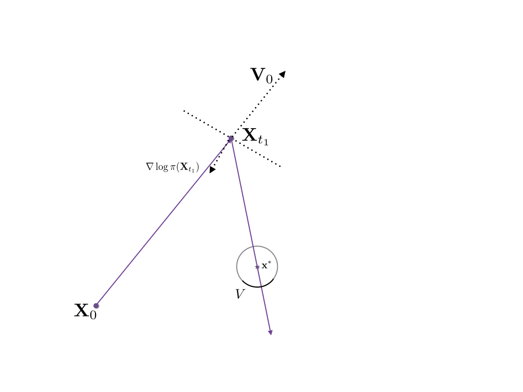
We illustrate Case 1 in Figure 9.

Refer to caption
Figure 9: Case1

Case 2: If

Vol​(⋂t∈[t1−δ1,t1+δ1]𝕊⁡(B⁡(𝕩∗,r1)−𝕩t)​⋂V)=0\text{Vol}\left(\displaystyle{\bigcap_{t\in[t_{1}-\delta_{1},t_{1}+\delta_{1}]}}\mathbb{S}\left(B\left(\mathbb{x}^{*},r_{1}\right)-\mathbb{x}_{t}\right)\bigcap V\right)=0

and

⟨𝕊⁡(𝕩∗−𝕩t1),∇log⁡π​(𝕩∗)⟩<0\langle\mathbb{S}(\mathbb{x}^{*}-\mathbb{x}_{t_{1}}),\nabla\log\pi(\mathbb{x}^{*})\rangle<0

By (i), we have ∀𝕩′,𝕩′′∈B⁡(𝕩∗,r1),∀t∈[t1−δ1,t1+δ1]\forall\mathbb{x}^{\prime},\mathbb{x}^{\prime\prime}\in B(\mathbb{x}^{*},r_{1}),\forall t\in[t_{1}-\delta_{1},t_{1}+\delta_{1}],

⟨𝕩′−(𝕩0+t​𝕧0),∇log⁡π​(𝕩′′)⟩<0.\langle\mathbb{x}^{\prime}-(\mathbb{x}_{0}+t\mathbb{v}_{0}),\nabla\log\pi(\mathbb{x}^{\prime\prime})\rangle<0.

Denote

𝕄1=⋂𝕩∈B(𝕩∗,r1),𝕧∈𝕊(𝕩−𝕩t),t∈[t1−δ1,t1+δ1]S⟂​(𝕩,𝕧)\mathbb{M}_{1}\quad=\bigcap_{\begin{subarray}{c}\mathbb{x}\in B(\mathbb{x}^{*},r_{1}),\mathbb{v}\in\mathbb{S}(\mathbb{x}-\mathbb{x}_{t}),\\ t\in[t_{1}-\delta_{1},t_{1}+\delta_{1}]\end{subarray}}S^{\perp}(\mathbb{x},\mathbb{v})

By decreasing δ1,r1\delta_{1},r_{1}, we can have

Vol​(𝕄1​⋂𝕍)>0\text{Vol}\left(\mathbb{M}_{1}\bigcap\mathbb{V}\right)>0

or

Vol​(𝕄1​⋂𝕍)=0,Vol​(𝕄1​⋂𝕍′)>0, where ​𝕍′=𝕍\text{Vol}\left(\mathbb{M}_{1}\bigcap\mathbb{V}\right)=0,\quad\text{Vol}\left(\mathbb{M}_{1}\bigcap\mathbb{V}^{\prime}\right)>0,\text{ where }\mathbb{V}^{\prime}=\mathbb{V}

Case 2.1: If

Vol​(𝕄1​⋂𝕍)>0\text{Vol}\left(\mathbb{M}_{1}\bigcap\mathbb{V}\right)>0

By selecting r2<r1r_{2}<r_{1}, such that the length of segment of the line across 𝕩t\mathbb{x}_{t} and 𝕩′∈B⁡(𝕩∗,r2)\mathbb{x}^{\prime}\in B(\mathbb{x}^{*},r_{2}) in the ball B⁡(𝕩∗,r1)B(\mathbb{x}^{*},r_{1}) is larger than some positive constant c1c_{1}. Then event occurs on each line across 𝕩t\mathbb{x}_{t} and 𝕩′\mathbb{x}^{\prime} during the segment in the ball B⁡(𝕩∗,r1)B(\mathbb{x}^{*},r_{1}) and the changed velocity traverses 𝕍\mathbb{V} with positive probability which is larger than some positive constant p2p_{2}. As a result, there exists some t>0t>0 such that

Pt​((𝕩0,𝕧0),W)>0P_{t}\left((\mathbb{x}_{0},\mathbb{v}_{0}),W\right)>0

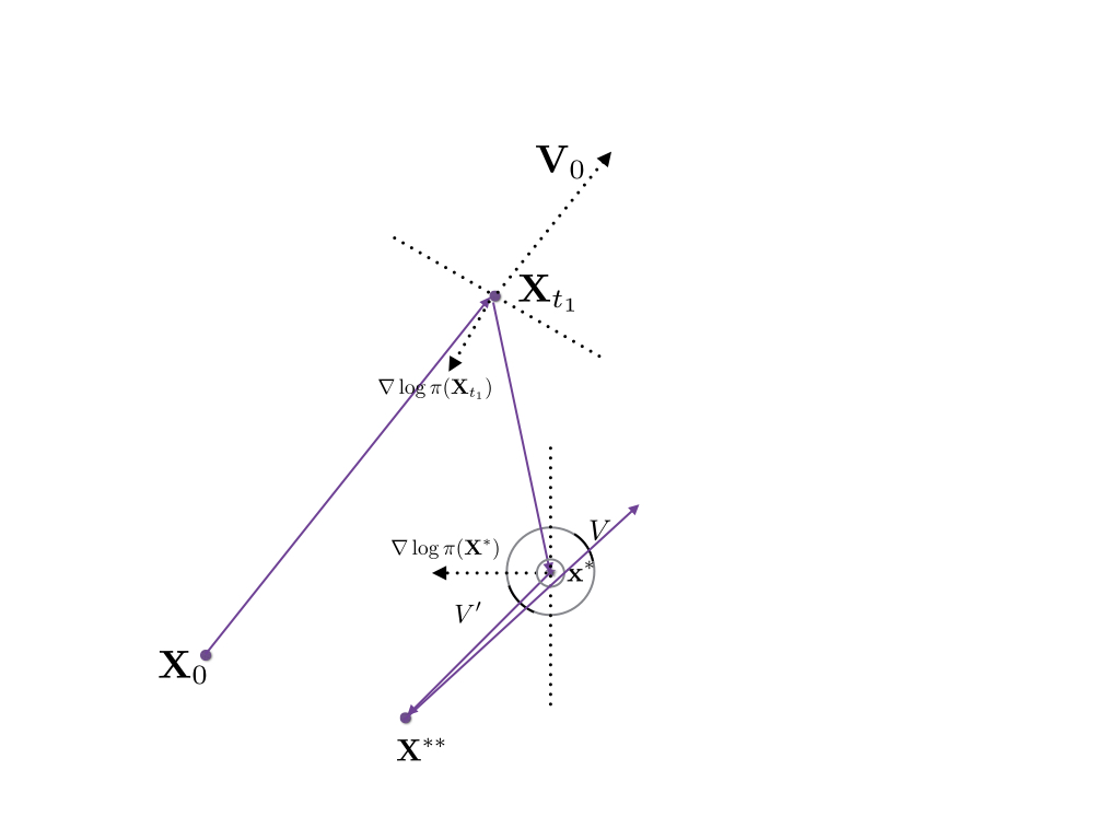
See Figure 10 for illustration.

Refer to caption
Figure 10: Case 2.1

Case 2.2: If

Vol​(𝕄1​⋂𝕍)=0,Vol​(𝕄1​⋂𝕍′)>0, where ​𝕍′=−𝕍\text{Vol}\left(\mathbb{M}_{1}\bigcap\mathbb{V}\right)=0,\quad\text{Vol}\left(\mathbb{M}_{1}\bigcap\mathbb{V}^{\prime}\right)>0,\text{ where }\mathbb{V}^{\prime}=-\mathbb{V}

With the same treatment as that in Case 2.1, there exists 𝕩∗⁣∗\mathbb{x}^{**} such that

𝕊⁡(𝕩∗⁣∗−𝕩∗)∈𝕍′,and ​⟨S⁡(𝕩∗⁣∗−𝕩∗),∇log⁡π​(𝕩∗⁣∗)⟩<0\mathbb{S}(\mathbb{x}^{**}-\mathbb{x}^{*})\in\mathbb{V}^{\prime},\quad\text{and }\langle{S}(\mathbb{x}^{**}-\mathbb{x}^{*}),\nabla\log\pi(\mathbb{x}^{**})\rangle<0

As a result, there exist two positive constants r3>r4r_{3}>r_{4}, such that, if necessary, decreasing r1r_{1} to be small enough,

𝕊⁡(𝕩′′−𝕩′)∈𝕍′, where ​𝕩′∈B⁡(𝕩∗,r1),𝕩′′∈B⁡(𝕩∗⁣∗,r3)\mathbb{S}(\mathbb{x}^{\prime\prime}-\mathbb{x}^{\prime})\in\mathbb{V}^{\prime},\text{ where }\mathbb{x}^{\prime}\in B(\mathbb{x}^{*},r_{1}),\quad\mathbb{x}^{\prime\prime}\in B(\mathbb{x}^{**},r_{3})

and

Vol​(𝕄1​⋂𝕄2​⋂𝕍′)>0,\text{Vol}\left(\mathbb{M}_{1}\bigcap\mathbb{M}_{2}\bigcap\mathbb{V}^{\prime}\right)>0,

where

𝕄2=⋃𝕩′∈B⁡(𝕩∗,r1),𝕩′′∈B⁡(𝕩∗⁣∗,r4)𝕊⁡(𝕩′′−𝕩′).\mathbb{M}_{2}=\bigcup_{\begin{subarray}{c}\mathbb{x}^{\prime}\in B(\mathbb{x}^{*},r_{1}),\\ \mathbb{x}^{\prime\prime}\in B(\mathbb{x}^{**},r_{4})\end{subarray}}\mathbb{S}(\mathbb{x}^{\prime\prime}-\mathbb{x}^{\prime}).

Then, the event, that a particle begins from any point 𝕩′∈B⁡(𝕩∗,r1)\mathbb{x}^{\prime}\in B(\mathbb{x}^{*},r_{1}) with any velocity 𝕧′∈𝕊⁡(B⁡(𝕩∗⁣∗,r4)−𝕩′)\mathbb{v}^{\prime}\in\mathbb{S}(B(\mathbb{x}^{**},r_{4})-\mathbb{x}^{\prime}), changes velocity in the region B⁡(𝕩∗⁣∗,r4)B(\mathbb{x}^{**},r_{4}) to −𝕄2-\mathbb{M}_{2} and passes the area B⁡(𝕩∗,r1)B(\mathbb{x}^{*},r_{1}), occurs with positive probability. As a result, there exists t>0t>0 such that

Pt​((𝕩0,𝕧0),W)>0P_{t}\left((\mathbb{x}_{0},\mathbb{v}_{0}),W\right)>0

See Figure 11 for illustration.

Refer to caption
Figure 11: Case 2.2

Case 3: If

Vol​(⋂t∈[t1−δ1,t1+δ1]𝕊⁡(B⁡(𝕩∗,r1)−𝕩t)​⋂V)=0\text{Vol}\left(\displaystyle{\bigcap_{t\in[t_{1}-\delta_{1},t_{1}+\delta_{1}]}}\mathbb{S}\left(B\left(\mathbb{x}^{*},r_{1}\right)-\mathbb{x}_{t}\right)\bigcap V\right)=0

and

⟨𝕊⁡(𝕩∗−𝕩t1),∇log⁡π​(𝕩∗)⟩>0\langle\mathbb{S}(\mathbb{x}^{*}-\mathbb{x}_{t_{1}}),\nabla\log\pi(\mathbb{x}^{*})\rangle>0

By Assumption 1, there exists 𝕩∗⁣∗\mathbb{x}^{**} on the line which passes 𝕩t1\mathbb{x}_{t_{1}} and 𝕩∗\mathbb{x}^{*}, such that

⟨𝕊⁡(𝕩∗−𝕩t1),∇log⁡π​(𝕩∗⁣∗)⟩<0.\langle\mathbb{S}(\mathbb{x}^{*}-\mathbb{x}_{t_{1}}),\nabla\log\pi(\mathbb{x}^{**})\rangle<0.

Then there exists r5r_{5}, such that, if necessary, decreasing δ1,r1\delta_{1},r_{1} to be small enough,

Vol​(𝕄3​⋂𝕍)>0\text{Vol}\left(\mathbb{M}_{3}\bigcap\mathbb{V}\right)>0

or

Vol​(𝕄3​⋂𝕍)=0​, and Vol​(𝕄3​⋂𝕍′)>0, where ​𝕍′=−𝕍\text{Vol}\left(\mathbb{M}_{3}\bigcap\mathbb{V}\right)=0\text{, and }\text{Vol}\left(\mathbb{M}_{3}\bigcap\mathbb{V}^{\prime}\right)>0,\text{ where }\mathbb{V}^{\prime}=-\mathbb{V}

where

𝕄3=⋂𝕩∈B⁡(𝕩∗,r1),𝕧∈𝕊⁡(𝕩−B⁡(𝕩∗⁣∗,r5))S⟂​(𝕩,𝕧)\mathbb{M}_{3}=\bigcap_{\begin{subarray}{c}\mathbb{x}\in B(\mathbb{x}^{*},r_{1}),\\ \mathbb{v}\in\mathbb{S}(\mathbb{x}-B(\mathbb{x}^{**},r_{5}))\end{subarray}}S^{\perp}(\mathbb{x},\mathbb{v})

Case 3.1: If

Vol​(𝕄3​⋂𝕍)>0\text{Vol}\left(\mathbb{M}_{3}\bigcap\mathbb{V}\right)>0

Then, the event that a particle begins from any point 𝕩t,t∈[t1−δ1,t​1+δ1]\mathbb{x}_{t},t\in[t_{1}-\delta_{1},t1+\delta_{1}] with velocity 𝕧\mathbb{v}, passes the region B⁡(𝕩∗,r1)B(\mathbb{x}^{*},r_{1}), changes velocity in the region B⁡(𝕩∗⁣∗,r5)B(\mathbb{x}^{**},r_{5}) to 𝕧′∈𝕊⁡(B⁡(𝕩∗,r1)−B⁡(𝕩∗⁣∗,r5))\mathbb{v}^{\prime}\in\mathbb{S}(B(\mathbb{x}^{*},r_{1})-B(\mathbb{x}^{**},r_{5})), reaches the area B⁡(𝕩∗,r1)B(\mathbb{x}^{*},r_{1}) and changes velocity to 𝕍\mathbb{V} occurs with positive probability. As a result, we obtain the desired result in this case. See Figure 12 for illustration.

Refer to caption
Figure 12: Case 3.1

Case 3.2: If

Vol​(𝕄3​⋂𝕍)=0​, and Vol​(𝕄3​⋂𝕍′)>0, where ​𝕍′=−𝕍\text{Vol}\left(\mathbb{M}_{3}\bigcap\mathbb{V}\right)=0\text{, and }\text{Vol}\left(\mathbb{M}_{3}\bigcap\mathbb{V}^{\prime}\right)>0,\text{ where }\mathbb{V}^{\prime}=-\mathbb{V}

By the similar treatment of Case 3.1 and Case 2.2, we can get the admired result. We give an illustration of Case 3.2 in Figure 13.
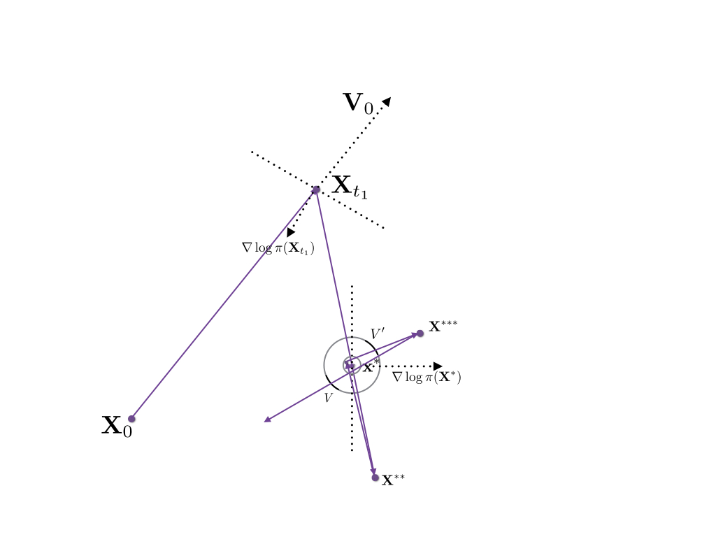
Refer to caption
Figure 13: Case 3.2

∎

With the help of Lemma 1 and Lemma 2, we can prove the ergodicity of GBPS and the way of proof is similar to that of Theorem 1 of [6]

Proof of Theorem 2.

Suppose GBPS is not ergodic, then according to Theorem 7.1 of [11], there exist two measures μ1\mu_{1} and μ2\mu_{2} such that μ1⟂μ2\mu_{1}\perp\mu_{2} and μ1\mu_{1} and μ2\mu_{2} both are the invariant distribution of GBPS. Thus, there is a measurable set A⊂ℝd×Sd−1A\subset\mathbb{R}^{d}\times S_{d-1} such that

μ1​(A)=μ2​(Ac)=0\mu_{1}(A)=\mu_{2}(A^{c})=0

Let A1=A,A2=AcA_{1}=A,A_{2}=A^{c}. By Lemma 2 and Lemma 2.2 of [11], the support of μi\mu_{i} is ℝd×Sd−1\mathbb{R}^{d}\times S_{d-1}. For any open set B⊂ℝd×Sd−1B\subset\mathbb{R}^{d}\times S_{d-1}, μi​(B)>0\mu_{i}(B)>0. As a result, at least one of A1∩BA_{1}\cap B or A2∩BA_{2}\cap B has a positive volume by the measure on ℝd×Sd−1\mathbb{R}^{d}\times S_{d-1} which is induced by Lebesgue measure on ℝd×ℝd\mathbb{R}^{d}\times\mathbb{R}^{d}. Hence, we denote by i∗∈{1,2}i^{*}\in\{1,2\} an index satisfying Vol​(Ai∗∩B)>0\text{Vol}(A_{i^{*}}\cap B)>0. From Lemma 2, we know there exists a zz in the interior in Ai∗∩BA_{i*}\cap B and t>0t>0 such that Pt​(z,Ai∗)>0P_{t}(z,A_{i^{*}})>0. As a result, there exist r0>0r_{0}>0 and δ>0\delta>0 such that Pt​(z′,Ai∗)>δP_{t}(z^{\prime},A_{i^{*}})>\delta for all z′∈B(z,r0)⊂Ai∗∩Bz^{\prime}\in B(z,r_{0})\subset A_{i*}\cap B. Hence,

μi∗​(Ai∗)=∫μi∗​(d​z′′)​Pt​(z′′,Ai∗)≥∫Bμi∗​(d​z′′)​Pt​(z′′,Ai∗)≥∫B∩Ai∗μi∗​(d​z′′)​δ≥δ​μi∗​(B∩Ai∗)>0\begin{split}\mu_{i^{*}}(A_{i^{*}})&=\int\mu_{i^{*}}(dz^{\prime\prime})P_{t}(z^{\prime\prime},A_{i^{*}})\\ &\geq\int_{B}\mu_{i^{*}}(dz^{\prime\prime})P_{t}(z^{\prime\prime},A_{i^{*}})\\ &\geq\int_{B\cap A_{i^{*}}}\mu_{i^{*}}(dz^{\prime\prime})\delta\\ &\geq\delta\mu_{i^{*}}(B\cap A_{i^{*}})>0\end{split}

This contradicts that μi​(Ai)=0\mu_{i}(A_{i})=0 for i∈{1,2}i\in\{1,2\}. As a result, GBPS has as most one invariant measure. By Lemma 1, we complete the proof. ∎

References

  • [1] Bardenet R, Doucet A, Holmes C. On Markov chain Monte Carlo methods for tall data. arXiv preprint arXiv:1505.02827 (2015).
  • [2] Bierkens J, Roberts G. A piecewise deterministic scaling limit of lifted Metropolis–Hastings in the Curie–Weiss model. The Annals of Applied Probability 27.2 (2017): 846-882.
  • [3] Bierkens J. Non-reversible Metropolis-Hastings. Statistics and Computing 26.6 (2016): 1213-1228.
  • [4] Bierkens J, Fearnhead P, Roberts G. The Zig-Zag Process and Super-Efficient Sampling for Bayesian Analysis of Big Data. arXiv preprint arXiv:1607.03188 (2016).
  • [5] Bierkens J, Bouchard-Côté A, Doucet A, et al. Piecewise Deterministic Markov Processes for Scalable Monte Carlo on Restricted Domains. arXiv preprint arXiv:1701.04244 (2017).
  • [6] Bouchard-Côté A, Vollmer S J, Doucet A. The bouncy particle sampler: A non-reversible rejection-free Markov chain Monte Carlo method. Journal of the American Statistical Association (to appear) (2017).
  • [7] Chen T L, Hwang C R. Accelerating reversible Markov chains. Statistics & Probability Letters 83.9 (2013): 1956-1962.
  • [8] Davis M H A. Piecewise-deterministic Markov processes: A general class of non-diffusion stochastic models. Journal of the Royal Statistical Society. Series B (Methodological) (1984): 353-388.
  • [9] Davis M H A. Markov Models & Optimization. Vol. 49. CRC Press, 1993.
  • [10] Fearnhead P, Bierkens J, Pollock M, et al. Piecewise Deterministic Markov Processes for Continuous-Time Monte Carlo. arXiv preprint arXiv:1611.07873 (2016).
  • [11] Hairer M. Convergence of Markov processes. Lecture notes (2010). http://www.hairer.org/notes/Convergence.pdf
  • [12] Hastings W K. Monte Carlo sampling methods using Markov chains and their applications. Biometrika 57.1 (1970): 97-109.
  • [13] Hwang C R, Hwang-Ma S Y, Sheu S J. Accelerating Gaussian diffusions. The Annals of Applied Probability (1993): 897-913.
  • [14] Kingman J F C. Poisson processes. John Wiley & Sons, Ltd, 1993.
  • [15] Lewis P A, Shedler G S. Simulation of nonhomogeneous Poisson processes by thinning. Naval research logistics quarterly 26.3 (1979): 403-413.
  • [16] Metropolis N, Rosenbluth A W, Rosenbluth M N, et al. Equation of state calculations by fast computing machines. The journal of chemical physics 21.6 (1953): 1087-1092.
  • [17] Minsker S, Srivastava S, Lin L, et al. Robust and scalable Bayes via a median of subset posterior measures. arXiv preprint arXiv:1403.2660 (2014).
  • [18] Neiswanger W, Wang C, Xing E. Asymptotically exact, embarrassingly parallel MCMC. arXiv preprint arXiv:1311.4780 (2013).
  • [19] Peters E A J F. Rejection-free Monte Carlo sampling for general potentials. Physical Review E 85.2 (2012): 026703.
  • [20] Quiroz M, Villani M, Kohn R. Speeding up MCMC by efficient data subsampling. arXiv preprint arXiv:1404.4178 (2014).
  • [21] Scott S L, Blocker A W, Bonassi F V, et al. Bayes and big data: The consensus Monte Carlo algorithm. International Journal of Management Science and Engineering Management 11.2 (2016): 78-88.
  • [22] Sun Y, Schmidhuber J, Gomez F J. Improving the asymptotic performance of Markov chain Monte-Carlo by inserting vortices. Advances in Neural Information Processing Systems. (2010). 2235-2243.
  • [23] Wang X, Dunson D B. Parallelizing MCMC via Weierstrass sampler. arXiv preprint arXiv:1312.4605 (2013).