Deep learning-based numerical methods for high-dimensional parabolic partial differential equations and backward stochastic differential equations

Let $T\in(0,\infty)$, $d\in{\mathbb{N}}$, $\xi\in{\mathbb{R}}^{d}$, let $f\colon{\mathbb{R}}\times{\mathbb{R}}^{d}\to{\mathbb{R}}$ and $g\colon{\mathbb{R}}^{d}\to{\mathbb{R}}$ be continuous functions, and let $u=(u(t,x))_{t\in[0,T],x\in{\mathbb{R}}^{d}}\in C^{1,2}([0,T]\times{\mathbb{R}}^{d},{\mathbb{R}})$ satisfy for all $t\in[0,T]$, $x\in{\mathbb{R}}^{d}$ that $u(T,x)=g(x)$ and

A key idea of this work is to reformulate the PDE (PDE) as an appropriate stochastic control problem.

More specifically, let $(\Omega,\mathcal{F},\mathbbm{P})$ be a probability space, let $W\colon[0,T]\times\Omega\to{\mathbb{R}}^{d}$ be a $d$-dimensional standard Brownian motion on $(\Omega,\mathcal{F},\mathbbm{P})$, let $\mathbb{F}=(\mathbb{F}_{t})_{t\in[0,T]}$ be the normal filtration on $(\Omega,\mathcal{F},\mathbbm{P})$ generated by $W$, let $\mathcal{A}$ be the set of all $\mathbb{F}$-adapted ${\mathbb{R}}^{d}$-valued stochastic processes with continuous sample paths, and for every $y\in{\mathbb{R}}$ and every $Z\in\mathcal{A}$ let $Y^{y,Z}\colon[0,T]\times\Omega\to{\mathbb{R}}$ be an $\mathbb{F}$-adapted stochastic process with continuous sample paths which satisfies that for all $t\in[0,T]$ it holds $\mathbbm{P}$-a.s. that

We now view the solution $u\in C^{1,2}([0,T]\times{\mathbb{R}}^{d},{\mathbb{R}})$ of (PDE) and its spatial derivative as the solution of a stochastic control problem associated to (1). More formally, under suitable regularity hypotheses on the nonlinearity $f$ it holds that the pair consisting of $u(0,\xi)\in{\mathbb{R}}$ and $((\nabla_{x}u)(t,\xi+W_{t}))_{t\in[0,T]}\in\mathcal{A}$ is the (up to indistinguishability) unique global minimum of the function

One can also view the stochastic control problem (1)–(2) (with $Z$ being the control) as a model-based reinforcement learning problem. In that analogy, we view $Z$ as the policy and we approximate $Z\in\mathcal{A}$ using feedforward neural networks (see (11) and Section 4 below for further details). The process $u(t,\xi+W_{t})$, $t\in[0,T]$, corresponds to the value function associated to the stochastic control problem and can be computed approximatively by employing the policy $Z$ (see (9) below for details). The connection between the PDE (PDE) and the stochastic control problem (1)–(2) is based on the nonlinear Feynman-Kac formula which links PDEs and BSDEs (see (BSDE) and (3) below).

Let $Y\colon[0,T]\times\Omega\to{\mathbb{R}}$ and $Z\colon[0,T]\times\Omega\to{\mathbb{R}}^{d}$ be $\mathbb{F}$-adapted stochastic processes with continuous sample paths which satisfy that for all $t\in[0,T]$ it holds $\mathbbm{P}$-a.s. that

Under suitable additional regularity assumptions on the nonlinearity $f$ we have that the nonlinear parabolic PDE (PDE) is related to the BSDE (BSDE) in the sense that for all $t\in[0,T]$ it holds $\mathbbm{P}$-a.s. that

(cf., e.g., [25, Section 3] and [27]). The first identity in (3) is sometimes referred to as nonlinear Feynman-Kac formula in the literature.

To derive the deep BSDE solver, we first plug the second identity in (3) into (BSDE) to obtain that for all $t\in[0,T]$ it holds $\mathbbm{P}$-a.s. that

In particular, we obtain that for all $t_{1},t_{2}\in[0,T]$ with $t_{1}\leq t_{2}$ it holds $\mathbbm{P}$-a.s. that

Next we apply a time discretization to (5). More specifically, let $N\in{\mathbb{N}}$ and let $t_{0},t_{1},\dots,t_{N}\in[0,T]$ be real numbers which satisfy

and observe that (5) suggests for $N\in{\mathbb{N}}$ sufficiently large that

In the next step we employ a deep learning approximation for

but not for $u(t_{n},x)\in{\mathbb{R}}$, $x\in{\mathbb{R}}^{d}$, $n\in\{0,1,\dots,N\}$. Approximations for $u(t_{n},x)\in{\mathbb{R}}$, $x\in{\mathbb{R}}^{d}$, $n\in\{0,1,\dots,N\}$, in turn, can be computed recursively by using (7) together with deep learning approximations for (8). More specifically, let $\rho\in{\mathbb{N}}$, let $\mathcal{U}^{\theta}\in{\mathbb{R}}$, $\theta\in{\mathbb{R}}^{\rho}$, be real numbers, let $\mathcal{V}^{\theta}_{n}\colon{\mathbb{R}}^{d}\to{\mathbb{R}}^{d}$, $n\in\{0,1,\dots,N-1\}$, $\theta\in{\mathbb{R}}^{\rho}$, be continuous functions, and let $\mathcal{Y}^{\theta}\colon\{0,1,\dots,N\}\times\Omega\to{\mathbb{R}}$, $\theta\in{\mathbb{R}}^{\rho}$, be stochastic processes which satisfy for all $\theta\in{\mathbb{R}}^{\rho}$, $n\in\{0,1,\dots,N-1\}$ that $\mathcal{Y}^{\theta}_{0}=\mathcal{U}^{\theta}$ and

We think of $\rho\in{\mathbb{N}}$ as the number of parameters in the neural network, for all appropriate $\theta\in{\mathbb{R}}^{\rho}$ we think of $\mathcal{U}^{\theta}\in{\mathbb{R}}$ as suitable approximations

of $u(0,\xi)$, and for all appropriate $\theta\in{\mathbb{R}}^{\rho}$, $x\in{\mathbb{R}}^{d}$, $n\in\{0,1,\dots,N-1\}$ we think of $\mathcal{V}^{\theta}_{n}(x)\in{\mathbb{R}}^{1\times d}$ as suitable approximations

of $(\nabla_{x}u)(t_{n},x)$.

The “appropriate” $\theta\in{\mathbb{R}}^{\rho}$ can be obtained by minimizing the expected loss function through stochastic gradient descent-type algorithms. For the loss function we pick the squared approximation error associated to the terminal condition of the BSDE (BSDE). More precisely, assume that the function ${\mathbb{R}}^{\rho}\ni\theta\mapsto{\mathbbm{E}}\big[|\mathcal{Y}^{\theta}_{N}-g(\mathcal{X}_{N})|^{2}\big]\in[0,\infty]$ has a unique global minimum and let $\Lambda\in{\mathbb{R}}^{\rho}$ be the real vector for which the function

is minimal. Minimizing the function (12) is inspired by the fact that

according to (BSDE) above (cf. (2) above). Under suitable regularity assumptions, we approximate the vector $\Lambda\in{\mathbb{R}}^{\rho}$ through stochastic gradient descent-type approximation methods and thereby we obtain random approximations $\Theta_{0},\Theta_{1},\Theta_{2},\dots\colon\Omega\to{\mathbb{R}}^{\rho}$ of $\Lambda\in{\mathbb{R}}^{\rho_{\vartheta}}$. For sufficiently large $N,\rho,m\in{\mathbb{N}}$ we then employ the random variable $\mathcal{U}^{\Theta_{m}}\colon\Omega\to{\mathbb{R}}$ as a suitable implementable approximation

of $u(0,\xi)$ (cf. (10) above) and for sufficiently large $N,\rho,m\in{\mathbb{N}}$ and all $x\in{\mathbb{R}}^{d}$, $n\in\{0,1,\dots,N-1\}$ we use the random variable $\mathcal{V}^{\Theta_{m}}_{n}(x)\colon\Omega\to{\mathbb{R}}^{1\times d}$ as a suitable implementable approximation

of $(\nabla_{x}u)(t_{n},x)$ (cf. (11) above). In the next section the proposed approximation method is described in more detail.

To simplify the presentation we have restricted us in (PDE), (1), (2), (BSDE) above and Subsection 3.1 below to semilinear heat equations. We refer to Subsection 3.2 and Section 4 below for the general description of the deep BSDE solver.

In this subsection we describe the algorithm proposed in this article in the specific situation where (PDE) is the PDE under consideration, where batch normalization (see Ioffe & Szegedy [21]) is not employed, and where the plain-vanilla stochastic gradient descent approximation method with a constant learning rate $\gamma\in(0,\infty)$ and without mini-batches is the employed stochastic algorithm. The general framework, which includes the setting in this subsection as a special case, can be found in Subsection 3.2 below.

Under suitable further hypotheses (cf. Sections 4 and 5 below), we think in the case of sufficiently large $\rho,N,m\in{\mathbb{N}}$ and sufficiently small $\gamma\in(0,\infty)$ of $\mathcal{U}^{\Theta_{m}}\in{\mathbb{R}}$ as an appropriate approximation

of the solution $u(t,x)\in{\mathbb{R}}$, $(t,x)\in[0,T]\times{\mathbb{R}}^{d}$, of the PDE

for $(t,x)\in[0,T]\times{\mathbb{R}}^{d}$.

The dynamics in (24) associated to the stochastic processes $(\mathcal{X}^{m,j}_{n})_{n\in\{0,1,\dots,N\}}$ for $m,j\in{\mathbb{N}}_{0}$ allows us to incorporate different algorithms for the discretization of the considered forward stochastic differential equation (SDE) into the deep BSDE solver in Subsection 3.2. The dynamics in (29) associated to the stochastic processes $\Xi_{m}$, $m\in{\mathbb{N}}_{0}$, and $\Theta_{m}$, $m\in{\mathbb{N}}_{0}$, allows us to incorporate different stochastic approximation algorithms such as

• •

  stochastic gradient descent with or without mini-batches (see Subsection 5.1 below) as well as

• •

  adaptive moment estimation (Adam) with mini-batches (see Kingma & Jimmy [22] and Subsection 5.2 below) into the deep BSDE solver in Subsection 3.2.

The dynamics in (28) associated to the stochastic process $\mathbb{S}_{m}$, $m\in{\mathbb{N}}_{0}$, allows us to incorporate the standardization procedure in batch normalization (see Ioffe & Szegedy [21] and also Section 4 below) into the deep BSDE solver in Subsection 3.2. In that case we think of $\mathbb{S}_{m}$, $m\in{\mathbb{N}}_{0}$, as approximatively calculated means and standard deviations.

Assume the setting in Subsection 3.2, assume for all $\theta=(\theta_{1},\dots,\theta_{\rho})\in{\mathbb{R}}^{\rho}$ that $k=1$, $\rho=d+1+(N-1)\left(2d(d+10)+(d+10)^{2}+4(d+10)+2d\right)$, $\varrho=2\rho$, $\mathcal{U}^{\theta}=\theta_{1}$, $\Xi_{0}=0$, let $\mu\colon[0,T]\times{\mathbb{R}}^{d}\to{\mathbb{R}}^{d}$ and $\sigma\colon[0,T]\times{\mathbb{R}}^{d}\to{\mathbb{R}}^{d\times d}$ be functions, let $u\colon[0,T]\times{\mathbb{R}}^{d}\to{\mathbb{R}}$ be a continuous and at most polynomially growing function which satisfies for all $(t,x)\in[0,T)\times{\mathbb{R}}^{d}$ that $u|_{[0,T)\times{\mathbb{R}}^{d}}\in C^{1,2}([0,T)\times{\mathbb{R}}^{d},{\mathbb{R}})$, $u(T,x)=g(x)$, and

let $\varepsilon=10^{-8}$, $\mathbb{X}=\frac{9}{10}$, $\mathbb{Y}=\frac{999}{1000}$, $J=64$, $(\gamma_{m})_{m\in{\mathbb{N}}}\subseteq(0,\infty)$, let $\operatorname{Pow}_{r}\colon{\mathbb{R}}^{\rho}\to{\mathbb{R}}^{\rho}$, $r\in(0,\infty)$, be the functions which satisfy for all $r\in(0,\infty)$, $x=(x_{1},\dots,x_{\rho})\in{\mathbb{R}}^{\rho}$ that

and assume for all $m\in{\mathbb{N}}$, $x,y\in{\mathbb{R}}^{\rho}$, $(\varphi_{j})_{j\in{\mathbb{N}}}\in({\mathbb{R}}^{\rho})^{{\mathbb{N}}}$ that

and

(cf. Example 5.2 below and Kingma & Ba [22]).

In this section we test the deep BSDE solver in the case of an $100$-dimensional Allen-Cahn PDE with a cubic nonlinearity (see (35) below).

More specifically, assume the setting in the Subsection 4.1 and assume for all $s,t\in[0,T]$, $x,w\in{\mathbb{R}}^{d}$, $y\in{\mathbb{R}}$, $z\in{\mathbb{R}}^{1\times d}$, $m\in{\mathbb{N}}$ that $\gamma_{m}=5\cdot 10^{-4}$, $d=100$, $T=\frac{3}{10}$, $N=20$, $\mu(t,x)=0$, $\sigma(t,x)w=\sqrt{2}\,w$, $\xi=(0,0,\dots,0)\in{\mathbb{R}}^{d}$, $\Upsilon(s,t,x,w)=x+\sqrt{2}\,w$, $f(t,x,y,z)=y-y^{3}$, and $g(x)=\left[2+\frac{2}{5}\,\|x\|_{{\mathbb{R}}^{d}}^{2}\right]^{-1}$. Note that the solution $u$ of the PDE (30) then satisfies for all $t\in[0,T)$, $x\in{\mathbb{R}}^{d}$ that $u(T,x)=g(x)$ and

In Table 1 we approximatively calculate the mean of $\mathcal{U}^{\Theta_{m}}$, the standard deviation of $\mathcal{U}^{\Theta_{m}}$, the relative $L^{1}$-approximatin error associated to $\mathcal{U}^{\Theta_{m}}$, the standard deviation of the relative $L^{1}$-approximatin error associated to $\mathcal{U}^{\Theta_{m}}$, and the runtime in seconds needed to calculate one realization of $\mathcal{U}^{\Theta_{m}}$ against $m\in\{0,1000,2000,3000,4000\}$ based on $5$ independent realizations ($5$ independent runs) (see also the Python code 1 below). Table 1 also depicts the mean of the loss function associated to $\Theta_{m}$ and the standard deviation of the loss function associated to $\Theta_{m}$ against $m\in\{0,1000,2000,3000,4000\}$ based on $256$ Monte Carlo samples and $5$ independent realizations ($5$ independent runs). In addition, the relative $L^{1}$-approximation error associated to $\mathcal{U}^{\Theta_{m}}$ against $m\in\{1,2,3,\dots,4000\}$ is pictured on the left hand side of Figure 2 based on $5$ independent realizations ($5$ independent runs) and the mean of the loss function associated to $\Theta_{m}$ against $m\in\{1,2,3,\dots,4000\}$ is pictured on the right hand side of Figure 2 based on $256$ Monte Carlo samples and $5$ independent realizations ($5$ independent runs). In the approximative computations of the relative $L^{1}$-approximation errors in Table 1 and Figure 2 the value $u(0,\xi)=u(0,0,\dots,0)$ of the exact solution $u$ of the PDE (35) is replaced by the value $0.052802$ which, in turn, is calculated by means of the Branching diffusion method (see the Matlab code 2 below and see, e.g., [17, 19, 18] for analytical and numerical results for the Branching diffusion method in the literature).

In this subsection we apply the deep BSDE solver in Subsection 3.2 to a Hamilton-Jacobi-Bellman (HJB) equation which admits an explicit solution that can be obtained through the Cole-Hopf transformation (cf., e.g., Chassagneux & Richou [7, Section 4.2] and Debnath [10, Section 8.4]).

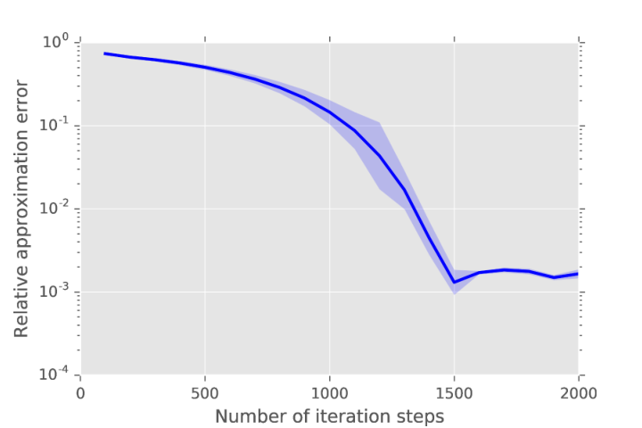
Assume the setting in the Subsection 4.1 and assume for all $s,t\in[0,T]$, $x,w\in{\mathbb{R}}^{d}$, $y\in{\mathbb{R}}$, $z\in{\mathbb{R}}^{1\times d}$, $m\in{\mathbb{N}}$ that $d=100$, $T=1$, $N=20$, $\gamma_{m}=\frac{1}{100}$, $\mu(t,x)=0$, $\sigma(t,x)w=\sqrt{2}\,w$, $\xi=(0,0,\dots,0)\in{\mathbb{R}}^{d}$, $\Upsilon(s,t,x,w)=x+\sqrt{2}\,w$, $f(t,x,y,z)=-\|z\|^{2}_{{\mathbb{R}}^{1\times d}}$, and $g(x)=\ln(\frac{1}{2}\,[1+\|x\|^{2}_{{\mathbb{R}}^{d}}])$. Note that the solution $u$ of the PDE (30) then satisfies for all $t\in[0,T)$, $x\in{\mathbb{R}}^{d}$ that $u(T,x)=g(x)$ and

References

• [1] Bellman, R. Dynamic programming. Princeton Landmarks in Mathematics. Princeton University Press, Princeton, NJ, 2010. Reprint of the 1957 edition, With a new introduction by Stuart Dreyfus.
• [2] Bender, C., and Denk, R. A forward scheme for backward SDEs. Stochastic Processes and their Applications 117, 12 (2007), 1793–1812.
• [3] Bender, C., Schweizer, N., and Zhuo, J. A primal-dual algorithm for BSDEs. arXiv:1310.3694 (2014), 36 pages.
• [4] Bergman, Y. Z. Option pricing with differential interest rates. Review of Financial Studies 8, 2 (1995), 475–500.
• [5] Briand, P., and Labart, C. Simulation of BSDEs by Wiener chaos expansion. Ann. Appl. Probab. 24, 3 (06 2014), 1129–1171.
• [6] Chassagneux, J.-F. Linear multistep schemes for BSDEs. SIAM J. Numer. Anal. 52, 6 (2014), 2815–2836.
• [7] Chassagneux, J.-F., and Richou, A. Numerical simulation of quadratic BSDEs. Ann. Appl. Probab. 26, 1 (2016), 262–304.
• [8] Crisan, D., and Manolarakis, K. Solving backward stochastic differential equations using the cubature method: Application to nonlinear pricing. SIAM Journal on Financial Mathematics 3, 1 (2012), 534–571.
• [9] Darbon, J., and Osher, S. Algorithms for overcoming the curse of dimensionality for certain Hamilton-Jacobi equations arising in control theory and elsewhere. Res. Math. Sci. 3 (2016), Paper No. 19, 26.
• [10] Debnath, L. Nonlinear partial differential equations for scientists and engineers, third ed. Birkhäuser/Springer, New York, 2012.
• [11] E, W., Hutzenthaler, M., Jentzen, A., and Kruse, T. On full history recursive multilevel Picard approximations and numerical approximations for high-dimensional nonlinear parabolic partial differential equations and high-dimensional nonlinear backward stochastic differential equations. arXiv:1607.03295 (2017), 46 pages.
• [12] Gobet, E., Lemor, J.-P., and Warin, X. A regression-based Monte Carlo method to solve backward stochastic differential equations. Ann. Appl. Probab. 15, 3 (2005), 2172–2202.
• [13] Gobet, E., and Turkedjiev, P. Linear regression MDP scheme for discrete backward stochastic differential equations under general conditions. Math. Comp. 85, 299 (2016), 1359–1391.
• [14] Gobet, E., and Turkedjiev, P. Adaptive importance sampling in least-squares Monte Carlo algorithms for backward stochastic differential equations. Stochastic Process. Appl. 127, 4 (2017), 1171–1203.
• [15] Goodfellow, I., Bengio, Y., and Courville, A. Deep Learning. MIT Press, 2016. http://www.deeplearningbook.org.
• [16] Han, J., and E, W. Deep Learning Approximation for Stochastic Control Problems. arXiv:1611.07422 (2016), 9 pages.
• [17] Henry-Labordère, P. Counterparty risk valuation: a marked branching diffusion approach. arXiv:1203.2369 (2012), 17 pages.
• [18] Henry-Labordère, P., Oudjane, N., Tan, X., Touzi, N., and Warin, X. Branching diffusion representation of semilinear PDEs and Monte Carlo approximation. arXiv:1603.01727 (2016), 30 pages.
• [19] Henry-Labordère, P., Tan, X., and Touzi, N. A numerical algorithm for a class of BSDEs via the branching process. Stochastic Process. Appl. 124, 2 (2014), 1112–1140.
• [20] Hinton, G. E., Deng, L., Yu, D., Dahl, G., Mohamed, A., Jaitly, N., Senior, A., Vanhoucke, V., Nguyen, P., Sainath, T., and Kingsbury, B. Deep neural networks for acoustic modeling in speech recognition. Signal Processing Magazine 29 (2012), 82–97.
• [21] Ioffe, S., and Szegedy, C. Batch normalization: accelerating deep network training by reducing internal covariate shift. Proceedings of The 32nd International Conference on Machine Learning (ICML), June 2015.
• [22] Kingma, D., and Ba, J. Adam: a method for stochastic optimization. Proceedings of the International Conference on Learning Representations (ICLR), May 2015.
• [23] Krizhevsky, A., Sutskever, I., and Hinton, G. E. Imagenet classification with deep convolutional neural networks. Advances in Neural Information Processing Systems 25 (2012), 1097–1105.
• [24] LeCun, Y., Bengio, Y., and Hinton, G. Deep learning. Nature 521 (2015), 436–444.
• [25] Pardoux, É., and Peng, S. Backward stochastic differential equations and quasilinear parabolic partial differential equations. In Stochastic partial differential equations and their applications (Charlotte, NC, 1991), vol. 176 of Lecture Notes in Control and Inform. Sci. Springer, Berlin, 1992, pp. 200–217.
• [26] Pardoux, É., and Peng, S. G. Adapted solution of a backward stochastic differential equation. Systems Control Lett. 14, 1 (1990), 55–61.
• [27] Pardoux, E., and Tang, S. Forward-backward stochastic differential equations and quasilinear parabolic PDEs. Probab. Theory Related Fields 114, 2 (1999), 123–150.
• [28] Peng, S. G. Probabilistic interpretation for systems of quasilinear parabolic partial differential equations. Stochastics Stochastics Rep. 37, 1-2 (1991), 61–74.