A note on entanglement edge modes in Chern Simons theory

In the ground state of a continuum QFT, the matrix elements of the (un-normalized) reduced density matrix $\tilde{\rho}_{A}$ can be represented by a path integral with a cut along region $A$

where $A^{\pm}$ refers to the upper and lower edge of the cut. While this representation is adequate for the computing the entanglement entropy via the replica trick, it obscures the factorization of the Hilbert space. What should be done with the degrees of freedom living on the entangling surface $\partial A$, which naively belongs to both region A and B? As noted in recent works [17] [18], the resolution is to remove a small tubular neighborhood of the entangling surface, resulting in a stretched co-dimension 1 space-time boundary. For certain backgrounds and choice of $A$ and $B$, we can choose the angular coordinate $\theta$ around the entangling surface as the Euclidean time coordinate. In such cases we can write the trace of $\tilde{\rho}_{A}$ as a path ordered exponential in $\theta$

where $K_{A}$ generates translations in $\theta$. In a topological theory $K_{A}$ is a conserved charge independent of $\theta$ so this reduces to $Z_{A}=e^{-2\pi K_{A}}$, which can be interpreted as a thermal partition function at temperature $2\pi$. The Modular Hamiltonian $\mathcal{H}_{A}=2\pi K_{A}$ is thus a local Hamiltonian on $A$, and the entanglement entropy is identified with the thermal entropy of $Z_{A}$. Due to the presence of the stretched entangling surface, $\mathcal{H}_{A}$ will in general have boundary terms describing the edge degrees of freedom. In the next section we will derive the Modular Hamiltonian for a disk in Chern Simons gauge theory and show how these edge modes are entangled.

The Chern Simons Hilbert space on a closed, compact Riemann surface $\Sigma$ is equivalent to the space of conformal blocks of a chiral WZW model on $\Sigma$ [19]. On the other hand, when we make a spatial decomposition

the Chern Simons Hilbert spaces on $A$ and $B$ are those of the edge chiral WZW model on $\partial A$ and $\partial B$. By preparing states in $H_{\Sigma}$ with the Euclidean path integral we will provide an explicit formula for their embedding into the extended Hilbert space

where $H_{A}$ and $H_{B}$ are the chiral and anti chiral Hilbert spaces living entirely on the edge.

The simplest setting in which we can realize (11) is for the vacuum state on $\Sigma=S^{2}$ and a disk-like region $A$. This state $\ket{\psi}$ is prepared by the Euclidean path integral on a solid ball $B^{3}$ with the spatial $S^{2}$ as its boundary. Just as we did for the reduced density matrix, we will regulate this geometry by removing a semi-tubular neighborhood of the circle $\partial A$ of radial size $\epsilon$. We can then slice the path integral using an angular time coordinate $\theta$ that encircles the entangling surface. The advantage of this time slicing is that the (un-normalized) wave functional $\braket{\phi_{A},\phi_{B}|\psi}$ can be viewed as an amplitude between states living on $A$ and $B$ [20]:

where $K_{A}$ generates rotations around the entangling surface and $\mathcal{J}$ is an anti-linear operator that implements a CPT transformation.

The parity transformation is needed because the $\pi$ rotation on the RHS of (12) requires that $\ket{\phi_{A}}$ and $\mathcal{J}\ket{\phi_{A}}$ have opposite orientations, the C transformation accounts for the bra $\rightarrow$ ket mapping $\bra{\phi_{A}}\rightarrow\ket{\phi_{A}}$, and the $T$ transformation accounts for the fact that $\theta$ and $t$ are oppositely oriented on region $B$ [21].

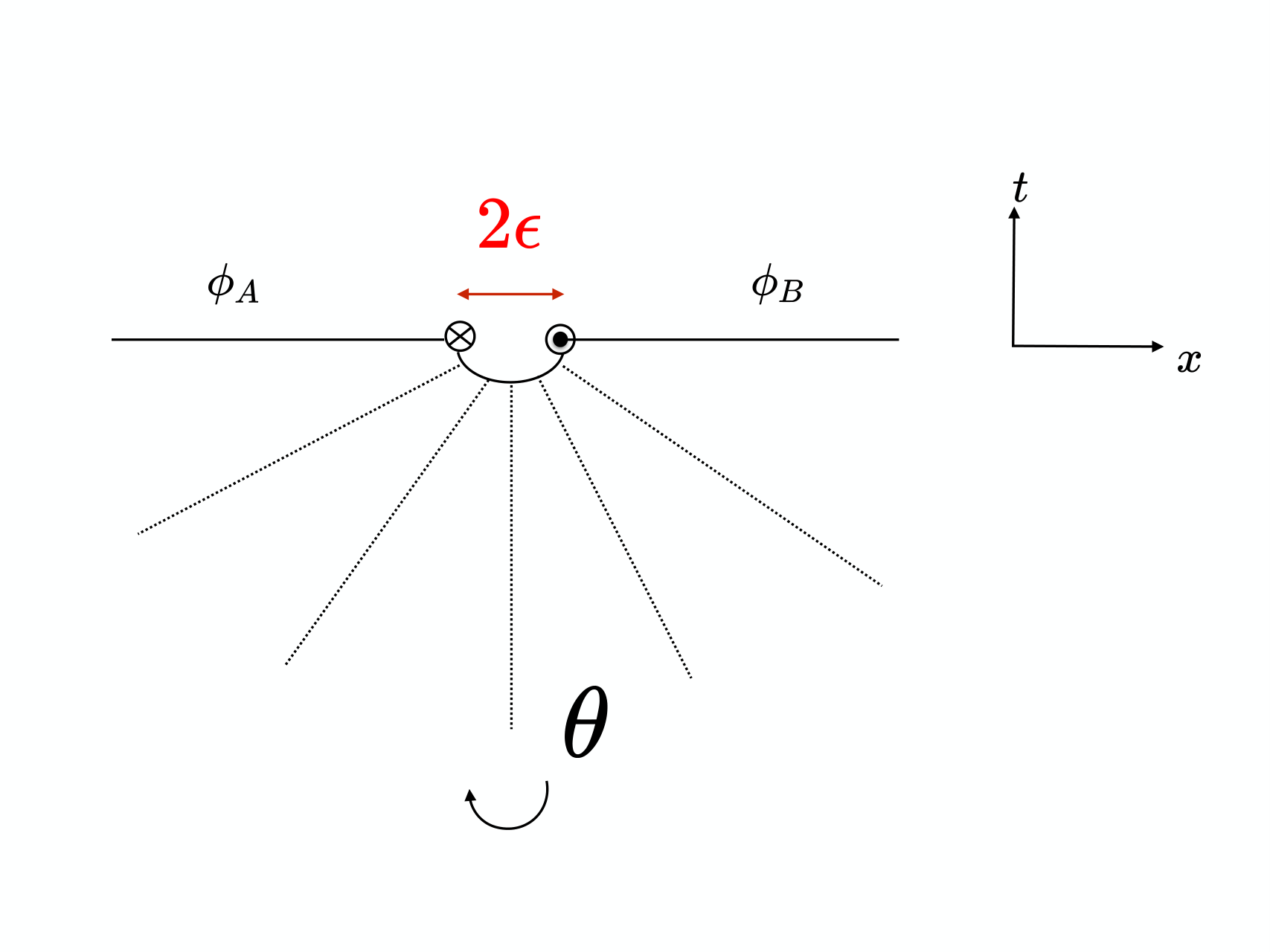
The operator $K_{A}$ evaluated at $\theta=0$ generates infinitesimal translations in the $t=x^{0}$ direction and is therefore the integral of the physical energy density $T_{00}$ weighted by a function $f(x)$

In the bulk of $A$, $T_{00}$ is zero. As noted earlier, quantizing Chern Simons theory on $A$ leads to a chiral CFT Hilbert space living on the edge. Thus the energy density is a delta function supported on the boundary $\partial A$, which we take to be the “stretched” surface at distance $\epsilon$ away from the entangling surface.

In a neighborhood of the entangling surface we can choose local coordinates $(r,\theta,y^{i})$, with $r$ a radial coordinate away from the entangling surface and $y^{i}$ parametrizing the surface itself. In this neighborhood, $f(x)\sim r$, so that $K_{A}$ takes the form of a (Euclidean) Rindler Hamiltonian. Due to the delta function in (15) we can relate $K_{A}$ to the Hamiltonian of the chiral edge CFT:

For a circular boundary of length $l$ we can express the Hamiltonian in terms of the right moving Virasoro generator $L_{0}$ and the central charge $c$.

Expanding in a complete set of eigenstates of the Modular Hamiltonian in $A$ and $B$ in (12) and using the anti linearity of $\mathcal{J}$ leads to a representation of $\ket{\Psi}$ as a thermofield double state of the boundary CFT’s.

where we used the anti-linearity of $\mathcal{J}$ in the second line and denoted $\ket{\bar{m}_{A}}=\mathcal{J}\ket{m_{B}}$ in the third line [20]. Adding the normalization factor $Z_{A}$, we thus arrive at the extended hilbert space factorization of the “bulk” state $\ket{\psi}$

where $\ket{n_{B}}$ and $\ket{\bar{n}_{A}}$ are CPT conjugate states, corresponding to the right and left moving energy eigenstates of the edge CFT’s, and $E_{n}$ are the right moving eigenvalues. Thus the bulk entanglement between the two disks are given entirely by the left-right entanglement of the edge CFT, as noted previously in [12], [13].

Equation (19) gives an explicit embedding of the state $\ket{\psi}$ into the extended Hilbert space. The state $\ket{I}=\sum_{n}\ket{\bar{n}_{A}}\otimes\ket{n_{B}}$ is an Ishibashi state [22], which solves the conformally invariant boundary condition

The thermo-field double state in (19) is a regularized Ishibashi state that has been rendered normalizable by evolving it with the CFT Hamiltonian for a small time $\epsilon$. We will see the relevance of (20) in the next section.

From (19) we can identify the $H_{\text{CFT}}$ with the modular Hamiltonian. The reduced density matrix on $A$ is just the thermal density matrix at inverse temperature $2\pi\epsilon$:

The normalization $Z_{A}$ is given by the finite temperature partition function of CFT.

Thus we see the edge modes partition function arise directly via the regularization of the entangling surface. For generic regions $A$ and $B$, we may not be able to find a globally well defined coordinate $\theta$ on the three manifold $M$ that evolves one region onto the other. ¹¹ 1 However, after regularizing, we can always find such a coordinate locally near the entangling surface that evolves $\partial A$ into $\partial B$. Since $T_{00}$ vanishes in the bulk, this may be sufficient to generalize the path integral argument to other regions. In the next section we will provide another argument for the extended Hilbert space factorization , based on the requirements of gauge invariance in the presence of the entangling surface, which generalizes more readily to an arbitrary region A.

To begin, we recall how imposing gauge invariance in the presence of a boundary leads to new boundary degrees of freedom that transform under a boundary symmetry group. The Chern Simons action

on a manifold $M$ is not gauge invariant when $\partial M$ has a boundary. This is because the on-shell variation gives a boundary term:

One way to restore gauge invariance is to restrict gauge transformations to be trivial on the boundary. This means that the would-be pure gauge degrees of freedom living on $\partial M$ are promoted to dynamical degrees of freedom. These edge modes transform non trivially under the boundary gauge group, which is promoted to a physical symmetry.

To be explicit, consider the the manifold $M=D\times S^{1}$ with $D$ a disk. We have compactified the time dimension, which we will interpret as the angular direction $\theta$ around the entangling surface. Quantization of Chern Simons on a disk was worked out in [24],[19]. Following [24], we choose the boundary condition $A_{0}=0$ to set the boundary term (24) to zero, thus obtaining a well defined variational principle for the bulk equations of motion. The gauss law constraint $\frac{\delta S}{\delta A_{0}}=0$ restricts to flat connections on $D$, which are of the form.

where $\tilde{d}$ is the spatial exterior derivative on $D$ , and $U\in G$ is an element of the gauge group $G$. Note that this is only pure gauge in the bulk, since gauge transformations are required to be trivial on the boundary. Inserting (25) back into the Chern Simons action gives the chiral WZW action

This action only depends on the boundary values²² 2 The second term involves an integration over the bulk but for integer $k$ different bulk extensions of $U$ differ by integer multiples of $2\pi i$ , therefore giving the same exponential weighting in the path integral. of $U$. Gauge fixing and dividing by the volume of the gauge group in the bulk then leads to a boundary theory with the path integral

where $U:\partial D\times R\rightarrow G$. Thus Chern Simons theory on a disk is equivalent to a chiral WZW model living on the edge.

As alluded to earlier, the boundary symmetry group consist of the gauge transformation restricted to the boundary. In order to preserve the boundary condition $A_{0}=0$ these are also required to be time independent. Thus the boundary symmetry group is the loop group $LG$, whose elements

are maps from the boundary circle to the gauge group. Explicitly, the loop group elements acts on the WZW model via

The Hilbert space thus furnishes a representation of the loop group, or equivalently the current algebra of the gauge group G. The currents generating this algebra are just the boundary values of the gauge field

where $z$ is a holomorphic coordinate on the boundary spacetime, and $a$ is a group index.

For example, in the abelian case with gauge group $G=U(1)$, $U=e^{i\theta}$ and the WZW model reduces to a chiral, compact boson $\theta$ with radius $\sim\frac{1}{k}$. The modes of the boson current $J(z)=\partial_{z}\theta$ satisfy the infinite dimensional current algebra at level k:

Up to the $k$ dependent normalization, this is just an infinite set of harmonic oscillators, with the $n>0$ currents acting as annihilation and $n<0$ acting as creation operators. A representation of this algebra is obtained by applying $J_{-n}$ to the highest weight state $\ket{0}$ which is annihilated by $J_{n}$ for $n>0$. When $G$ is non-abelian, the level $k$ current algebra is

where $f^{abc}$ are the structure constants of $G$. In this case the zero modes $J_{0}^{a}$ generate the finite dimensional Lie algebra of $G$ and the highest weight states $\ket{r}$ transforms in an irreducible representation $r$ of G. Only a subset of representations $r$ of $G$ admit the infinite dimensional generalization (32), and each corresponds to a primary field. For example, for $G=SU(2)$, the ground states transform in the usual $2r+1$ dimensional representations with basis elements:

and the Hilbert space is created from the highest weight state $\ket{r,r}$ via the ladder operators $J^{a}_{-n}$ and $J_{0}^{1}-iJ^{2}_{0}$. The allowed “integrable” representations corresponds to half-integers $r$ satsifying $0\leq r<k$. From the point of view of the bulk Chern Simons theory, states in different representations are prepared by a path integral Wilson line inserted inside $D\times R$ in the representation $r$[19] [24].

Now let us return to the original question of how to glue together two Hilbert spaces $H_{A}$ and $H_{B}$. We take $A=D$ and $B=\bar{D}$ to be two oppositely oriented disks, which we wish to glue into a sphere $S^{2}=D\cup\bar{D}$. $H_{A}$ and $H_{B}$ provides a representation of the chiral currents $J^{a}(z)$ anti-chiral currents $\bar{J}^{a}(\bar{z})$ respectively. Since the total Hilbert space $H_{S^{2}}$ is gauge invariant, whereas the tensor product $H_{A}\otimes H_{B}$ transforms non-trivially under $G$, we must restrict to a gauge invariant subspace. This subspace is denoted by the entangling product

defined as a quotient of the tensor product $H_{A}\otimes H_{B}$ by the simultaneous action of the boundary symmetry group on $\partial A$ and $\partial B$. In other words, a state $\ket{\Psi}\in H_{A}\otimes_{G}H_{B}$ is a singlet under the diagonal action of the loop group on the two edges of opposite chirality. Such a state is invariant under the current algebra and satisfies the constraint [22]

For each representation of the current algebra corresponding to a primary with weight $r$, there is a solution to this equation given by the an Ishibashi state [22]

where $\ket{r,n}_{B}$ is a basis in the $r$ representation of the chiral current algebra, and the CPT conjugate $\ket{r,\bar{n}}_{A}=\mathcal{J}\ket{r,n}_{B}$ is the anti chiral counterpart. We can see that this is a solution by taking an arbitrary state $\ket{\bar{a}}\ket{b}$ and computing the the overlap

Here we have made use of the identities $\braket{\mathcal{J}a|\mathcal{J}b}=\braket{a|b}^{*}$ and $\braket{a|\mathcal{J}b}=\braket{\mathcal{J}^{\dagger}a|b}^{*}$ due to the anti-linearity of $\mathcal{J}$. For the vacuum representation, normalizing the state (36) by applying the CFT evolution operator gives the same result obtained in the previous section by path integral methods. More generally, the choice of representation is determined by the bulk state $\ket{\Psi_{r}}$, which is prepared by the path integral on a solid ball $B^{3}$ with a Wilson line in the $r$ representation inserted. The endpoints of the Wilson line corresponding to anyonic charges $r$ and $\bar{r}$ are inserted inside $D$ and $\bar{D}$ of the bounding sphere $S^{2}=\partial B^{3}$. Accounting for the normalization, such a state factorizes as

The constraint (35), also implies the conformally invariant boundary condition (20). This is because the the generators of the current algebra is directly related to the Virasoro generators via the Sugawara construction [25]:

References

- (1) W. Donnelly and L. Freidel, “Local subsystems in gauge theory and gravity,” arXiv:1601.04744 [hep-th].
- (2) M. Van Raamsdonk, “Building up spacetime with quantum entanglement,” Gen. Rel. Grav. 42 (2010) 2323–2329, arXiv:1005.3035 [hep-th]. [Int. J. Mod. Phys.D19,2429(2010)].
- (3) B. Swingle and M. Van Raamsdonk, “Universality of Gravity from Entanglement,” arXiv:1405.2933 [hep-th].
- (4) T. Faulkner, M. Guica, T. Hartman, R. C. Myers, and M. Van Raamsdonk, “Gravitation from Entanglement in Holographic CFTs,” JHEP 03 (2014) 051, arXiv:1312.7856 [hep-th].
- (5) H. Li and F. Haldane, “Entanglement Spectrum as a Generalization of Entanglement Entropy: Identification of Topological Order in Non-Abelian Fractional Quantum Hall Effect States,” Phys. Rev. Lett. 101 no. 1, (2008) 010504.
- (6) W. Donnelly, “Entanglement entropy and nonabelian gauge symmetry,” Class. Quant. Grav. 31 no. 21, (2014) 214003, arXiv:1406.7304 [hep-th].
- (7) W. Donnelly, “Decomposition of entanglement entropy in lattice gauge theory,” Phys.Rev. D85 (2012) 085004, arXiv:1109.0036 [hep-th].
- (8) P. V. Buividovich and M. I. Polikarpov, “Entanglement entropy in lattice gauge theories,” PoS CONFINEMENT8 (2008) 039, arXiv:0811.3824 [hep-lat]. [J. Phys.A42,304005(2009)].
- (9) W. Donnelly and A. C. Wall, “Entanglement entropy of electromagnetic edge modes,” Phys. Rev. Lett. 114 no. 11, (2015) 111603, arXiv:1412.1895 [hep-th].
- (10) W. Donnelly and A. C. Wall, “Geometric entropy and edge modes of the electromagnetic field,” arXiv:1506.05792 [hep-th].
- (11) B. Swingle and T. Senthil, “A Geometric proof of the equality between entanglement and edge spectra,” Phys. Rev. B86 (2012) 045117, arXiv:1109.1283 [cond-mat.str-el].
- (12) X.-L. Qi, H. Katsura, and A. W. Ludwig, “General relationship between the entanglement spectrum and the edge state spectrum of topological quantum states,” Physical review letters 108 no. 19, (2012) 196402.
- (13) D. Das and S. Datta, “Universal features of left-right entanglement entropy,” Phys. Rev. Lett. 115 no. 13, (2015) 131602, arXiv:1504.02475 [hep-th].
- (14) X. Wen, S. Matsuura, and S. Ryu, “Edge theory approach to topological entanglement entropy, mutual information and entanglement negativity in Chern-Simons theories,” Phys. Rev. B93 no. 24, (2016) 245140, arXiv:1603.08534 [cond-mat.mes-hall].
- (15) W. G. Unruh and N. Weiss, “Acceleration Radiation in Interacting Field Theories,” Phys. Rev. D29 (1984) 1656.
- (16) J. R. Fliss, X. Wen, O. Parrikar, C.-T. Hsieh, B. Han, T. L. Hughes, and R. G. Leigh, “Interface Contributions to Topological Entanglement in Abelian Chern-Simons Theory,” arXiv:1705.09611 [cond-mat.str-el].
- (17) J. Cardy and E. Tonni, “Entanglement hamiltonians in two-dimensional conformal field theory,” J. Stat. Mech. 1612 no. 12, (2016) 123103, arXiv:1608.01283 [cond-mat.stat-mech].
- (18) W. Donnelly and G. Wong, “Entanglement branes in a two-dimensional string theory,” arXiv:1610.01719 [hep-th].
- (19) E. Witten, “Quantum Field Theory and the Jones Polynomial,” Commun. Math. Phys. 121 (1989) 351–399.
- (20) T. Jacobson, “Black holes and Hawking radiation in spacetime and its analogues,” Lect. Notes Phys. 870 (2013) 1–29, arXiv:1212.6821 [gr-qc].
- (21) T. Jacobson, “Black hole thermodynamics and the space-time discontinuum,” in Osgood Hill Conference: Conceptual Problems of Quantum Gravity Andover, Massachusetts, May 15-19, 1988, pp. 597–599. 1988.
- (22) N. Ishibashi, “The Boundary and Crosscap States in Conformal Field Theories,” Mod. Phys. Lett. A4 (1989) 251.
- (23) M. Geiller, “Edge modes and corner ambiguities in 3d Chern-Simons theory and gravity,” arXiv:1703.04748 [gr-qc].
- (24) S. Elitzur, G. W. Moore, A. Schwimmer, and N. Seiberg, “Remarks on the Canonical Quantization of the Chern-Simons-Witten Theory,” Nucl. Phys. B326 (1989) 108–134.
- (25) P. H. Ginsparg, “APPLIED CONFORMAL FIELD THEORY,” in Les Houches Summer School in Theoretical Physics: Fields, Strings, Critical Phenomena Les Houches, France, June 28-August 5, 1988, pp. 1–168. 1988. arXiv:hep-th/9108028 [hep-th]. http://inspirehep.net/record/265020/files/arXiv:hep-th_9108028.pdf.
- (26) A. Lewkowycz and J. Maldacena, “Exact results for the entanglement entropy and the energy radiated by a quark,” JHEP 05 (2014) 025, arXiv:1312.5682 [hep-th].
- (27) L. Susskind and J. Uglum, “Black hole entropy in canonical quantum gravity and superstring theory,” Phys. Rev. D50 (1994) 2700–2711, arXiv:hep-th/9401070 [hep-th].
- (28) E. Witten, “Chern-Simons gauge theory as a string theory,” Prog. Math. 133 (1995) 637–678, arXiv:hep-th/9207094 [hep-th].
- (29) R. Gopakumar and C. Vafa, “On the gauge theory / geometry correspondence,” Adv. Theor. Math. Phys. 3 (1999) 1415–1443, arXiv:hep-th/9811131 [hep-th].