1Introduction

Discrepancies in simultaneous explanation of Flavor Anomalies and IceCube PeV Events using Leptoquarks

Bhavesh Chauhan^a,b,#, Bharti Kindra^a,b,⋆, Ashish Narang^a,b,†

$\hskip 9.24994pt{}^{a}$ Physical Research Laboratory, Ahmedabad, India.
$\hskip 9.24994pt{}^{b}$ Indian Institute of Technology, Gandhinagar, India.
$\hskip 9.24994pt{}^{\#}$ bhavesh@prl.res.in $\hskip 9.24994pt{}^{\star}$ bharti@prl.res.in $\hskip 9.24994pt{}^{\dagger}$ ashish@prl.res.in

Abstract: Leptoquarks have been suggested to solve a variety of discrepancies between the expected and observed phenomenon. In this paper, we show that the scalar doublet Leptoquark with Hypercharge 7/6 can simultaneously explain the recent measurement of $R_{K}$ , $R_{K^{*}}$ , the excess in anomalous magnetic moment of muon, and the observed excess in IceCube HESE data. For appropriate choice of couplings, the flavor anomalies are generated at one-loop level and IceCube data is explained via resonant production of the Leptoquark. Several constraints from LHC searches are imposed on the model parameter space.

Keywords: Leptoquarks, IceCube, $R_{K}$ , $R_{K^{*}}$ , $\left(g-2\right)_{\mu}$ , LHC, Monojet

1 Introduction

Leptoquarks are solution to the problem of matter unification which appear naturally in many theories beyond the Standard Model (SM). For example, scalar quarks in R-Parity Violating Supersymmetry (RPV) have Leptoquark like Yukawa couplings [1] whereas vector Leptoquarks arise in Grand Unification Theories (GUT) based on $SU(5)$ and $SO(10)$ [2, 3, 4]. The unique feature of Leptoquarks is that they couple simultaneously to Standard Model (SM) quarks and leptons, thus providing ample testing grounds and applications to variety of discrepancies between theory and experiments.

The latest measurement of $R_{K^{*}}$ and $R_{K}$ by LHCb, has pointed towards $\approx 2.5\sigma$ deviation from the standard model [5, 6]. These are clear hints of Lepton Flavor Universality (LFU) violation which can be explained in a wide variety of frameworks including, but not limited to, Leptoquarks [7, 8, 9, 10, 11, 12], RPV [13, 14, 15, 16], E6 [17], flavor violating Z^′ [18, 19, 20, 21, 22, 23, 24, 25, 26, 27, 28, 29, 30] etc. In the past, Leptoquarks have been used to explain the anomalous magnetic moment of muon [31, 32, 33, 34, 35, 36], flavor anomalies [7, 8, 9, 10, 11, 12], and IceCube PeV events [37, 38, 39, 40, 41, 42, 43] independently. However, simultaneous explanation of all the three observations has not been possible due to the different range of Leptoquark masses required to solve the individual problems. In this work, we show that a scalar Leptoquark of mass close to $1$ TeV can explain the aforementioned discrepancies. However, such an explanation would be extremely unfavoured by LHC data. While the particular results are model dependent, one can make a qualitative predictions about a more general model.

In Section 2 we describe the model of Leptoquark and motivate the texture of the coupling matrices that has been used in this paper. In Section 3 we explain the excess in $\left(g-2\right)_{\mu}$ using this model. In Section 4 we explain the recent measurement of $R_{K}$ and $R_{K^{*}}$ within our framework followed by the explanation for IceCube High Energy Starting Events (HESE) in Section 5. In Section 6 we discuss the results of this analysis and obtain the parameter space for simultaneous explanation. In the next section, we do the LHC analysis for the benchmark point and obtain the constraints. In the end, we conclude with some model-dependent and model-independent statements.

2 Model Description

In this paper, we consider the scalar Leptoquark $\Delta=\left(\mathbf{3,~2,}~7/6\right)$ whose interactions with the SM fields is given as [44],

\mathcal{L}_{\Delta}\ni-(y_{L})_{ij}\bar{u}^{i}_{R}\mathbf{\Delta}_{a}\varepsilon^{ab}(L_{L})_{b}^{j}+(y_{R})_{ij}\bar{Q}_{L}^{i~a}\mathbf{\Delta}_{a}\mathit{l_{R}}^{j}+\text{h.c.}

(1)

where $y_{L(R)}$ are the Yukawa-like couplings of the Leptoquark. For simplicity, we have assumed the couplings to be real. We have not shown the kinetic and Higgs interactions for brevity, however they are relevant for the discussion that follows. We refer the reader to reference [44] for a comprehensive analysis. We can rewrite (1) in terms of the mass eigenstates $\Delta^{5/3}$ and $\Delta^{2/3}$ , where the superscript denotes electric charge. In terms of these states, the Lagrangian (1) is written as,

	$\displaystyle\mathcal{L}_{\Delta}\ni$	$\displaystyle(Vy_{R})_{ij}\bar{u}_{i}P_{R}l_{j}\Delta^{5/3}-(y_{L})_{ij}\bar{u}_{i}P_{L}l_{j}\Delta^{5/3}$		(2)
		$\displaystyle+(y_{R})_{ij}\bar{d}_{i}P_{R}l_{j}\Delta^{2/3}+(y_{L}U)_{ij}\bar{u}_{i}P_{L}\nu_{j}\Delta^{2/3}+\text{\emph{h.c}.}$		(3)

where V and U are the CKM and PMNS matrices respectively. In common literature [44], this model is also known as $\mathbf{R_{2}}$ .

The observed negligible branching ratios of the flavor violating decays of leptons (for example, $\tau\rightarrow\mu\gamma$ and $\mu\rightarrow e\gamma$ ) put stringent constraints on the inter-generation couplings of the Leptoquark. For all practical purposes, this implies that

y_{L(R)}^{qe}=y_{L(R)}^{q\tau}=0\quad\forall q.

(4)

It has been argued in previous works that the this Leptoquark model results in $R_{K}$ $\approx 1$ , and $R_{K^{*}}$ $\approx 1$ because of the tree level contribution to $b\rightarrow s\mu\mu$ [10]. This clearly contradicts the recent measurements by LHCb. It was pointed out in [9] that, if one assumes

y_{R}^{s\mu}=0\quad\text{or}\quad y_{R}^{b\mu}=0,

(5)

then the tree level contribution is negligible and the leading contribution of comes from a one-loop process. It will be shown in Section 4 that this results in $R_{K}$ $<1$ , and $R_{K^{*}}$ $<1$ which is in agreement with the latest experiments. We chose the former solution as it is also favoured by $\left(g-2\right)_{\mu}$ . As mentioned in [9], non-zero $y_{L}^{c\mu}$ results in tree level contribution to $b\rightarrow cl\bar{\nu_{l}}$ which contradicts the observed $R(D)$ and $R(D^{\star})$ . Hence, we also assume that

y_{L}^{c\mu}=0.

(6)

In order to avoid undesired contribution to other rare decays of the B meson, such as $b\rightarrow d\mathit{l^{+}l^{-}}$ , we assume that

y_{R}^{d\mu}\approx 0.

(7)

With these constraints, the coupling matrices are,

\quad y_{L}=\begin{pmatrix}0&y_{L}^{u\mu}&0\\ 0&0&0\\ 0&y_{L}^{t\mu}&0\end{pmatrix}\ ,\quad y_{R}=\begin{pmatrix}0&0&0\\ 0&0&0\\ 0&y_{R}^{b\mu}&0\end{pmatrix}.

(8)

For brevity, we will use $y_{L}^{u\mu}=\lambda_{1},~y_{L}^{t\mu}=\lambda_{2},\text{and}~y_{R}^{b\mu}=\lambda_{3}$ for the remainder of this paper. We will also use $M_{1}$ ( $M_{2}$ ) to denote the mass of $\Delta^{5/3}$ ( $\Delta^{2/3}$ ).

In subsequent sections, it will be pointed out that the LHC constraints limit $M_{1}\geq 1100$ GeV. For our analysis, we take the lower limit and generate constraints on the remaining parameters. If future searches increase the lower limit considerably, the expressions will change accordingly. Having said that, there are only four free parameters in our model

\{M_{2},\lambda_{1},\lambda_{2},\lambda_{3}\}.

(9)

In the subsequent sections, we investigate various constraints on the model parameters coming from $\left(g-2\right)_{\mu}$ , flavor anomalies, IceCube data, and LHC.

3 $\mathbf{\left(g-2\right)_{\mu}}$

The experimentally measured value of the anomalous magnetic moment of muon is slightly larger than the prediction from the Standard Model. This discrepancy has been attributed to a variety of new physics scenarios [45, 31, 32, 33, 46]. At present, the difference is [47],

\delta a_{\mu}=a_{\mu}^{EXP}-a_{\mu}^{SM}=(2.8\pm 0.9)\times 10^{-9}.

(10)

In this model, both of the mass eigenstates contribute to $\left(g-2\right)_{\mu}$ and one can estimate the contribution using expressions given in [44]. Keeping $M_{1}=1100$ GeV, the leptoquark contribution to $\left(g-2\right)_{\mu}$ is given as,

	$\displaystyle a_{\mu}^{\Delta}$	$\displaystyle=1.34\times 10^{-6}~\lambda_{2}\lambda_{3}-\frac{10^{-9}}{(M_{2}/\text{GeV})^{2}}\left(6.11\lambda_{1}^{2}+5.53\lambda_{2}^{2}-9.4\times 10^{4}\lambda_{2}\lambda_{3}+5.53\lambda_{3}^{2}\right)+...$		(11)
		$\displaystyle\approx 1.34\times 10^{-6}~\lambda_{2}\lambda_{3}-10^{-11}\left(8.65~\lambda_{1}^{2}+7.83~\lambda_{2}^{2}+7.83~\lambda_{3}^{2}\right)+\mathcal{O}(10^{-13})$		(12)

where the approximation is obtained using the benchmark point $M_{2}=1000$ GeV. From the above expressions one can see that the leading contribution does not depend on $M_{2}$ . It is also clear that the product $\lambda_{2}\lambda_{3}\approx 10^{-3}$ gives the correct estimate for $\left(g-2\right)_{\mu}$ . In Section 6 we use $a_{\mu}^{\Delta}=\delta a_{\mu}$ to constrain the parameter space of the model.

4 Flavor Anomalies

In the last two decades, loop-induced $b\rightarrow s$ transitions have been playing an active role in understanding the physics beyond the Standard Model. Starting from the first observation of $B\rightarrow K^{*}\gamma$ , many decays involving $b\rightarrow s$ transitions have been observed. Two of the key observables for LFU violating decays of the B meson are $R_{K}$ and $R_{K^{*}}$ , defined as

R_{K^{(*)}}=\frac{\mathcal{BR}(B\rightarrow K^{(*)}\mu\mu)_{q^{2}\in[q_{1}^{2},q_{2}^{2}]}}{\mathcal{BR}(B\rightarrow K^{(*)}ee)_{q^{2}\in[q_{1}^{2},q_{2}^{2}]}}.

(13)

It was shown in [48] that within the SM, the hadronic uncertainties in these expressions cancel which results in $R_{K}$ , $R_{K^{*}}$ $\approx$ 1. However recent measurement of $R_{K^{*}}$ by LHCb has reported $2.1-2.3\sigma$ and $2.3-2.5\sigma$ deviations in the low- $q^{2}$ (0.045 - 1.1 GeV²) and central- $q^{2}$ (1.1 - 6 GeV²) regions, respectively [6]. A deviation of $2.6\sigma$ from SM has also been reported in $R_{K}$ [5]. We use the standard prescription of effective Hamiltonian to evaluate the contribution of the Leptoquark to $R_{K}$ and $R_{K^{*}}$ .

The most general effective Hamiltonian for $b\rightarrow sl^{-}l^{+}$ is given as

\mathcal{H}_{eff}=-\frac{4G_{f}}{\sqrt{2}}V_{tb}V_{ts}^{*}\left[\sum_{i=1}^{6}\mathcal{C}_{i}\mathcal{O}_{i}+\sum_{i=7}^{T5}(\mathcal{C}_{i}\mathcal{O}_{i}+\mathcal{C}^{\prime}_{i}\mathcal{O}^{\prime}_{i})\right]

(14)

where $\mathcal{O}_{i}$ are the operators and $\mathcal{C}_{i}$ are the Wilson Coefficients (WCs) which can be written as

\mathcal{C}_{i}=\mathcal{C}_{i}^{SM}+\delta\mathcal{C}_{i}

(15)

where $\delta\mathcal{C}_{i}$ represent the shifts due to new physics. Global analyses have been performed to fit $\delta\mathcal{C}_{i}$ to the experimental results which yield interesting correlations between various WCs [49, 50]. The operators relevant for the model are

\mathcal{O}_{9}=\frac{e^{2}}{(4\pi)^{2}}(\bar{s}\gamma_{\mu}P_{L}b)(\bar{\mu}\gamma^{\mu}\mu),\quad\text{and}\quad\mathcal{O}_{10}=\frac{e^{2}}{(4\pi)^{2}}(\bar{s}\gamma_{\mu}P_{L}b)(\bar{\mu}\gamma^{\mu}\gamma_{5}\mu).

(16)

The expressions for all other operators can be found in [51]. As usual, the doubly CKM suppressed contributions from $V_{ub}V^{*}_{us}$ have been neglected.

For the model in consideration, the Leptoquark contributes to $b\rightarrow s\mu^{+}\mu^{-}$ at one-loop level (Fig. 1) and results in non-zero $\delta\mathcal{C}_{9}$ and $\delta\mathcal{C}_{10}$ only.

Refer to caption — Figure 1: The box diagram contributing to $b\rightarrow s\mu^{-}\mu^{+}$

Using $x_{i}=(m_{i}/m_{W})^{2}$ , we can write,

\delta\mathcal{C}_{9}=A_{1}+A_{2}\quad\text{and}\quad\delta\mathcal{C}_{10}=-A_{1}+A_{2}

(17)

where,

$\displaystyle A_{1}$	$\displaystyle=\frac{\left\|\lambda_{2}\right\|^{2}}{8\pi\alpha_{em}}\mathcal{F}_{1}(x_{t},x_{t}),$	(18)
$\displaystyle A_{2}$	$\displaystyle=-\sum_{u,u^{\prime}\in c,t}(Vy_{R})_{u\mu}^{\star}(Vy_{R})_{u^{\prime}\mu}\frac{1}{16\pi\alpha_{em}}\frac{V_{ub}V_{u^{\prime}s}^{}}{V_{tb}V_{ts}^{}}\mathcal{F}_{2}(x_{u},x_{u^{\prime}}),$	(19)
$\displaystyle\mathcal{F}_{1}(x_{u},x_{u^{\prime}})$	$\displaystyle=\frac{\sqrt{x_{u}x_{u^{\prime}}}}{4}\left[\frac{x_{u^{\prime}}(x_{u^{\prime}}-4)\log x_{u^{\prime}}}{(x_{u^{\prime}}-1)(x_{u}-x_{u^{\prime}})(x_{u^{\prime}}-x_{\Delta})}\right.$	(20)
	$\displaystyle+\frac{x_{u}(x_{u}-4)\log x_{u}}{(x_{u}-1)(x_{u^{\prime}}-x_{u})(x_{u}-x_{\Delta})}\left.-\frac{x_{\Delta}(x_{\Delta}-4)\log x_{\Delta}}{(x_{\Delta}-1)(x_{\Delta}-x_{u^{\prime}})(x_{\Delta}-x_{u})}\right],$
$\displaystyle\mathcal{F}_{2}(x_{u},x_{u^{\prime}})$	$\displaystyle=\frac{x_{u}^{2}\log x_{u}}{(x_{u}-x_{u^{\prime}})(x_{u}-x_{\Delta})}+\frac{x_{\Delta}(x_{u}+x_{u^{\prime}}-x_{u}x_{u^{\prime}})\log x_{\Delta}}{(x_{u}-x_{\Delta})(x_{\Delta}-x_{u^{\prime}})}$	(21)
	$\displaystyle+\left[\frac{x_{u}^{2}-1}{(x_{u}-x_{\Delta})(x_{u}-x_{u^{\prime}})}+\frac{x_{u^{\prime}}^{2}}{(x_{u^{\prime}}-x_{\Delta})(x_{u^{\prime}}-x_{u})}\right]\log x_{u^{\prime}}.$

The contribution of up-quark is CKM suppressed. We have used Package-X [52] and the unitary gauge to evaluate the loop-functions $\mathcal{F}_{1}$ and $\mathcal{F}_{2}$ .

To evaluate $R_{K}$ and $R_{K^{\star}}$ from the WCs, we use the simplified expressions from [53] and obtain,

R_{K}=1.+0.49A_{1}+0.06A_{1}^{2}-0.01A_{2}+0.06A_{2}^{2}

(22)

R_{K^{\star}}=1.+0.47A_{1}+0.07A_{1}^{2}-0.14A_{2}+0.07A_{2}^{2}.

(23)

Immediately one can observe that the solution $-1<A_{1}<0$ and $A_{2}=0$ is consistent with latest results. This was also the conclusion in [9].

Recent measurement $B_{s}\rightarrow\mu^{-}\mu^{+}$ by LHCb is in close agreement with the SM and provides a constraint on the model [54]. In the operator basis (14), branching ratio of $B_{s}\rightarrow\mu^{-}\mu^{+}$ can be written as [55]

\begin{split}\mathcal{BR}(B_{s}\rightarrow\mu^{-}\mu^{+})=\frac{\tau_{B_{s}}}{16\pi^{3}}\frac{\alpha^{2}G_{F}^{2}}{m_{B_{s}}^{3}}f_{B_{s}}^{2}\left|V_{tb}V_{ts}^{\star}\right|^{2}m_{B_{s}}^{6}m_{\mu}^{2}(1-\frac{2m_{\mu}^{2}}{m_{B_{s}}^{2}})\left|\mathcal{C}_{10}\right|^{2}\end{split}

(24)

In general, this process gets contribution from $\mathcal{C}^{\prime}_{10},~\mathcal{C}^{(\prime)}_{S}$ and $\mathcal{C}^{(\prime)}_{P}$ as well. However, we are ignoring them as these WCs are zero in the SM as well as the model under consideration. In the SM, $\mathcal{B}(B_{s}\rightarrow\mu^{+}\mu^{-})$ is $(3.65\pm 0.23)\times 10^{-9}$ [56] while LHCb has measured it to be $2.8^{+0.7}_{-0.6}\times 10^{-9}$ [54]. For the model considered in this paper, (24) is

\mathcal{BR}(B_{s}\rightarrow\mu^{-}\mu^{+})=10^{-9}(3.4+1.65(A_{1}-A_{2})+0.2(A_{1}-A_{2})^{2})

(25)

using parameters given in [55]. Again, one can see that the solution $-1<A_{1}<0$ and $A_{2}=0$ is consistent with the experiments. With these expressions, one can write the observables in terms of the couplings as,

\begin{split}\text{$R_{K}$}=1.-\left(5.16\times 10^{-2}\right)\text{$\lambda_{2}$}^{2}+\left(6.66\times 10^{-4}\right)\text{$\lambda_{2}$}^{4}\\ -\left(1.66\times 10^{-5}\right)\text{$\lambda_{3}$}^{2}+\left(1.59\times 10^{-7}\right)\text{$\lambda_{3}$}^{4}\end{split}

(26)

\begin{split}\text{$R_{K^{*}}$}=1.-\left(4.96\times 10^{-2}\right)\text{$\lambda_{2}$}^{2}+\left(8.18\times 10^{-4}\right)\text{$\lambda_{2}$}^{4}\\ -\left(2.34\times 10^{-4}\right)\text{$\lambda_{3}$}^{2}+\left(1.96\times 10^{-7}\right)\text{$\lambda_{3}$}^{4}\end{split}

(27)

\mathcal{BR}(B_{s}\rightarrow\mu^{-}\mu^{+})=2.01\times 10^{-10}\left|4.1-0.10~\lambda_{2}^{2}-1.6\times 10^{-3}~\lambda_{3}^{2}\right|^{2}

(28)

In passing, one can note that these expressions do not explicitly depend on $\lambda_{1}$ . This is due to the fact that the term proportional to $\lambda_{1}$ will enter the expression due to u-quark in the loop which is CKM suppressed. Henceforth, the term ’flavor anomalies’ will be used to refer to $R_{K}$ and $R_{K^{*}}$ with imposed constraints from $\mathcal{BR}(B_{s}\rightarrow\mu^{-}\mu^{+})$ .

5 IceCube PeV Events

During the first four years of its operation, the IceCube neutrino observatory at the South pole has observed more number of PeV events than expected. This has resulted in a lot of interesting studies in various fields [57, 58, 59]. Resonant production of Leptoquark by interactions of astrophysical neutrinos with partons has been proposed as a possible explanation of the excess in PeV events at IceCube [38, 39, 40, 41, 42, 43]. In the model considered in this paper, the following neutrino interactions are possible:

		$\displaystyle\text{Neutral Current (NC) Like: \hskip 28.45274pt }\bar{\nu}_{i}u~\overset{\Delta^{2/3}}{\longrightarrow}\bar{\nu}_{j}u;~\bar{\nu}_{j}t\hskip 28.45274pt{i,j=e,\mu,\tau}$
		$\displaystyle\text{Charged Current (CC) Like: \hskip 28.45274pt}\bar{\nu}_{i}u~\overset{\Delta^{2/3}}{\longrightarrow}\mu d;~\mu b\hskip 28.45274pt{i=e,\mu,\tau}$

It is important to distinguish between the CC and NC interactions due the difference in their deposited energy signature [60, 61]. Ideally speaking, one should also distinguish between shower and track events as the observed PeV events are only shower type. However, one can attribute this to the smallness of statistics and hence we do not consider this difference.

The number of events due to Leptoquark contribution in the deposited energy interval $\left(E_{i},E_{f}\right)$ is [41, 60]

\mathcal{N}=T~N_{A}~\int_{0}^{1}dy\int_{E_{\nu}^{ch}(E_{i},y)}^{E_{\nu}^{ch}(E_{f},y)}dE_{\nu}~\mathcal{V}_{eff}(E_{dep}^{ch})~\Omega(E_{\nu})~\dfrac{d\phi}{dE_{\nu}}\dfrac{d\sigma}{dy}^{ch}

(29)

where $T=1347$ days is the total exposure time, $N_{A}=6.023\times 10^{23}$ cm ${}^{-3}~$ water equivalent is the Avogadro’s Number, and $ch$ denotes the interaction channel (NC or CC). Other terms in the expression are discussed in [60]. For each neutrino or anti-neutrino flavor, an isotropic, power-law flux parametrized as

\dfrac{d\Phi}{dE_{\nu}}=\phi_{0}\left(\frac{E_{\nu}}{100~\text{TeV}}\right)^{\gamma}

(30)

is assumed. The best fit values from IceCube [62]

\phi_{0}=(2.2\pm 0.7)\times 10^{-8}\text{GeV}^{-1}s^{-1}sr^{-1}cm^{-2}

(31)

\gamma=-2.58\pm 0.25

(32)

are obtained using likelihood analysis of the data from 10 TeV - 10 PeV. We use the central values in our analysis.

It is evident from the structure of coupling matrices (8) that the model only admits interactions between incoming antineutrino (neutrino) with u- and t- (anti-u- and anti-t-) quarks. It is seen that the Parton Distribution Function (PDF) of t-quark is negligible as compared to that of u-quark. Hence, we only consider interaction with u-quark in our analysis. The differential cross-section for this process is given as [41]

\dfrac{d\sigma}{dy}^{NC/CC}=\frac{\pi}{2}~\frac{\Lambda_{NC/CC}^{4}}{|\Lambda^{2}|}~\frac{\mathcal{U}(M_{\Delta}^{2}/s,yM_{\Delta}^{2})}{s}

(33)

where $s=2M_{N}E_{\nu}$ , and $\mathcal{U}(x,Q^{2})$ is the PDF of u-quark in an isoscalar proton evaluated at energy $Q^{2}$ . In terms of the valence and sea quark distributions, one can write [38]

\mathcal{U}=\frac{u_{v+s}+d_{v+s}}{2}.

(34)

We have used the Mathematica package MSTW [63] to obtain these PDFs.

The dependence of event rate on couplings is captured by

\Lambda_{NC}^{4}=\lambda_{1}^{2}\left(\lambda_{1}^{2}+\lambda_{2}^{2}\right)

(35)

\Lambda_{CC}^{4}=\lambda_{1}^{2}\left(\lambda_{3}^{2}\right)

(36)

\Lambda^{2}=\lambda_{1}^{2}+\lambda_{2}^{2}+\lambda_{3}^{2}

(37)

Given the mass of the Leptoquark ( $M_{2}$ ) and the couplings, we are now in a position to estimate the contribution of Leptoquark to the IceCube HESE events. We use the standard $\chi^{2}$ analysis to estimate the couplings that provide the best fit to the data. In order to estimate whether adding Leptoquark contribution results in a better or worse fit to data, we use the statistic

\delta\left(\lambda_{i}^{2},M_{LQ}\right)=100\times\frac{\chi^{2}_{SM}-\chi^{2}_{SM+LQ}}{\chi^{2}_{SM}}

(38)

which represents the percentage change in $\chi^{2}$ . We only use the data for which non-zero number of events are observed at IceCube.

6 A simultaneous explanation

In this model, we have four free parameters as was pointed out before. However, the Leptoquarks state $\Delta^{2/3}$ does not feature in any explanation of the flavor anomalies and hence these do not depend on $M_{2}$ . It is also seen that for $M_{2}\in(600-1400)$ GeV, the dependence of $\left(g-2\right)_{\mu}$ on $M_{2}$ is very weak. Hence, the flavor anomalies and $\left(g-2\right)_{\mu}$ effectively depend only on the three free couplings in the model. In Fig. 2, we have shown the parameter space that explains the flavor anomalies a $\left(g-2\right)_{\mu}$ for $M_{1}=1100$ GeV and $M_{2}=1000$ GeV.

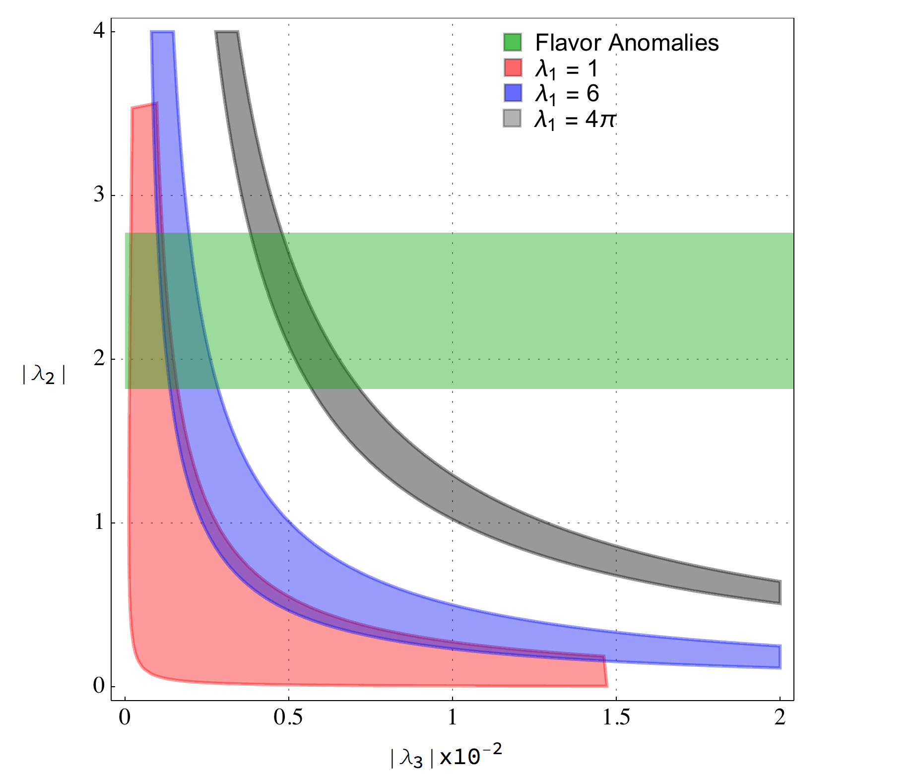
It can be seen from Fig. 2 that the resolution to flavor anomalies requires $\lambda_{2}\sim\mathcal{O}(1)$ whereas $\left(g-2\right)_{\mu}$ constrains $\lambda_{3}\sim\mathcal{O}(10^{-3})$ for $\lambda_{1}<6$ . Using this, and equations (32)-(36), one sees that the number of events at IceCube only depends on the coupling $\lambda_{1}$ . Since, $\Delta^{5/3}$ does not feature in the explanation for IceCube, these predictions are independent of $M_{1}$ and only depend on $M_{2}$ . In Fig. 3, we show the variation of the statistic $\delta$ with $M_{2}$ for various choice of coupling $\lambda_{1}$ . It can be seen that a Leptoquark of mass 800 - 1400 GeV can give 20-35% improvement to the fit. In Fig. 4, we show the contribution of Leptoquark for the benchmark point $M_{LQ}=$ 1 TeV, $\lambda_{1}\approx 6.$ which gives $\delta\simeq 35$ .

It is evident that for the aforementioned choices of Leptoquark parameters, one can satisfactorily explain the observed excess in the IceCube HESE Data. However, such an explanation requires large couplings and TeV scale Leptoquarks. Such a scenario should be testable at LHC and is the subject of study in the next section.

7 LHC constraints

Since Leptoquarks carry color charge, they can by singly or pair produced in pp collisions. Subsequent decays of these Leptoquarks in the detector will give rise to jets, leptons, and neutrinos. This gives very interesting final states of the form $jjll,~jjl\nu,~jl\nu,~jj\nu,~j\nu\nu$ , etc and has been the subject of various studies [64, 65, 66, 67, 68, 69, 70, 71, 72, 73, 74]. As these neutrinos are not seen by the detector, they appear as a Missing Transverse Energy (MET). For the LHC analysis, we have implemented the model using FeynRules (v2) [75] and simulate the above processes using MadGraph (v5)[76] which uses Pythia (v8) [77] for parton showering. We then use CheckMATE (v2) [78] to find the value of statistical parameter, r defined as

r=\frac{(S-1.96\Delta S)}{S_{exp}^{0.95}}

(39)

for several points in the parameter space. Here, $S$ and $\Delta S$ represents signal and its uncertainty. The numerator represents $95\%$ confidence limit on number of events obtained using CheckMATE and the denominator represents $95\%$ experimental limits on the number of events. The approximate functional form is obtained using linear interpolation. Parameter space with $r\geq 1$ is excluded and the results are summarized in Fig. 5.

Constraints from $jjll$ : When the Leptoquarks are pair produced in pp collisions, each Leptoquark can decay into a charged lepton and a quark. Recently, ATLAS collaboration performed a search for new physics signature of lepton-jet resonances based on $\sqrt{s}=13$ TeV data [79] wherein pair production of Leptoquarks was studied based on events like $eejj$ and $\mu\mu jj$ . The analysis gives an upper limit on branching ratio of first and second generation Leptoquark to $ej$ and $\mu j$ respectively. Although, our model has inter-generation couplings, we use these limits to constrain the free parameters in our model. We find that,

\mathcal{BR}\left(\Delta^{5/3}\to\mu j\right)\approx 1

(40)

as it couples to only second generation of leptons. This puts a lower limit on mass of Leptoquark as,

M_{1}\geq 1100~\text{TeV}.

We use the lower limit to generate other constraints and for flavor analysis. For $\Delta^{2/3}$ state,

\mathcal{BR}\left(\Delta^{2/3}\to\mu j\right)\propto\lambda_{4}^{2}\approx 0

(41)

which does not provide any constraints from this analysis.

Constraints from $jj\nu\nu$ : When the Leptoquark state $\Delta^{2/3}$ is pair produced, each can decay into a neutrino and a quark giving rise to a peculiar Dijet + MET signature. The parameters $M_{1}$ and $\lambda_{2}$ are fixed from flavor observables and this process only depends on $M_{2}$ and $\lambda_{1}$ . We use the 13 TeV ATLAS search [80] to find constraints on this parameter space.

Constraints from $j\nu\nu$ : If the Leptoquark $\Delta^{2/3}$ is singly produced, it can decay into a quark and a neutrino giving rise to Monojet signal at the LHC. Again, this process only depends on the parameters $M_{2}$ and $\lambda_{1}$ . We use the 8 TeV ATLAS search [81] to find constraints on this parameter space.

Other Constraints: We find that the Monojet constraints are strong enough to rule out the entire parameter space that explains IceCube PeV events and we do not provide results for other processes. However, in passing, we note that the constraints from $jl\nu$ final state are much stronger. This maybe relevant for future tests of Leptoquark models.

8 Conclusion

The discrepancy in anomalous magnetic moment of muon, the observed excess in PeV events at IceCube, and the lepton flavor universality violation in B decays are some of the biggest challenges facing the Standard Model. A simultaneous explanation for these problems is desirable. An ad-hoc solution such as Leptoquarks, if it can successfully address these issues, will shed more light on the unification scenarios that contain them. One such attempt was made in this paper using a scalar doublet Leptoquark. The peculiar feature of this model is that the flavor anomalies are explained at one-loop level. Because of the loop suppression, one does not require either very small couplings or very heavy Leptoquarks. We find that one can explain the B-anomalies $R_{K}$ and $R_{K^{*}}$ with $\mathcal{O}(1)$ coupling and TeV scale Leptoquark. In the past, similar parameters have been invoked to explain IceCube events and a unified explanation seemed possible. However, we find that in order to explain IceCube data, one needs Leptoquark coupling to first generation quarks and neutrinos. This coupling will give rise to Monojet and Dijet signals at LHC, both of which are severely constrained. Because of this, any attempt to explain IceCube events using such Leptoquarks would be in conflict with LHC data. This conclusion was also reached for a Scalar Triplet in [38], and for Scalar Singlet in [71]. Any unification scenario that has Leptoquark like states, IceCube explanation in such theories (e.g. R-Parity Violating MSSM [43]) should also be in conflict.

Acknowledgements

The authors would like to thank Prof. Namit Mahajan and Prof. Subhendra Mohanty for invaluable discussions and suggestions. The authors also thank the anonymous referee for pointing out the important LHC constraints on the model.

References

[1] Edward Farhi and Leonard Susskind. Technicolour. Physics Reports, 74(3):277–321, 1981.
[2] H. Georgi and S. L. Glashow. Unity of All Elementary Particle Forces. Physical Review Letters, 32:438–441, 1974.
[3] Howard Georgi. The State of the Art—Gauge Theories. AIP Conf. Proc., 23:575–582, 1975.
[4] Peter Cox, Alexander Kusenko, Olcyr Sumensari, and Tsutomu T. Yanagida. SU(5) Unification with TeV-scale Leptoquarks. JHEP, 03:035, 2017.
[5] Roel Aaij et al. Test of lepton universality using $B^{+}\rightarrow K^{+}\ell^{+}\ell^{-}$ decays. Phys. Rev. Lett., 113:151601, 2014.
[6] R. Aaij et al. Test of lepton universality with $B^{0}\rightarrow K^{*0}\ell^{+}\ell^{-}$ decays. 2017.
[7] Gudrun Hiller and Martin Schmaltz. $R_{K}$ and future $b\to s\ell\ell$ physics beyond the standard model opportunities. Phys. Rev., D90:054014, 2014.
[8] Guido D’Amico, Marco Nardecchia, Paolo Panci, Francesco Sannino, Alessandro Strumia, Riccardo Torre, and Alfredo Urbano. Flavour anomalies after the $R_{K^{*}}$ measurement. 2017.
[9] Damir Bečirević and Olcyr Sumensari. A leptoquark model to accommodate $R_{K}^{\mathrm{exp}}<R_{K}^{\mathrm{SM}}$ and $R_{K^{\ast}}^{\mathrm{exp}}<R_{K^{\ast}}^{\mathrm{SM}}$ . 2017.
[10] Gudrun Hiller and Ivan Nisandzic. $R_{K}$ and $R_{K^{\ast}}$ beyond the Standard Model. 2017.
[11] Yi Cai, John Gargalionis, Michael A. Schmidt, and Raymond R. Volkas. Reconsidering the One Leptoquark solution: flavor anomalies and neutrino mass. 2017.
[12] Andreas Crivellin, Dario Müller, and Toshihiko Ota. Simultaneous Explanation of $R(D^{(*)})$ and $b\to s\mu^{+}\mu^{-}$ : The Last Scalar Leptoquarks Standing. 2017.
[13] N. G. Deshpande and Xiao-Gang He. Consequences of R-parity violating interactions for anomalies in $\bar{B}\to D^{(*)}\tau\bar{\nu}$ and $b\to s\mu^{+}\mu^{-}$ . Eur. Phys. J., C77(2):134, 2017.
[14] Diganta Das, Chandan Hati, Girish Kumar, and Namit Mahajan. Scrutinizing $R$ -parity violating interactions in light of $R_{K^{(\ast)}}$ data. 2017.
[15] Sanjoy Biswas, Debtosh Chowdhury, Sangeun Han, and Seung J. Lee. Explaining the lepton non-universality at the LHCb and CMS within a unified framework. JHEP, 02:142, 2015.
[16] Wolfgang Altmannshofer, P. S. Bhupal Dev, and Amarjit Soni. $R_{D^{(*)}}$ anomaly: A possible hint for natural supersymmetry with $R$ -parity violation. 2017.
[17] Chandan Hati, Girish Kumar, and Namit Mahajan. $\bar{B}\rightarrow D^{(\ast)}\tau\bar{\nu}$ excesses in ALRSM constrained from $B$ , $D$ decays and $D^{0}-\bar{D}^{0}$ mixing. JHEP, 01:117, 2016.
[18] Ashutosh Kumar Alok, Bhubanjyoti Bhattacharya, Alakabha Datta, Dinesh Kumar, Jacky Kumar, and David London. New Physics in $b\to s\mu^{+}\mu^{-}$ after the Measurement of $R_{K^{*}}$ . 2017.
[19] Filippo Sala and David M. Straub. A New Light Particle in B Decays? 2017.
[20] Alakabha Datta, Jiajun Liao, and Danny Marfatia. A light $Z^{\prime}$ for the $R_{K}$ puzzle and nonstandard neutrino interactions. Phys. Lett., B768:265–269, 2017.
[21] Alakabha Datta, Jacky Kumar, Jiajun Liao, and Danny Marfatia. New light mediators for the $R_{K}$ and $R_{K^{*}}$ puzzles. 2017.
[22] Alejandro Celis, Javier Fuentes-Martin, Avelino Vicente, and Javier Virto. Gauge-invariant implications of the LHCb measurements on Lepton-Flavour Non-Universality. 2017.
[23] Marco Ciuchini, Antonio M. Coutinho, Marco Fedele, Enrico Franco, Ayan Paul, Luca Silvestrini, and Mauro Valli. On Flavourful Easter eggs for New Physics hunger and Lepton Flavour Universality violation. 2017.
[24] Li-Sheng Geng, Benjamín Grinstein, Sebastian Jäger, Jorge Martin Camalich, Xiu-Lei Ren, and Rui-Xiang Shi. Towards the discovery of new physics with lepton-universality ratios of $b\to s\ell\ell$ decays. 2017.
[25] T. Hurth, F. Mahmoudi, and S. Neshatpour. Global fits to $b\to s\ell\ell$ data and signs for lepton non-universality. JHEP, 12:053, 2014.
[26] Cheng-Wei Chiang, Xiao-Gang He, Jusak Tandean, and Xing-Bo Yuan. $R_{K^{(*)}}$ and related $b\to s\ell\bar{\ell}$ anomalies in minimal flavor violation framework with $Z^{\prime}$ boson. 2017.
[27] Andreas Crivellin, Giancarlo D’Ambrosio, and Julian Heeck. Addressing the LHC flavor anomalies with horizontal gauge symmetries. Phys. Rev., D91(7):075006, 2015.
[28] Diptimoy Ghosh. Explaining the $R_{K}$ and $R_{K^{*}}$ anomalies. 2017.
[29] Cesar Bonilla, Tanmoy Modak, Rahul Srivastava, and Jose W. F. Valle. $U(1)_{B_{3}-3L_{\mu}}$ gauge symmetry as the simplest description of $b\to s$ anomalies. 2017.
[30] James M. Cline and Jorge Martin Camalich. $B$ decay anomalies from nonabelian local horizontal symmetry. 2017.
[31] G. Couture and H. Konig. Bounds on second generation scalar leptoquarks from the anomalous magnetic moment of the muon. Phys. Rev., D53:555–557, 1996.
[32] Estefania Coluccio Leskow, Giancarlo D’Ambrosio, Andreas Crivellin, and Dario Müller. $(g-2)\mu$ , lepton flavor violation, and $Z$ decays with leptoquarks: Correlations and future prospects. Phys. Rev., D95(5):055018, 2017.
[33] Seungwon Baek and Kenji Nishiwaki. Leptoquark explanation of $h\to\mu\tau$ and muon $(g-2)$ . Phys. Rev., D93(1):015002, 2016.
[34] Diganta Das, Chandan Hati, Girish Kumar, and Namit Mahajan. Towards a unified explanation of $R_{D^{(\ast)}}$ , $R_{K}$ and $(g-2)_{\mu}$ anomalies in a left-right model with leptoquarks. Phys. Rev., D94:055034, 2016.
[35] King-man Cheung. Muon anomalous magnetic moment and leptoquark solutions. Phys. Rev., D64:033001, 2001.
[36] Chuan-Hung Chen, Takaaki Nomura, and Hiroshi Okada. Excesses of muon $g-2$ , $R_{D^{(\ast)}}$ , and $R_{K}$ in a leptoquark model. 2017.
[37] Vernon Barger and Wai-Yee Keung. Superheavy Particle Origin of IceCube PeV Neutrino Events. Phys. Lett., B727:190–193, 2013.
[38] Nicolas Mileo, Alejandro de la Puente, and Alejandro Szynkman. Implications of a Electroweak Triplet Scalar Leptoquark on the Ultra-High Energy Neutrino Events at IceCube. JHEP, 11:124, 2016.
[39] Ujjal Kumar Dey and Subhendra Mohanty. Constraints on Leptoquark Models from IceCube Data. JHEP, 04:187, 2016.
[40] Bhaskar Dutta, Yu Gao, Tianjun Li, Carsten Rott, and Louis E. Strigari. Leptoquark implication from the CMS and IceCube experiments. Phys. Rev., D91:125015, 2015.
[41] Luis A. Anchordoqui, Carlos A. Garcia Canal, Haim Goldberg, Daniel Gomez Dumm, and Francis Halzen. Probing leptoquark production at IceCube. Phys. Rev., D74:125021, 2006.
[42] Ujjal Kumar Dey, Subhendra Mohanty, and Gaurav Tomar. Leptoquarks: 750 GeV Diphoton Resonance and IceCube Events. 2016.
[43] P. S. Bhupal Dev, Dilip Kumar Ghosh, and Werner Rodejohann. R-parity Violating Supersymmetry at IceCube. Phys. Lett., B762:116–123, 2016.
[44] I. Doršner, S. Fajfer, A. Greljo, J. F. Kamenik, and N. Košnik. Physics of leptoquarks in precision experiments and at particle colliders. Phys. Rept., 641:1–68, 2016.
[45] Debrupa Chakraverty, Debajyoti Choudhury, and Anindya Datta. A Nonsupersymmetric resolution of the anomalous muon magnetic moment. Phys. Lett., B506:103–108, 2001.
[46] Geneviève Bélanger, Cédric Delaunay, and Susanne Westhoff. A Dark Matter Relic From Muon Anomalies. Phys. Rev., D92:055021, 2015.
[47] C. Patrignani and Particle Data Group. Review of particle physics. Chinese Physics C, 40(10):100001, 2016.
[48] Gudrun Hiller and Frank Kruger. More model-independent analysis of $b\to s$ processes. Phys. Rev., D69:074020, 2004.
[49] Bernat Capdevila, Andreas Crivellin, Sébastien Descotes-Genon, Joaquim Matias, and Javier Virto. Patterns of New Physics in $b\to s\ell^{+}\ell^{-}$ transitions in the light of recent data. 2017.
[50] Debjyoti Bardhan, Pritibhajan Byakti, and Diptimoy Ghosh. Role of Tensor operators in $R_{K}$ and $R_{K^{*}}$ . 2017.
[51] Wolfgang Altmannshofer, Patricia Ball, Aoife Bharucha, Andrzej J. Buras, David M. Straub, and Michael Wick. Symmetries and Asymmetries of $B\to K^{*}\mu^{+}\mu^{-}$ Decays in the Standard Model and Beyond. JHEP, 01:019, 2009.
[52] Hiren H. Patel. Package-X 2.0: A Mathematica package for the analytic calculation of one-loop integrals. Comput. Phys. Commun., 218:66–70, 2017.
[53] Li-Sheng Geng, Benjamín Grinstein, Sebastian Jäger, Jorge Martin Camalich, Xiu-Lei Ren, and Rui-Xiang Shi. Towards the discovery of new physics with lepton-universality ratios of $b\to s\ell\ell$ decays. 2017.
[54] Roel Aaij et al. Measurement of the $B^{0}_{s}\to\mu^{+}\mu^{-}$ branching fraction and effective lifetime and search for $B^{0}\to\mu^{+}\mu^{-}$ decays. Phys. Rev. Lett., 118(19):191801, 2017.
[55] Damir Bečirević, Olcyr Sumensari, and Renata Zukanovich Funchal. Lepton flavor violation in exclusive $b\rightarrow s$ decays. Eur. Phys. J., C76(3):134, 2016.
[56] Christoph Bobeth, Martin Gorbahn, Thomas Hermann, Mikolaj Misiak, Emmanuel Stamou, and Matthias Steinhauser. $B_{s,d}\to l^{+}l^{-}$ in the Standard Model with Reduced Theoretical Uncertainty. Phys. Rev. Lett., 112:101801, 2014.
[57] Carsten Rott, Kazunori Kohri, and Seong Chan Park. Superheavy dark matter and IceCube neutrino signals: Bounds on decaying dark matter. Phys. Rev., D92(2):023529, 2015.
[58] Nagisa Hiroshima, Ryuichiro Kitano, Kazunori Kohri, and Kohta Murase. High-energy Neutrinos from Multi-body Decaying Dark Matter. 2017.
[59] Atri Bhattacharya, Arman Esmaili, Sergio Palomares-Ruiz, and Ina Sarcevic. Probing decaying heavy dark matter with the 4-year IceCube HESE data. 2017.
[60] Sergio Palomares-Ruiz, Aaron C. Vincent, and Olga Mena. Spectral analysis of the high-energy IceCube neutrinos. Phys. Rev., D91(10):103008, 2015.
[61] Raj Gandhi, Chris Quigg, Mary Hall Reno, and Ina Sarcevic. Ultrahigh-energy neutrino interactions. Astropart. Phys., 5:81–110, 1996.
[62] M. G. Aartsen et al. The IceCube Neutrino Observatory - Contributions to ICRC 2015 Part II: Atmospheric and Astrophysical Diffuse Neutrino Searches of All Flavors. In Proceedings, 34th International Cosmic Ray Conference (ICRC 2015): The Hague, The Netherlands, July 30-August 6, 2015, 2015.
[63] A. D. Martin, W. J. Stirling, R. S. Thorne, and G. Watt. Parton distributions for the LHC. Eur. Phys. J., C63:189–285, 2009.
[64] Oscar J. P. Eboli, R. Zukanovich Funchal, and T. L. Lungov. Signal and backgrounds for leptoquarks at the CERN LHC. Phys. Rev., D57:1715–1729, 1998.
[65] M. Kramer, T. Plehn, M. Spira, and P. M. Zerwas. Pair production of scalar leptoquarks at the CERN LHC. Phys. Rev., D71:057503, 2005.
[66] Alexander Belyaev, Claude Leroy, Rashid Mehdiyev, and Alexander Pukhov. Leptoquark single and pair production at LHC with CalcHEP/CompHEP in the complete model. JHEP, 09:005, 2005.
[67] Ilja Dorsner, Svjetlana Fajfer, and Admir Greljo. Cornering Scalar Leptoquarks at LHC. JHEP, 10:154, 2014.
[68] Tanumoy Mandal, Subhadip Mitra, and Satyajit Seth. Single Productions of Colored Particles at the LHC: An Example with Scalar Leptoquarks. JHEP, 07:028, 2015.
[69] Tanumoy Mandal, Subhadip Mitra, and Satyajit Seth. Pair Production of Scalar Leptoquarks at the LHC to NLO Parton Shower Accuracy. Phys. Rev., D93(3):035018, 2016.
[70] Ilja Dorsner. Scalar leptoquarks at LHC. PoS, CORFU2015:051, 2016.
[71] Ujjal Kumar Dey, Deepak Kar, Manimala Mitra, Michael Spannowsky, and Aaron C. Vincent. Searching for Leptoquarks at IceCube and the LHC. 2017.
[72] Priyotosh Bandyopadhyay and Rusa Mandal. Revisiting scalar leptoquark at the LHC. 2018.
[73] Ilja Dorsner and Admir Greljo. Leptoquark toolbox for precision collider studies. 2018.
[74] Gudrun Hiller, Dennis Loose, and Ivan Nisandzic. Flavorful leptoquarks at hadron colliders. 2018.
[75] Adam Alloul, Neil D. Christensen, Celine Degrande, Claude Duhr, and Benjamin Fuks. FeynRules 2.0 - A complete toolbox for tree-level phenomenology. Comput. Phys. Commun., 185:2250–2300, 2014.
[76] J. Alwall, R. Frederix, S. Frixione, V. Hirschi, F. Maltoni, O. Mattelaer, H. S. Shao, T. Stelzer, P. Torrielli, and M. Zaro. The automated computation of tree-level and next-to-leading order differential cross sections, and their matching to parton shower simulations. JHEP, 07:079, 2014.
[77] Torbjorn Sjostrand, Stefan Ask, Jesper R. Christiansen, Richard Corke, Nishita Desai, Philip Ilten, Stephen Mrenna, Stefan Prestel, Christine O. Rasmussen, and Peter Z. Skands. An Introduction to PYTHIA 8.2. Comput. Phys. Commun., 191:159–177, 2015.
[78] Manuel Drees, Herbi Dreiner, Daniel Schmeier, Jamie Tattersall, and Jong Soo Kim. CheckMATE: Confronting your Favourite New Physics Model with LHC Data. Comput. Phys. Commun., 187:227–265, 2015.
[79] Morad Aaboud et al. Search for scalar leptoquarks in pp collisions at $\sqrt{s}$ = 13 TeV with the ATLAS experiment. New J. Phys., 18(9):093016, 2016.
[80] Morad Aaboud et al. Search for squarks and gluinos in final states with jets and missing transverse momentum at $\sqrt{s}=$ 13 TeV with the ATLAS detector. Eur. Phys. J., C76(7):392, 2016.
[81] Georges Aad et al. Search for new phenomena in final states with an energetic jet and large missing transverse momentum in pp collisions at $\sqrt{s}=$ 8 TeV with the ATLAS detector. Eur. Phys. J., C75(7):299, 2015. [Erratum: Eur. Phys. J.C75,no.9,408(2015)].