Supplementary Materials:
Dueling Bandits with Weak Regret
Abstract
We consider online content recommendation with implicit feedback through pairwise comparisons, formalized as the so-called dueling bandit problem. We study the dueling bandit problem in the Condorcet winner setting, and consider two notions of regret: the more well-studied strong regret, which is 0 only when both arms pulled are the Condorcet winner; and the less well-studied weak regret, which is 0 if either arm pulled is the Condorcet winner. We propose a new algorithm for this problem, Winner Stays (WS), with variations for each kind of regret: WS for weak regret (WS-W) has expected cumulative weak regret that is , and if arms have a total order; WS for strong regret (WS-S) has expected cumulative strong regret of , and if arms have a total order. WS-W is the first dueling bandit algorithm with weak regret that is constant in time. WS is simple to compute, even for problems with many arms, and we demonstrate through numerical experiments on simulated and real data that WS has significantly smaller regret than existing algorithms in both the weak- and strong-regret settings.
Keywords:
boring formatting information, machine learning, ICML1 Introduction
We consider bandit learning in personalized content recommendation with implicit pairwise comparisons. We offer pairs of items to a user and record implicit feedback on which offered item is preferred, seeking to learn the user’s preferences over items quickly, while also ensuring that the fraction of time we fail to offer a high-quality item is small. Implicit pairwise comparisons avoid the inaccuracy of user ratings (Joachims et al., 2007) and the difficulty of engaging users in providing explicit feedback.
We study a model for this setting called the dueling bandit problem (Yue & Joachims, 2009). The items we may offer to the user are called “arms”, and we learn about these arms through a sequence of “duels”. In each duel, we “pull” two arms and receive noisy feedback from the user telling us which arm is preferred. When an arm is preferred within a duel, we say that the arm has “won the duel".
We study this problem in the Condorcet winner setting, in which we assume the existence of an arm (the Condorcet winner) that wins with probability at least when paired with any of the other arms. In these settings, we consider two notions of regret: “weak regret“, in which we avoid regret by selecting the Condorcet winner as either arm in the duel; and “strong-regret”, in which we can only avoid regret by setting both arms in the duel to the Condorcet winner.
Weak regret was proposed by Yue et al. (2012) and arises in content recommendation when arms correspond to items, and the user incurs no regret whenever his most preferred item is made available. Examples include in-app restaurant recommendations provided by food delivery services like Grubhub and UberEATS, in which implicit feedback may be inferred from selections, and the user only incurs regret if her most preferred restaurant is not recommended. Examples also include recommendation of online broadcasters on platforms such as Twitch, in which implicit feedback may again be inferred from selections, and the user is fully satisfied as long as her favored broadcaster is listed. Despite its applicability, Yue et al. (2012) is the only paper of which we are aware that studies weak regret, and it does not provide algorithms specifically designed for this setting.
Strong regret has been more widely studied, as discussed below, and has application to choosing ranking algorithms for search (Hofmann et al., 2013). To perform a duel, query results from two rankers are interleaved (Radlinski et al., 2008), and the ranking algorithm that provided the first result chosen by the user is declared the winner of the duel. Strong regret is appropriate in this setting because the user’s experience is enhanced by pulling the best arm twice, so that all of that ranker’s results are shown.
Our contribution is a new algorithm, Winner Stays (WS), with variants designed for the weak (WS-W) and strong regret (WS-S) settings. We prove that WS-W has expected cumulative weak regret that is constant in time, with dependence on the number of arms given by . If the arms have a total order, we show a tighter bound of . We then prove that WS-S has expected cumulative strong regret that is , and prove that a tighter bound of holds if arms have a total order. These regret bounds are optimal in , and for weak regret are strictly better than those for any previously proposed algorithm, although at the same time both strong and weak regret bounds are sensitive to the minimum gap in winning probability between arms. We demonstrate through numerical experiments on simulated and real data that WS-W and WS-S significantly outperform existing algorithms on strong and weak regret.
The paper is structured as follows. Section 2 reviews related work. Section 3 formulates our problem. Section 4 introduces the Winner Stays (WS) algorithm: Section 4.1 defines WS-W for the weak regret setting; Section 4.2 proves that WS-W has cumulative expected regret that is constant in time; Section 4.3 defines WS-S for the strong regret setting and bounds its regret. Section 4.4 disusses a simple extension of our theoretical results to the utility-based bandit setting, which is used in our numerical experiments. Section 5 compares WS with three benchmark algorithms using both simulated and real datasets, finding that WS outperforms these benchmarks on the problems considered.
2 Related Work
Most work on dueling bandits focuses on strong regret. Yue et al. (2012) shows that the worst-case expected cumulative strong regret up to time T for any algorithm is . Algorithms have been proposed that reach this lower bound under the Condorcet winner assumption in the finite-horizon setting: Interleaved Filter (IF) (Yue et al., 2012) and Beat the Mean (BTM) (Yue & Joachims, 2011). Relative Upper Confidence Bound (RUCB) (Zoghi et al., 2014) also reaches this lower bound in the horizonless setting. Relative Minimum Empirical Divergence (RMED) (Komiyama et al., 2015) is the first algorithm to have a regret bound that matches this lower bound. Zoghi et al. (2015) proposed two algorithms, Copeland Confidence Bound (CCB) and Scalable Copeland Bandits (SCB), which achieve an optimal regret bound without assuming existence of a Condorcet winner.
While weak regret was proposed in Yue et al. (2012), it has not been widely studied to our knowledge, and despite its applicability we are unaware of papers that provide algorithms designed for it specifically. While one can apply algorithms designed for the strong regret setting to weak regret, and use the fact that strong dominates weak regret to obtain weak regret bounds of , these are looser than the constant-in- bounds that we show.
Active learning using pairwise comparisons is also closely related to our work. Jamieson & Nowak (2011) considers an active learning problem that is similar to our problem in that the primary goal is to sort arms based on the user’s preferences, using adaptive pairwise comparisons. It proposes a novel algorithm, the Query Selection Algorithm (QSA), that uses an expected number of operations of to sort arms, where is the dimension of the space in which the arms are embedded, rather than . Busa-Fekete et al. (2013) and Busa-Fekete et al. (2014) consider top-k element selection using adaptive pairwise comparisons. They propose a generalized racing algorithm focusing on minimizing sample complexity. (Pallone et al., 2017) studies adaptive preference learning across arms using pairwise preferences. They show that a greedy algorithm is Bayes-optimal for an entropy objective. While similar in that they use pairwise comparisons, these algorithms are different in focus from the current work because they do not consider cumulative regret.
3 Problem Formulation
We consider items (arms). At each time , the system chooses two items and shows them to the user, i.e., the system performs a duel between two arms. The user then provides binary feedback indicating her preferred item, determining which arm wins the duel. This binary feedback is random, and is conditionally independent of all past interactions given the pair of arms shown. We let denote the probability that the user gives feedback indicating a preference for arm , when shown arms and . If the user prefers arm over arm , we assume . We also assume symmetry: .
We assume arm is a Condorcet winner, i.e., that for . In some results, we also consider the setting in which arms have a total order, by which we mean that the arms are ordered so that for all . The total order assumption implies transitivity.
We let be a lower bound on the probability that the user will choose her favourite arm.
We consider both weak and strong regret in its binary form. The single-period weak regret incurred at this time is if we do not pull the best arm and otherwise. The single-period strong regret is if we do not pull the best arm twice and otherwise. We also consider utility-based extensions of weak and strong regret in Section 4.4.
We use the same notation to denote strong and weak regret, and rely on context to distinguish the two cases. In both cases, we define the cumulative regret up to time to be . We measure the quality of an algorithm by its expected cumulative regret.
4 Winner Stays
We now propose an algorithm, called Winner Stays (WS), with two variants: WS-W designed for weak regret; and WS-S for strong regret. Section 4.1 introduces WS-W and illustrates its dynamics. Section 4.2 proves the expected cumulative weak regret of WS-W is under the Condorcet winner setting, and under the total order setting. Section 4.3 introduces WS-S and proves that its expected cumulative strong regret is under the Condorcet winner setting, and under the total order setting, both of which have optimal dependence on . Section 4.4 extends our theoretical results to utility-based bandits.
4.1 Winner Stays with Weak Regret (WS-W)
We now present WS-W, first defining some notation. Let be the number of times that arm has defeated arm in a duel, up to and including time . Then, define . is the difference between the number of duels won and lost by arm , up to time . With this notation, we define WS-W in Algorithm 1.
Input: arms
for do
- •
If and , set .
- •
Else if and , set .
- •
Else choose uniformly at random from .
- •
If and , set .
- •
Else if and , set .
- •
Else choose uniformly at random from .
Step 4: Observe noisy binary feedback and update and ;
WS-W’s pulls can be organized into iterations, each of which consists of a sequence of pulls of the same pair of arms, and rounds, each of which consists of a sequence of iterations in which arms that lose an iteration are not visited again until the next round. We first describe iterations and rounds informally with an example and in Figure 1 before presenting our formal analysis.
Example: At time , for all , and WS-W pulls two randomly chosen arms. Suppose it pulls arms , and arm wins. Then is 1 for arm 1, for arm 2, and for the other arms. This first pull is an iteration of length 1, arm is the winner, and arm is the loser. This iteration is in the first round. We call the start of the first round, and the start of the first iteration in the first round.
At time , is largest for arm so WS-W chooses . Since is for arm 2 and 0 for the other arms, WS-W chooses at random from arms 3 through (suppose ). Suppose it chooses arm . This pair of arms (1 and 3) is different from the pair pulled in the previous iteration (1 and 2), so is the start of the second iteration (in the first round).
WS-W continues pulling arms 1 and 3 until is for one of these arms and for the other. WS-W continues to pull only arms 1 and 3 until one has even though this may involve times when is 0 for both arms 1 and 3, causing them to be tied with arms 4 and above, because we break ties to prioritize pulling previously pulled arms. The sequence of times when we pull arms 1 and 3 is the second iteration. The arm that ends the iteration with is the winner of that iteration.

WS-W continues this process, performing iterations on different pairs of arms, pitting the winner of each iteration against a previously unplayed arm in the next iteration. This sequence of iterations is the first round. The winner of the final iteration in the first round, call it arm , has and all other arms have .
The second round begins on the next pull after the end of the first round, at time . WS-W again performs iterations, playing in the first iteration. Each iteration has a winner that passes to the next iteration.
WS-W repeats this process for an infinite number of rounds. Each round is a sequence of iterations, and an arm that loses an iteration is not revisited until the next round. Figure 1 illustrates these dynamics, and we formalize the definition of round and iteration in the next section.
4.2 Analysis of WS-W
In this section, we analyze the weak regret of WS-W. After presenting definitions and preliminary results, we prove WS-W has expected cumulative weak regret bounded by when arms have a total order. Then, in the more general Condorcet winner setting, we prove WS-W has expected cumulative weak regret bounded by . We leave the proofs of all lemmas to the supplement.
We define , the beginning of round , and , the winner of round , as the unique time and arm such and for all .
We define , the beginning of iteration in round , as the first time we pull the unique pair of arms in the round. We let be the number of successive pulls of this pair of arms.
We additionally define terminology to describe arms pulled in an iteration. In a duel between arms and with , arm is called the better arm and arm is called the worse arm. We say that an arm is the incumbent in iteration iteration and round if . A unique such arm exists except when . When , the incumbent is the better of the two arms being played. We call the arm being played that is not the incumbent the challenger.
Using these definitions, we present our first pair of results toward bounding the expected cumulative weak regret of WS-W. They bound the number of pulls in an iteration.
Lemma 1.
The conditional expected length of iteration in round , given the arms being pulled, is bounded above by if the incumbent is worse than the challenger, and by if the incumbent is better than the challenger.
Lemma 1 shows that iterations with a worse incumbent use more pulls. We then bound the number of iterations with a worse incumbent.
Lemma 2.
Under the total order assumption, the conditional expected number of future iterations with an incumbent worse than the challenger, given history up to time , is bounded above by for any .
Lemma 2 implies that the incumbent is worse than the challenger in finitely many iterations with probability . We now bound the tail distribution of the last such round.
Lemma 3.
Let denote the smallest such that no round contains an iteration in which the incumbent is worse than the challenger. Then .
To present our final set of preliminary lemmas, we define several indicator functions. Let be when the incumbent in iteration of round is better than the challenger. Let be if arm 1 (the best arm) is the incumbent at the beginning of iteration 1 of round . Denote and . Let be if and arm loses in any iteration through of round .
We may only incur weak regret during round iteration if , or if for some . We will separately bound the regret incurred in these two different scenarios. Moreover, our bound on the number of pulls, and thus the regret incurred, in this iteration will depend on whether or . This leads us to state four inequalities in the following pair of lemmas, which we will in turn use to show Theorem 1. The first lemma applies in both the total order and Condorcet settings, while the second applies only in the total order setting. When proving Theorem 2 we replace Lemma 5 by an alternate pair of inequalities.
Lemma 4.
Lemma 5.
Under the total order assumption:
- •
is bounded above by .
- •
is bounded above by .
We now state our main result for the total order setting, which shows that the expected cumulative weak regret is .
Theorem 1.
The expected cumulative weak regret of WS-W is bounded by under the total order assumption.
Proof.
Iterations can be divided into two types: those in which the incumbent is better than the challenger, and those where the incumbent is worse.
We first bound expected total weak regret incurred in the first type of iteration, and then below bound that incurred in the second type. In this first bound, observe that we incur weak regret during round if , or if but arm loses to some other arm during this round. Under the second scenario, we do not incur any regret until arm loses to another arm.
Thus, the expected weak regret incurred during iterations with a better incumbent is bounded by
The first part of this summation can be bounded by the first inequality in Lemma 4 to obtain
The second part of this summation can be bounded by the second inequality in Lemma 4 to obtain
Thus, the cumulative expected weak regret incurred during iterations with a better incumbent is bounded by .
Now we bound the expected weak regret incurred during iterations where the incumbent is worse than the challenger. This is bounded by
The first term in the summation can be bounded by the first inequality of Lemma 5 to obtain
The second term in the summation can be bounded by the first inequality of Lemma 5 to obtain
Thus, the cumulative expected weak regret incurred during iterations with a worse incumbent is bounded by .
Summing these two bounds, the cumulative expected weak regret is bounded by . ∎
We prove the following result for the Condorcet winner setting in a similar manner in the supplement.
Theorem 2.
The expected cumulative weak regret of WS-W is bounded by under the Condorcet winner setting.
4.3 Winner Stays with Strong Regret (WS-S)

In this section, we define a version of WS for strong regret, WS-S, which uses WS-W as a subroutine. WS-S is defined in Algorithm 2
Input: , arms
for do
Exploitation phase: Let be the index of the best arm at the end of the round. For the next time periods, pull arms and and ignore the feedback.
Each round of WS-S consists of an exploration phase and an exploitation phase. The length of the exploitation phase increases exponentially with the number of phases. Changing the parameter balances the lengths of these phases, and thus balances between exploration and exploitation. Our theoretical results below guide choosing .
We now bound the cumulative strong regret of this algorithm under both the total order and Condorcet winner settings:
Theorem 3.
If there is a total order among arms, then for , the expected cumulative strong regret for WS-S is bounded by .
Proof.
Suppose at time T, we are in round . Then . Solving for , we obtain .
We bound the expected strong regret up to time . The expected regret can be divided in two parts: the regret occuring during the exploration phase; and the regret occuring during the exploitation phase.
First we focus on regret incurred during exploration. We never pull the same arm twice during this phase, and so regret is incurred in each time period. To bound regret incurred during exploration, we bound the length of time spent in this phase.
The length of time spent in exploration up to the end of round with a better incumbent is bounded by . The length of time spent with a worse incumbent, based on the proof of Theorem 1, is bounded by .
Now we focus on regret incurred during exploitation. The probability we have identified the wrong arm at the end of the round is less than . Thus, the expected regret incurred during this phase up until the end of the round is bounded by .
Overall, this implies that the strong expected regret up to time (recall that is in round ) is bounded by
Thus, the expected strong regret up to time is . ∎
Theorem 4.
Under the Condorcet winner setting and for , the expected cumulative strong regret for WS-S is bounded by .
Proof.
These results provide guidance on the choice of . If is too close to 1, then we spend most of the time in the exploration phase, which is guaranteed to generate strong regret. The last inequality in the proof of Theorem 3 suggests that asymptotic regret will be smallest if we choose as large as possible without going beyond the threshold. Indeed, if is too large, then WS-S may incur large regret in early exploitation stages when we have finished only a few rounds of exploration. In our numerical experiments we set , which satisfies the constraint assumed by our theory if . With a properly chosen , the numerical experiments in section 5.2 suggest WS-S performs better than previously devised algorithms. At the same time, the best choice of is dependent on . Modifying WS-S to eliminate parameters that must be chosen with knowledge of is left for future work.
Our regret bound grows as , which is the minimal gap between two arms, shrinks, and tends to decrease as the number of arms increases. Other dueling bandit algorithm for strong regret, such as RUCB and RMED, have regret bounds with better dependence on the gaps between arms. Modifying WS-S to provide improved dependence on these gaps is also left for future work.
4.4 Extension to Utility-Based Regret
We now briefly discuss utility-based extensions of weak and strong regret for the total order setting, following utility-based bandits studied in Ailon et al. (2014). Our regret bounds also apply here, with a small modification.
Suppose that the user has a utility associated with each arm . Without loss of generality, we assume , and as in the total order setting, we require that when . Typically the would come from the utilities of arms and via a generative model. We give an example in our numerical experiments.
Then, the single-period utility-based weak regret is , which is the difference in utility between the best arm overall and the best arm that the user can choose from those offered. The single-period utility-based strong regret is . To get zero regret under strong regret, the best arm must be pulled twice.
Our results from Section 4 carry through to this more general regret setting. Let be the maximum single-period regret. Then, the expected cumulative utility-based weak regret for WS-W is , and the expected cumulative utility-based strong regret for WS-S is .
5 Numerical Experiments
In this section, we evaluate WS under both the weak and strong regret settings, considering both their original (binary) and utility-based versions. In the weak regret setting, we compare WS-W with RUCB and QSA. In the strong regret setting, we compare WS-S with 7 benchmarks including RUCB and Relative Minimum Empirical Divergence (RMED) by Komiyama et al. (2015). We also include an experiment violating the total order assumption in Section 11 in the supplement. WS outperforms all benchmarks tested in these numerical experiments.


5.1 Weak Regret
We now compare WS-W with QSA and RUCB using simulated data and the Yelp academic dataset (Yelp, 2012).
5.1.1 Simulated Data
In this example, we compare WS-W with RUCB and QSA on a problem with arms and binary weak regret. Each arm is a 20-dimensional vector uniformly generated from the unit circle. We assume for all .
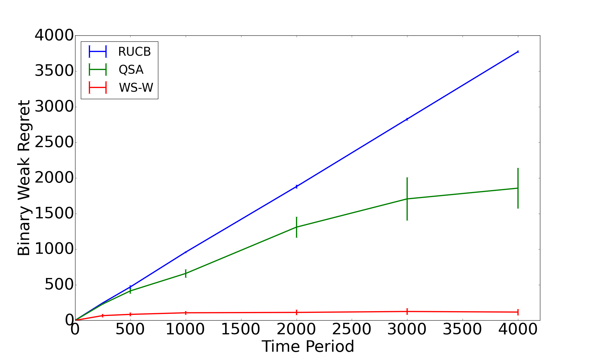
The results are summarized in Figure 2(a). RUCB has approximately linear regret over the time horizon pictured. This is common in the dueling bandits literature, where many algorithms require comparisons before they achieve cumulative regret for arms. WS-W finds the optimal arm after comparisons and has a regret that is consistent with our theoretically established constant expected cumulative weak regret.
5.1.2 Yelp Academic Dataset
In this example, we compare WS-W with RUCB and QSA using the Yelp academic dataset (Yelp, 2012) and utility-based weak regret.
We choose restaurants from Las Vegas as our arms. Associated with each arm (restaurant) is a -dimensional feature vector , calculated using doc2vec (Rehurek & Sojka, 2010) from its reviews. We select 49 users who have reviewed at least of these restaurants. For each user, we model their utility for restaurant as , where is a -dimensional vector of preferences. We infer for each user using linear regression.
To model , we then use the probit model. We let be the estimated variance of the residuals from the linear regression above. When presented with two restaurants, we model the user as taking independent random draws from a normal distribution with means and respectively and variances , and choosing the restaurant with the larger draw. This gives , where is the cdf for the normal distribution with mean 0 and variance .
We simulate performance for each user separately, and then average the results. These results are summarized in Figure 2(b). WS-W outperforms RUCB and QSA, finding the optimal restaurant after iterations.
5.2 Strong Regret
In this section, we compare WS-S using binary and utility-based strong regret with 7 benchmarks from the literature. We use the sushi and MSLR datasets, which were previously used by Komiyama et al. (2016) and Zoghi et al. (2015) respectively to evaluate dueling bandit algorithms.
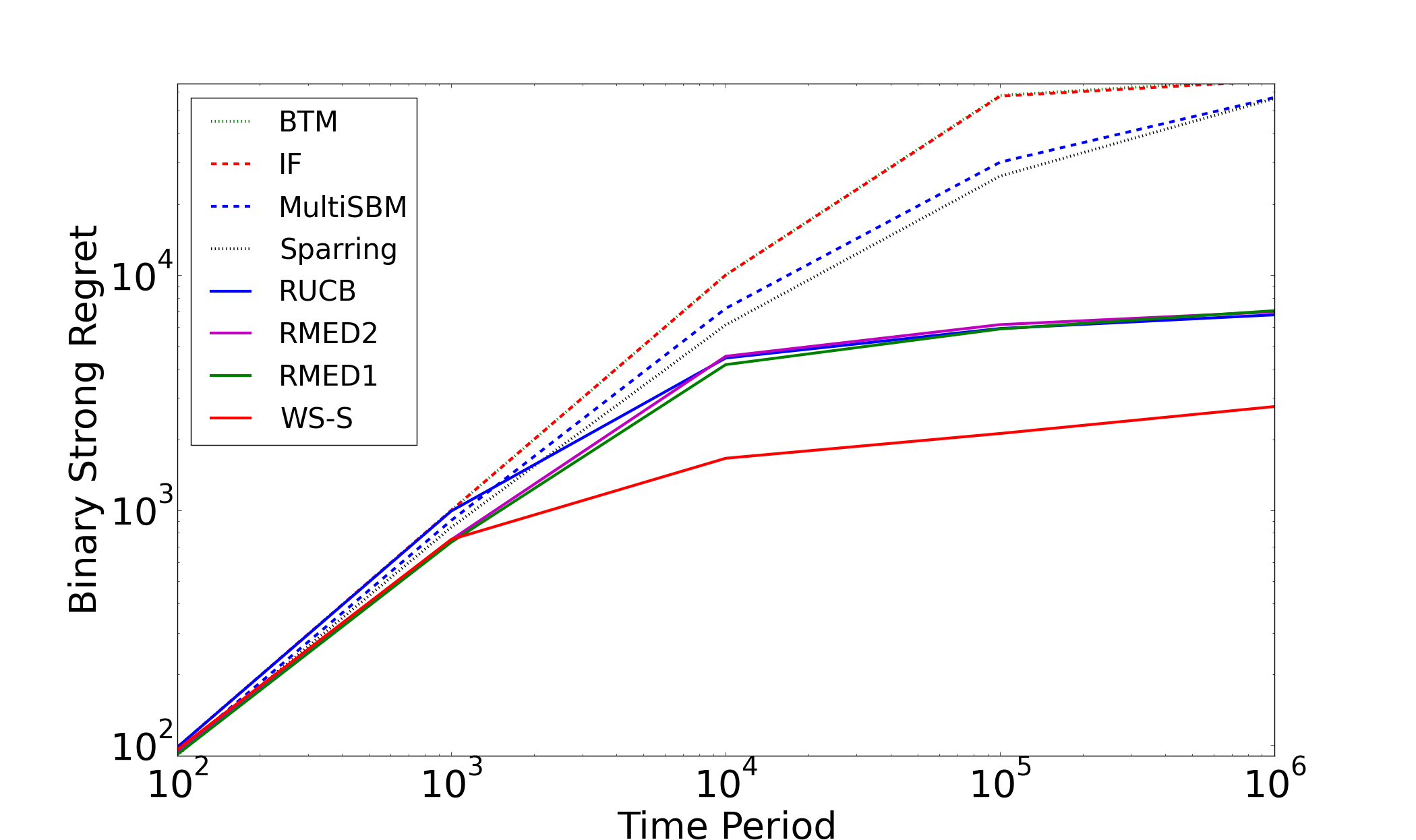
The sushi dataset (Komiyama et al., 2016) contains 16 arms corresponding to types of sushi, with pairwise preferences inferred from data on sushi preferences from 5000 users in Kamishima (2003). The MSLR dataset has 5 arms, corresponding to ranking algorithms, with pairwise preferences provided in Zoghi et al. (2015). We give preference matrices for both datasets in the supplement. For utility-based regret, we define .
WS-S has a user-defined parameter . In our experiments we set . The corresponding minimum for which our theoretical bounds hold is . We recommend for problems of arms or fewer, and closer to 1 for those problems with more arms that are likely to have closer to . We also conduct a sensitivity analysis of in the supplement.
Figure 3 shows the results of our comparisons. WS-S outperforms all 7 benchmarks considered on both datasets using both variants of strong regret.
6 Conclusion
In this paper, we consider dueling bandits for online content recommendation using both weak and strong regret.
We propose a new algorithm, WS, with variants designed for the weak regret (WS-W) and strong regret (WS-S) settings. We prove WS has constant weak regret and optimal strong regret in . In numerical experiments, WS outperforms all benchmarks considered on both simulated and real datasets.
Acknowledgements
The authors were partially supported by NSF CAREER CMMI-1254298, NSF CMMI-1536895, NSF IIS-1247696, NSF DMR-1120296, AFOSR FA9550-12-1-0200, AFOSR FA9550-15-1-0038, and AFOSR FA9550-16-1-0046.
References
- Ailon et al. (2014) Ailon, Nir, Karnin, Zohar Shay, and Joachims, Thorsten. Reducing dueling bandits to cardinal bandits. In ICML, volume 32, pp. 856–864, 2014.
- Barndorff-Nielsen & Shiryaev (2015) Barndorff-Nielsen, Ole E and Shiryaev, Albert. Change of time and change of measure, volume 21. World Scientific Publishing Co Inc, 2015.
- Busa-Fekete et al. (2013) Busa-Fekete, Róbert, Szörényi, Balázs, Cheng, Weiwei, Weng, Paul, and Hüllermeier, Eyke. Top-k selection based on adaptive sampling of noisy preferences. In ICML (3), pp. 1094–1102, 2013.
- Busa-Fekete et al. (2014) Busa-Fekete, Róbert, Hüllermeier, Eyke, and Szörényi, Balázs. Preference-based rank elicitation using statistical models: The case of mallows. In Proceedings of the 31st International Conference on Machine Learning (ICML-14), pp. 1071–1079, 2014.
- Hofmann et al. (2013) Hofmann, Katja, Whiteson, Shimon, and Rijke, Maarten De. Fidelity, soundness, and efficiency of interleaved comparison methods. ACM Transactions on Information Systems (TOIS), 31(4):17, 2013.
- Jamieson & Nowak (2011) Jamieson, Kevin G and Nowak, Robert. Active ranking using pairwise comparisons. In Advances in Neural Information Processing Systems, pp. 2240–2248, 2011.
- Joachims et al. (2007) Joachims, Thorsten, Granka, Laura, Pan, Bing, Hembrooke, Helene, Radlinski, Filip, and Gay, Geri. Evaluating the accuracy of implicit feedback from clicks and query reformulations in web search. ACM Transactions on Information Systems (TOIS), 25(2):7, 2007.
- Kamishima (2003) Kamishima, Toshihiro. Nantonac collaborative filtering: recommendation based on order responses. In Proceedings of the ninth ACM SIGKDD international conference on Knowledge discovery and data mining, pp. 583–588. ACM, 2003.
- Karlin (1968) Karlin, Samuel. A First Course In Stochastic Processes. Academic Press, 1968.
- Komiyama et al. (2015) Komiyama, Junpei, Honda, Junya, Kashima, Hisashi, and Nakagawa, Hiroshi. Regret lower bound and optimal algorithm in dueling bandit problem. In COLT, pp. 1141–1154, 2015.
- Komiyama et al. (2016) Komiyama, Junpei, Honda, Junya, and Nakagawa, Hiroshi. Copeland dueling bandit problem: Regret lower bound, optimal algorithm, and computationally efficient algorithm. arXiv preprint arXiv:1605.01677, 2016.
- Pallone et al. (2017) Pallone, Stephen N, Frazier, Peter I, and Henderson, Shane G. Bayes-optimal entropy pursuit for active choice-based preference learning. arXiv preprint arXiv:1702.07694, 2017.
- Radlinski et al. (2008) Radlinski, Filip, Kurup, Madhu, and Joachims, Thorsten. How does clickthrough data reflect retrieval quality? In Proceedings of the 17th ACM conference on Information and knowledge management, pp. 43–52. ACM, 2008.
- Rehurek & Sojka (2010) Rehurek, Radim and Sojka, Petr. Software framework for topic modelling with large corpora. In In Proceedings of the LREC 2010 Workshop on New Challenges for NLP Frameworks. Citeseer, 2010.
- Urvoy et al. (2013) Urvoy, Tanguy, Clerot, Fabrice, Féraud, Raphael, and Naamane, Sami. Generic exploration and k-armed voting bandits. In ICML (2), pp. 91–99, 2013.
- Wang (1993) Wang, Y.H. On the number of success in independent trials. Statistica Sinica, 1993.
- Yelp (2012) Yelp, Inc. Yelp academic dataset, 2012. URL https://www.yelp.com/dataset_challenge.
- Yue & Joachims (2009) Yue, Yisong and Joachims, Thorsten. Interactively optimizing information retrieval systems as a dueling bandits problem. In Proceedings of the 26th Annual International Conference on Machine Learning, pp. 1201–1208. ACM, 2009.
- Yue & Joachims (2011) Yue, Yisong and Joachims, Thorsten. Beat the mean bandit. In Proceedings of the 28th International Conference on Machine Learning (ICML-11), pp. 241–248, 2011.
- Yue et al. (2012) Yue, Yisong, Broder, Josef, Kleinberg, Robert, and Joachims, Thorsten. The k-armed dueling bandits problem. Journal of Computer and System Sciences, 78(5):1538–1556, 2012.
- Zoghi et al. (2014) Zoghi, Masrour, Whiteson, Shimon, Munos, Remi, Rijke, Maarten de, et al. Relative upper confidence bound for the k-armed dueling bandit problem. In JMLR Workshop and Conference Proceedings, number 32, pp. 10–18. JMLR, 2014.
- Zoghi et al. (2015) Zoghi, Masrour, Karnin, Zohar S, Whiteson, Shimon, and De Rijke, Maarten. Copeland dueling bandits. In Advances in Neural Information Processing Systems, pp. 307–315, 2015.
Appendix A Gambler’s Ruin Lemma
In our analysis of WS-W, we will use results from a special case of the Gambler’s ruin problem (Karlin, 1968), stated as follows: suppose a gambler has dollars initially. In each of a sequence of rounds, he loses dollar with probability and wins dollar with probability . He stops playing when he has either dollars or has no money left. We have the following result, with a proof available on Page 73 of Karlin (1968).
Lemma 6 (Gambler’s Ruin Lemma).
In the gambler’s ruin problem: (1) the probability that the gambler reaches dollars before reaching dollars is ; (2) the expected number of steps before the gambler stops playing is .
Observe that the conditional distribution of and the winner of iteration round , given the two arms being pulled, is given by the result above for the Gambler’s ruin problem. We leverage this in our proof.
Appendix B Proof of Lemma 1
Proof.
Suppose we are comparing arm versus arm in this iteration with and arm is the incumbent. Then we know and . We will keep playing these two arms until or . Further, since the winning probability of arm over arm is over this period, we know the dynamics of this iteration are the same as those of the Gambler’s Ruin problem. Denote . Then the expected length of time we spend in this iteration by Lemma 6 is
The proof of second statement is similar. Using the same notation but now supposing , we have that the expected length of time we spend in this iteration is
∎
Appendix C Proof of Lemma 2
In this section, we prove Lemma 2 from the main paper. This section is structured as follows: In section C.1, we provide two bounds for the incumbent’s losing and winning probability; In section C.2, we consider a version of the problem in which better and worse incumbents have constant (but different) winning probabilities and provide a upper bound for the number of worse incumbents in a round before a better incumbent loses ; In section C.3, we use the results from the previous subsection to bound the expected number of iterations with a worse incumbent in a single round before a better incumbent loses, starting from within a round; In section C.4, we prove a similar bound on the expected number of iterations with a worse incumbent in this and future rounds before a better incumbent loses, starting from the beginning of a round; In section C.5, we complete the proof of Lemma 2.
Throughout this section, we use a one to one correspondence between and defined by , and . We also denote .
C.1 Bounds on Win and Loss Probabilities
We first prove the following two lemmas, which give
- •
a lower bound for the probability that a worse incumbent loses an iteration;
- •
an upper bound for the probability that a better incumbent loses an iteration.
Lemma 7.
In iteration of round conditioned on the identities of the incumbent and the challenger, if the incumbent is worse than the challenger, then the incumbent loses the iteration with conditional probability at least .
Proof.
Let be the incumbent and be the challenger, with . and . Let . The probability that arm loses this iterations is the same as in the Gambler’s Ruin Lemma, Lemma 6, with . This probability is:
∎
Lemma 8.
In iteration of round conditioned on the identities of the incumbent and the challenger, if the incumbent is better than the challenger, then the incumbent loses the iteration with conditional probability at most , where .
Proof.
This proof is similar to the previous one. Suppose we are pulling arm and with and is the incumbent. Then we know and . The probability that arm loses is equal to from the gambler’s ruin problem, where . We have
∎
C.2 Definition and Upper Bound for
In this section, we define a function as follows. First, we define for any . We define for other integers , satisfying and recursively, as follows:
| (1) |
Intuitively, is the expected number of future iterations in which the incumbent is worse than the challenger, starting with arms that have not dueled yet of which are better than the incumbent, when we stop counting when we reach the end of the round or when an incumbent loses to a worse challenger, in a simplified problem in which worse incumbents beat better challengers with probability . In our problem, this probability is not , but is bounded below by this quantity, and in the next section we will show that is an upper bound on an analogous quantity in our problem.
We prove the following result about .
Lemma 9.
For , we have
Proof.
Given the boundary conditions for all , we know Equation (1) has a unique solution. In this proof,
- •
We first assume for all and solve for ;
- •
Then we show that this is indeed the solution for Equation (1), verifying that is as claimed;
- •
Finally, we show .
First, we solve for with the assumption that for . Setting in Equation (1) provides
| (2) |
Thus, we know
Therefore, Equation (2) becomes
Re-organizing the terms, we have
Denote . We know . Thus, we have
Therefore,
Thus, if for all , we know
Now we verify that this is the correct solution. We prove this by induction on . For , Equation (1) becomes
Since , it is easy to check .
Suppose this are true for all , . For , Equation (1) becomes
To show does not depend on , we need to prove the following equation is true for .
| (3) |
We first check Equation (3) when . Starting from the left hand side, we have
| (4) | ||||
which equals to the right hand side. Equation (4) follows from Equation (2) (Equation (2) holds because for all ).
Again, by induction, we know (3) is true for all and thus we concludes our induction.
We have shown that for all .
Finally, we prove . This is because
which concludes our proof. ∎
C.3 Bound on the Number of Iterations in One Round with a Worse Incumbent, Starting from Within the Round
Let denote an indicator function that equals 1 if we have a better incumbent at the iteration. The definition of is very similar to except tracks both round and iteration number. Similarly, we use to denote an indicator function that equals 1 if we have a worse incumbent at the iteration.
Let be the expected number of iterations with an incumbent that is worse than the challenger, between iteration and the first time that a better incumbent loses to a challenger or the round ends, given that the incumbent arm at iteration is and is the set of arms that have not yet previously dueled in the round. Formally, we define this quantity as:
where
- •
Conditioning on is understood to mean that we are conditoning on , and , where is the round in which iteration resides. In other words, it is understood to mean that contains the set of arms that have not yet dueled in this round.
- •
where is an indicator that equals 1 when a better incumbent loses at iteration , i.e., is the first time that either a better incumbent loses or the round ends.
Lemma 10.
For any , , and , we have
where and .
Proof.
Denote as the probability that incumbent arm will beat challenger at time n. We first write a recursive expression for that applies when is not divisible by :
| (5) |
When is divisible by , the only allowed value of is and .
We then prove the desired result via induction on the number of iterations in the round, i.e., on . When , we have , , and . Thus the result holds in this case.
Then suppose the result holds for all with a particular value of and we show it holds for .
Consider the summand in the first sum in (6), dropping the constants and ,
| (7) |
This is increasing in when since , and since is increasing in . Since is an incumbent that is worse than the challenger when , Lemma 7 shows that in this situation. Thus, this summand is bounded above by .
Substituting this into (6), along with the inequality in the last term, we have
In the second to last line we have used that and when ; when ; and that the cardinality of and are and respectively. In the last line we have used the recursive definition of in terms of .
This shows the first inequality in the statement of the lemma. The second inequality follows directly from Lemma 9. ∎
C.4 Bound on the Number of Iterations with a Worse Incumbent, Starting from a Round Beginning
Denote to be the expected number of iterations with a worse incumbent in this and future rounds, stopping as soon as a better incumbent loses, giving that we have arm i as the incumbent at the start of round .
Lemma 11.
For any and , we have
Proof.
Let denote the expected number of iterations in round with a worse incumbent before a better incumbent loses. We use to denote an indicator which equals to if a better incumbent does not lose in the round . Then for ,
For the second term, since when , we know the second term is bounded by
Let to be the probability distribution over the integers from through . Then we know
Further, since if arm wins its first duel as a challenger (which happens with probability at least ), then either (it wins all subsequent duel in the round) or (it loses a subsequent duel), we have .
Thus, we know
Let . Then,
Thus,
∎
C.5 Completing the Proof of Lemma 2
With the lemmas in the preceding subsections established, we now complete the proof of Lemma 2.
Proof.
Let and . The expected number of iterations with a worse incumbent is
where we have used Tonelli’s theorem to exchange the expectation of an infinite sum of non-negative terms with an infinite sum of expectations of the same terms.
Conditioning on the history available at time , we have that the inner expectation can be written as,
where is the sigma algebra generated by , where , , and is the filtration stopped at .
We further break this inner term into two parts: the part that occurs during the round in which resides, and the part that occurs in future rounds. Let . Then,
where the second to last inequality relies on Lemma 10 to show is bounded above by and Lemma 11 to show is bounded above by .
Thus,
Now we bound for a fixed k. Based on Lemma 8, we know is a Bernoulli random variable with success rate less than (this is because of Lemma 8 and ), independent across n. Let denote a Bernoulli random variable with success rate . Then we know:
Let , which follows a Poisson Bernoulli distribution, and let . follows a Poisson distribution with parameter (Theorem 4, Wang (1993)). Thus,
∎
Appendix D Proof of Lemma 3
Proof.
It is easy to see that at the last iteration which has a worse incumbent, the better arm is always arm . Thus, we only consider in this proof. At the end of the round, if , we know .
Let us consider a simple random walk W(t) such that with probability and with probability for . If we denote for , then it is easy to calculate that .
Now let us consider . If we pull arm with some other arm at time t, then happens with probability and with probability . If we do not pull arm at time , then with probability .
Define and , for . Because is a non-decreasing right continuous stopping time, we know it is a valid random change of time (Barndorff-Nielsen & Shiryaev, 2015). Define a new stochastic process where . Then we know at every time k, with probability greater or equal to p and with probability less than 1-p. Define , then it is easy to prove using first step analysis and induction (we leave the proof as an exercise for the reader), which means . ∎
Appendix E Proof of Lemma 4
Proof.
To show the first claimed equation, we have:
| (8) |
The first term can be bounded by writing it as , where denotes the pair of arms being pulled in iteration round .
We focus on the inner term . is observable given . If then this inner term is . If then this inner term is (where we note that is conditionally independent of given ) and is bounded above by by Lemma 1. In both cases, the inner term is bounded above by , and we have that .
Thus, we have that (8) is bounded above by
where the final inequality follows from Lemma 3 and the fact that implies .
To show the second claimed equation, we use the same proof technique used for the first and get:
Now we just need to compute . Given at the beginning of round , it loses only if there exists a and . Using the results from Lemma 3, we know . This completes the proof of the second claimed equation. ∎
Appendix F Proof of Lemma 5
Proof.
For the first inequality, we know
| (9) |
Moreover,
where the last equation follows from applying Lemma 1 and iterated conditional expectation. Thus, we know
The proof of the second inequality follows very similarly, and is omitted. ∎
Appendix G Proof of Theorem 2
In this section, we prove the cumulative expected weak regret of WS-W is bounded by in the Condorcet winner setting. First, we want to give an example to illustrate why our algorithm will not have regret under the Condorcet winner setting.
In the Condorcet winner setting, Lemma 2 is no longer true. Here is a counter example to illustrate why Lemma 2 does not hold true anymore. Suppose we have arms in total, which includes a Condorcet winner arm and three types of other arms: k type-A arms, k type-B arms and k type-C arms. Among these arms, we assume the user prefers type-A arms than type-B arms, type-B arms than type-C arms and type-C arms than type-A arms. Among each type of arms, there is a total order. In this setting, the expected number of iterations with a worse incumbent is instead of , which means Lemma 2 is no longer true.
Now we start our proof for Theorem 2.
Proof.
In the Condorcent winner setting, Lemmas 3 and 4 hold, but as explained earlier, Lemma 2 does not. Because the proof of Lemma 5 utilizes Lemma 2, Lemma 5 also no longer holds.
On the other hand, since we can have at most iterations in a round, we know the following statement is true: the conditional expected number of iterations with a worse incumbent is bounded by in each round. Thus, we know Lemma 5 now becomes:
Thus, following the same reasoning as in the proof of Theorem 1, we know the expected weak regret in the Condorcet winner setting is bounded by
which concludes our proof.
∎
Appendix H Preference Matrices
In the sushi experiment, the user’s preference matrix is given by Figure 4.
In the MSLR experiment, the ranker’s preference matrix is given by:
Appendix I Condorcet Winner Experiment
In the main paper, we considered numerical examples in which the arms have a total order. This is common in the dueling bandits literature, where even work that considers more general settings theoretically test their methods on problems that satisfy the total order assumption (Komiyama et al., 2016; Urvoy et al., 2013).
In this section, we consider an additional example that has a Condorcet winner but does not have a total order among arms. The example has a cyclic struture, and is similar to the cyclic example in Komiyama et al. (2015).
The preference matrix is:
In the above example, arm is the Condorcet winner. Arm beats arm , arm beats arm and arm beats arm .
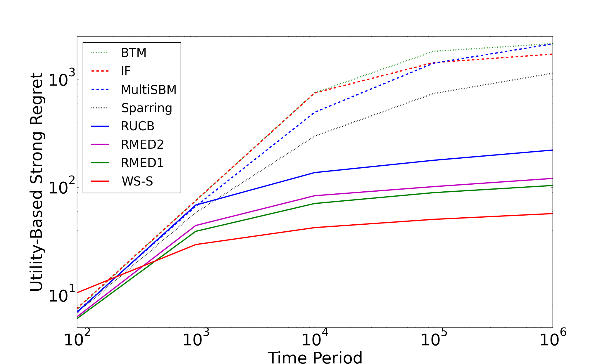
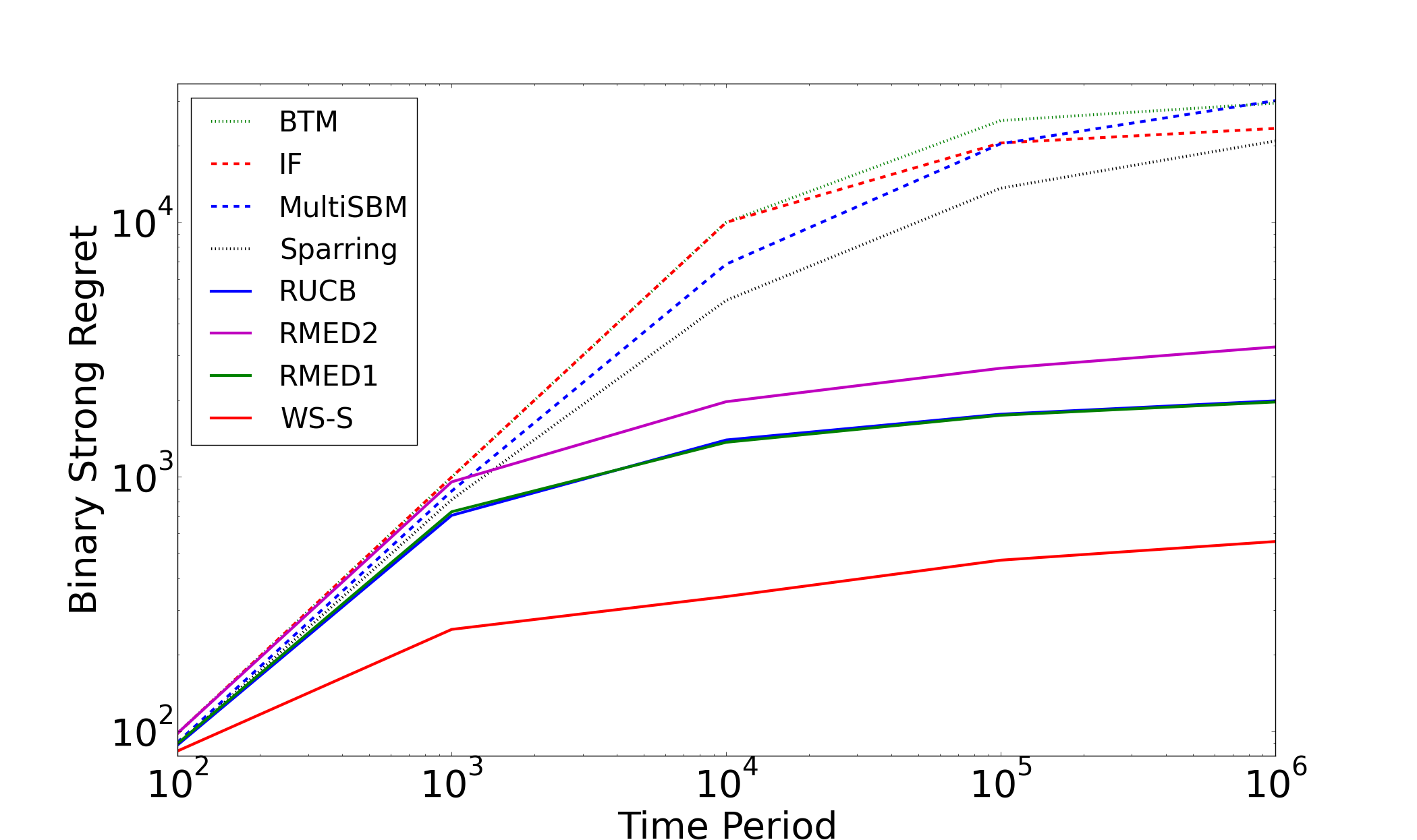
Again, we consider both binary strong regret and the utility-based strong regret. The utility-based strong regret is defined the same as the other two experiments. The result is summarized in Figure 5. WS-S outperforms all benchmarks considered in all time periods on binary regret, and outperforms them all in all time periods except on utility-based regret.
Appendix J Sensitivity Analysis
In this section, we conduct a sensitivity analysis of in WS-S using the MSLR dataset. In this analysis, we choose respectively and compare them with RMED and RUCB. The result is summarized in Figure 6.
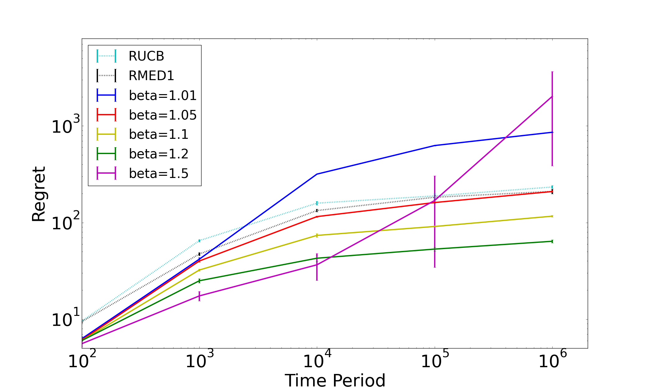
Based on Figure 6, WS-S with outperforms RMED and RUCB. When , we spend too much time on the exploration period and do not exploit enough. Similarly, WS-S with over exploits and does not explore enough. In both cases, WS-S underperforms RMED and RUCB. However, as long as is within a reasonable range, WS-S can outperform existing state-of-art algorithms.
langley00