$Z^{\prime}$ portal to Chern-Simons Dark Matter

arXiv: 1706.04198

Giorgio Arcadi Affiliation: Max Planck Institut für Kernphysik,
Saupfercheckweg 1, D-69117 Heidelberg, Germany Email: arcadi@mpi-hd.mpg.de Pradipta Ghosh Affiliation: Department of Physics, Vidyasagar College,
39, Sankar Ghosh Lane, Kolkata 700006, India Email: tphyspg@gmail.com Yann Mambrini Affiliation: Laboratoire de Physique Théorique, CNRS, Univ. Paris-Sud, Université Paris-Saclay,
91405 Orsay, France Email: yann.mambrini@th.u-psud.fr Mathias Pierre Affiliation: Laboratoire de Physique Théorique, CNRS, Univ. Paris-Sud, Université Paris-Saclay,
91405 Orsay, France Email: mathias.pierre@th.u-psud.fr Farinaldo S. Queiroz Affiliation: Max Planck Institut für Kernphysik,
Saupfercheckweg 1, D-69117 Heidelberg, Germany Email: queiroz@mpi-hd.mpg.de

Abstract

We study the phenomenological credibility of a vectorial dark matter, coupled to a $Z^{\prime}$ portal through Chern-Simons interaction. We scrutinize two possibilities of connecting a $Z^{\prime}$ with the Standard Model: (1) through kinetic mixing and (2) from a second Chern-Simons interaction. Both scenarios are characterized by suppressed nuclear recoil scatterings, rendering direct detection searches not promising. Indirect detection experiments, on the other hand, furnish complementary limits for TeV scale masses, specially with the CTA. Searches for mono-jet and dileptons signals at the LHC are important to partially probe the kinetic mixing setup. Finally we propose an UV completion of the Chern-Simons Dark Matter framework.

Keywords

dark matter theory, dark matter experiments

^†^†subheader: LPT-Orsay-17-28

1 Introduction

The nature of Dark Matter (DM) remains one of the most exciting and puzzling mysteries of science [1, 2, 3, 4, 5] till date. In the context of particle physics it is often assumed that one particle species can account for the entire DM abundance, which is $\sim$ 27% of the budget of the Universe as indicated by PLANCK [6]. Such a sizable amount of hitherto undetected matter has diverse and intricate consequences for various ongoing and near future direct and indirect DM detection experiments [7, 8, 9, 10, 11, 12, 13, 14, 15, 16, 17, 18, 19, 20].

The absence of conclusive signals of new physics beyond the Standard Model (SM) concerning the DM leaves a handful of open debate, e.g., what are the particle characteristics of the DM or how they are interacting with the SM particles. A popular solution for the DM puzzle is represented by the Weakly Interacting Massive Particles (WIMPs). In the simplest realization these new particle states, typically scalars or fermions, assumed to be singlet under the SM gauge group, feature interactions with the SM states mediated by the $Z$ or the SM-Higgs boson. Similar theoretical frameworks have also been addressed considering a vectorial DM [21, 22, 23, 24, 25, 26, 27, 28, 29, 30, 31, 32, 33]. Unfortunately, such simple models, except for a very few exceptions, are critically challenged by the existing and expected upcoming DM searches from the direct, indirect and collider probes. A detailed overview of these frameworks are addressed recently in ref. [34] (see also ref. [35]).

Considering apparent limitations of these simplest realizations, as extensively addressed in ref. [34], a natural extension of the above setup is provided by the so called “simplified models” (see ref. [36]) in which the SM mediators are replaced by a new “dark mediator”, of various spin assignations. This dark mediator can be connected to the SM particles by various ways and hence, relates the otherwise secluded DM to the SM particles. However, to ensure elucidate predictions, it is nevertheless necessary to investigate theoretical competence of these simplified setups [37, 38, 39, 40, 41], i.e., for example, whether they have consistent unitarity behaviours, reasonable Ultra-Violet (UV) completion and how they can be embedded into unified theory frameworks.

The case of spin-1 mediators, among these setups, perhaps deserves serious attentions as phenomenological study of these frameworks reveals intricate complementary aspects of DM searches with relevant collider observations (see ref. [34] for a thorough discussion). An intriguing origin of such spin-1 mediator(s) can arise as gauge boson(s) of some beyond the SM (BSM) gauge group(s), Abelian or non-Abelian, that simultaneously assigns non-zero gauge charge(s) also for the DM candidate. A spin-1 mediator, maintaining gauge invariance and renormalizability, can couple to the SM Electro-Weak (EW) gauge boson, and thus, subsequently to other SM particles, in a few different ways,¹¹ 1 A BSM spin-1 mediator can couple to the SM EW gauge bosons also via the well-known spontaneous symmetry breaking and Higgs mechanism, provided that the SM-Higgs doublet has non-zero charges under the BSM gauge groups. Spontaneous symmetry breaking in the BSM sector is triggered with new SM singlet scalar which may or may not mix with the SM-Higgs. We do not consider this possibility in our analysis. e.g., via a kinetic mixing²² 2 A kinetic mixing, from the principle of gauge invariance, is allowed only between the vector bosons of Abelian groups. [42, 43, 44, 45] or using a Chern-Simons (CS) interaction [46, 47, 48, 49]. The former can either appear naturally in Lagrangian preserving the gauge invariance and renormalizability of the SM [42, 44, 45] or can get generated after integrating out the heavy fermionic degrees of freedom [42, 43] charged under both the SM and BSM gauge groups. The latter can also arise in an analogous way after integrating out such heavy degrees of freedom, as extensively studied in ref. [50]. The presence of these new fermionic degrees of freedom, if chiral under some representations, introduces new challenges to construct an anomaly free model framework.³³ 3 One can always consider these new fermions to transform vector-like with respect to the SM gauge groups such that no new chiral anomalies appear in the SM. This goal is customarily achieved by arranging anomaly cancellation in the chiral sectors of the theory, by assigning specific couplings/charges for the involved particle species, e.g., by considering distinct couplings between the SM chiral fermions, and possibly also the DM, with the BSM spin-1 mediator as discussed in ref. [51] in the context of unified theories. Some classes of anomalies, like the triangle ones involving Abelian, non-Abelian or a mixture of the two gauge groups can, alternatively be cured through the Green-Schwarz mechanism [52, 53].

In this work we aim to study phenomenological viability of models, consisting of a vectorial DM candidate connected to the SM particles via a $Z^{\prime}$ -portal [54, 55, 56, 57, 58, 59, 60, 61, 62, 63, 64, 37, 65, 66, 67, 68, 38, 69, 70, 71, 69, 72, 73]. We consider specific frameworks that are inspired by Green-Schwarz mechanism (see also refs. [46, 48]), i.e., the connection between the DM and the $Z^{\prime}$ is mediated by a CS interaction. When considering theoretical arguments to account for the DM stability, for example an extended gauge structure, a vectorial DM candidate appears naturally and can be identified as the cosmologically stable gauge boson of a new BSM symmetry group provided that this gauge boson is the lightest state charged under this extra symmetry group while the $Z^{\prime}$ can arise from another BSM Abelian or non-Abelian gauge groups. CS interactions with $\mathcal{O}(1)$ couplings are possible by considering heavy chiral fermionic content charged under these extra gauge symmetry groups in an anomaly-free setup. This represents an intriguing possibility for DM phenomenology as both the DM candidate and its coupling to the $Z^{\prime}$ mediator would be a consequence of some extended gauge structure. Confining within the framework of Abelian theory, we will explore two possibilities of how a $Z^{\prime}$ can coordinate with the SM. These examples, as already mentioned, consider: (1) gauge invariant renormalizable kinetic mixing between the field strength of $Z^{\prime}$ with $B_{\mu\nu}$ , the SM hypercharge field strength and, (2) a second CS interaction involving $Z^{\prime}_{\mu}$ and the SM hypercharge vector $B_{\mu}$ . For both these scenarios we extensively investigate the impact of measured relic density [6] as well as the existing and anticipated sensitivity reaches from Direct Detection (DD) and Indirect Detection (ID) experiments on the associated model parameter spaces. In this setup we consider the vectorial DM candidate as a typical WIMP in a $\Lambda$ CDM cosmology [74, 6] and we further assume that the so called "small scale controversies" [75, 76, 77, 78, 79] to be unrelated and independent of the DM nature and properties.⁴⁴ 4 It has been recently pointed out that the baryonic feedback might alleviate existing tensions with N-body simulations (see e.g., refs. [80, 81, 82, 83, 84]). We also explore relevant theoretical constraints like EW Precision Tests (EWPTs), UV completion etc. for these setups. Finally, for completeness, we also discuss the possible pertinent collider aspects of such models, e.g., invisible $Z$ -decay width, mono-X, dijets, dilepton searches, etc.

The paper is organized as follows: in the next two sections we will study phenomenologies of the two aforesaid scenarios relying on the low-energy effective Lagrangians without specifying theoretical issues like UV completion etc. Section 4 will be dedicated for this task where we will address the generation of a CS coupling as well as a kinetic mixing in a UV complete setup. We will present the summary of our analyses and put our concluding remarks in section 5. Some useful formulae like detail constructions of an anomaly free model are relegated to the appendices.

2 Scenario-I: $Z^{\prime}$ - $Z$ interaction via kinetic mixing

In this section we study the aforesaid type-I scenario when the “dark sector”, comprised of a vectorial DM $X_{\mu}$ and a spin-1 vector boson $\widetilde{V}_{\mu}$ , is ‘‘secluded’’ from the visible sector, i.e., there exists no direct coupling between this dark sector and the SM fermions.⁵⁵ 5 The other possibility, i.e., the dark sector has direct couplings with the SM fermions is reviewed recently in ref. [34]. These $X_{\mu}$ and $\widetilde{V}_{\mu}$ , for example, can appear as the gauge bosons of some BSM $U(1)_{X}$ and $U(1)_{V}$ groups and we consider a CS interaction to connect them together. As already discussed, a bridge between the dark sector and the SM now appears via a kinetic mixing of $\widetilde{V}_{\mu\nu}$ and $B_{\mu\nu}$ , the field strengths associated with BSM $U(1)_{V}$ and the SM $U(1)_{Y}$ gauge group, respectively. A similar kinetic mixing between $X_{\mu\nu}$ and $B_{\mu\nu}$ , being renormalizable and allowed by the SM gauge invariance, should also be included in a general Lagrangian. However, we do not consider this possibility for the stability of the DM and postpone further discussion in this direction till section 4.

The relevant phenomenology of the said model can be described by the following low-energy effective Lagrangian:

	$\displaystyle\mathcal{L}\supset$		$\displaystyle-\frac{1}{4}{B}^{\mu\nu}{B}_{\mu\nu}-\frac{1}{4}X^{\mu\nu}X_{\mu\nu}-\frac{1}{4}\widetilde{V}^{\mu\nu}\widetilde{V}_{\mu\nu}-\frac{\sin\delta}{2}\widetilde{V}^{\mu\nu}{B}_{\mu\nu}$		(1)
			$\displaystyle+\alpha_{\rm CS}\epsilon^{\mu\nu\rho\sigma}X_{\mu}\widetilde{V}_{\nu}X_{\rho\sigma}+\dfrac{m_{V}^{2}}{2}\widetilde{V}^{\mu}\widetilde{V}_{\mu}+\dfrac{m_{X}^{2}}{2}X^{\mu}X_{\mu},$		(1)

here $\delta$ is the kinetic mixing parameter and $\alpha_{\rm CS}$ represents the effective coupling of CS operator. $X_{\mu\nu}$ gives the field strength of $U(1)_{X}$ group and $m_{V},\,m_{X}$ represent mass terms of the mediator and the DM. Thus, one gets a set of four free inputs, namely, $\delta,\,\alpha_{\rm CS}$ , $m_{V}$ and $m_{X}$ whose ranges will be tested subsequently imposing a series of theoretical and experimental constraints.

The presence of kinetic mixing in eq. (1) implies non-canonical kinetic term for $B_{\mu\nu}$ and also for $\widetilde{V}_{\mu\nu}$ . In order to generate diagonal kinetic terms in the physical or mass basis one should invoke three different rotations [85, 86, 87, 88]. The first rotation, involving then angle $\delta$ , takes $B_{\mu},\,\widetilde{V}_{\mu}$ to a basis (say $B^{\text{int}}_{\mu},\,\widetilde{V}^{\text{int}}_{\mu}$ ) with diagonal kinetic terms. The second rotation, after EW symmetry breaking (EWSB), via angle $\theta_{\widetilde{W}}$ , takes this $B^{\text{int}}_{\mu}$ together with $W^{3}_{\mu}$ to the intermediate $A_{\mu},\,Z^{\text{int}}_{\mu}$ basis. Finally, the third rotation through another angle $\phi$ , leaving the massless photon aside, takes $Z^{\text{int}}_{\mu},\,\widetilde{V}^{\text{int}}_{\mu}$ to the $Z_{\mu},\,Z^{\prime}_{\mu}$ basis where $Z_{\mu},\,Z^{\prime}_{\mu}$ are associated with the physical $Z$ and $Z^{\prime}$ boson. In summary, the initial $B_{\mu},\,W^{3}_{\mu},\,\widetilde{V}_{\mu}$ basis can be related to the physical $A_{\mu},\,Z_{\mu},\,Z^{\prime}_{\mu}$ basis in the following way:

\begin{bmatrix}{B}_{\mu}\\ W_{3\mu}\\ \widetilde{V}_{\mu}\end{bmatrix}=\begin{bmatrix}{c}_{\widetilde{W}}&-{s}_{\widetilde{W}}c_{\phi}+t_{\delta}s_{\phi}&-{s}_{\widetilde{W}}s_{\phi}-t_{\delta}c_{\phi}\\ {s}_{\widetilde{W}}&{c}_{\widetilde{W}}c_{\phi}&{c}_{\widetilde{W}}s_{\phi}\\ 0&-\dfrac{s_{\phi}}{c_{\delta}}&\dfrac{c_{\phi}}{c_{\delta}}\end{bmatrix}\begin{bmatrix}A_{\mu}\\ Z_{\mu}\\ Z^{\prime}_{\mu}\end{bmatrix},

(2)

where $t_{\delta},\,c_{\delta},\,c_{\widetilde{W}},\,s_{\widetilde{W}},\,s_{\phi},\,c_{\phi}\equiv\tan\delta,\,\cos\delta,\,\cos\theta_{\widetilde{W}},\,\sin\theta_{\widetilde{W}},\,\sin\phi,\,\cos\phi$ with:

\tan 2\phi=\dfrac{\widetilde{m}_{Z}^{2}{s}_{\widetilde{W}}\sin 2\delta}{m_{V}^{2}-\widetilde{m}_{Z}^{2}(c_{\delta}^{2}-{s^{2}}_{\widetilde{W}}s_{\delta}^{2})},

(3)

here $s_{\delta}\equiv\sin\delta$ . The quantities $\theta_{\widetilde{W}},\,\widetilde{m}_{Z}$ do not represent the measured values of Weinberg angle and $Z$ -boson mass [89] but are related to them as will be explained later. These quantities are obtained after the SM EWSB using a rotated $B_{\mu}$ field (a basis where off-diagonal mixing term of eq. (1) between $B_{\mu}$ and $\widetilde{V}_{\mu}$ vanishes) and the $W^{3}_{\mu}$ field of the SM. The masses of $Z^{\prime}$ and $Z$ are written as:

m_{Z^{\prime},Z}^{2}=\dfrac{1}{2}\left[\widetilde{m}_{Z}^{2}(1+{s^{2}}_{\widetilde{W}}t_{\delta}^{2})+\dfrac{m_{V}^{2}}{c_{\delta}^{2}}\pm\sqrt{(\widetilde{m}_{Z}^{2}(1+{s^{2}}_{\widetilde{W}}t_{\delta}^{2})+\dfrac{m_{V}^{2}}{c_{\delta}^{2}})^{2}-\dfrac{4}{c_{\delta}^{2}}\widetilde{m}_{Z}^{2}m_{V}^{2}}\right],

(4)

which gives $m_{Z}\simeq\widetilde{m}_{Z}$ in the experimentally favoured limit $\delta\ll 1$ , along with $m_{Z^{\prime}}\simeq m_{V}$ .

Notice that the transformation used in eq. (2) is valid only if one of these two conditions is met:

	$\displaystyle\frac{m_{V}^{2}}{\widetilde{m}_{Z}^{2}}$		$\displaystyle\geq 1+2s_{\widetilde{W}}\tan^{2}\delta+2\sqrt{s_{\widetilde{W}}^{2}\tan^{2}\delta\left(1+s_{\widetilde{W}}^{2}\tan^{2}\delta\right)},$
	$\displaystyle\frac{m_{V}^{2}}{\widetilde{m}_{Z}^{2}}$		$\displaystyle\leq 1+2s_{\widetilde{W}}\tan^{2}\delta-2\sqrt{s_{\widetilde{W}}^{2}\tan^{2}\delta\left(1+s_{\widetilde{W}}^{2}\tan^{2}\delta\right)}.$		(5)

One should note that the transformation of eq. (2) does not change the photon coupling [85], implying the following identity:

s_{\widetilde{W}}c_{\widetilde{W}}\widetilde{m}_{Z}^{2}=s_{W}c_{W}m_{Z}^{2}=\frac{\pi\alpha(m_{Z})}{\sqrt{2}G_{F}},

(6)

where $s_{W},\,c_{W}\equiv\sin\theta_{W},\,\cos\theta_{W}$ are associated with the measured value of Weinberg angle $\theta_{W}$ [89]. $\alpha(m_{Z})$ is the fine structure constant at the energy scale $m_{Z}$ and $G_{F}$ represents the Fermi constant [89].

One should also consider the invariance of $W$ -boson mass under the transformation of eq. (2), i.e., $m_{W}^{2}=m^{2}_{Z}c_{W}^{2}=\widetilde{m}_{Z}^{2}{c^{2}}_{\widetilde{W}}$ which allows us to express the $\rho$ parameter [89] as:

\rho=\frac{\widetilde{m}_{Z}^{2}{c^{2}}_{\widetilde{W}}}{m^{2}_{Z}c^{2}_{W}},

(7)

with the experimental measured value given by $\rho-1=4^{+8}_{-4}\times 10^{-4}$ [89]. Further, from the EWPT one can consider a simple and conservative limit on $\delta$ as [90, 91, 92, 86]:

\delta\lesssim\arctan\left[0.4\left(\dfrac{m_{Z^{\prime}}}{\text{TeV}}\right)\right].

(8)

It is now apparent that one can use eq. (6), eq. (7) and eq. (8) to discard experimentally disfavoured values of the kinetic mixing parameter $\delta$ . Further constraints on $\delta$ can emerge from various other experimental observations. The mixing among $B_{\mu},\,W^{3}_{\mu}$ and $\widetilde{V}_{\mu}$ (see eq. (2)), couples the SM fermions and the DM with the $Z$ boson. The latter coupling implies an enhancement of the invisible $Z$ decay width for $2m_{X}<m_{Z}$ . Hence, the parameter $\delta$ , along with $m_{V}$ , will receive constraints from a plethora of different collider searches like dileptons $(pp\to Z^{\prime}$ $\to e^{+}e^{-}$ , $\mu^{+}\mu^{-})$ [93, 94, 95], dijets $(pp\to Z^{\prime}\to q\overline{q})$ [96, 97, 98, 99], mono-X $(pp\to Z^{\prime}+{\mathbf{X}},\,Z^{\prime}\to{\rm DM\penalty\ pairs})$ with ${\mathbf{X}}=q/g$ [100], $W$ [101], $Z$ [101, 102], $\gamma$ [103, 104, 105], SM-Higgs [106, 107, 108], etc., invisible $Z$ decay width [89] and a few others. The dijets and mono-X searches also restrict the parameters $\alpha_{\rm CS},\,m_{X}$ . Finally, the DM phenomenology, i.e., the correct relic density, DD and ID results will also put limits on the parameters $\delta,\,\alpha_{\rm CS},\,m_{V}$ and $m_{X}$ . We note in passing that for numerical analyses we have traded the parameter $m_{V}$ with the physical mass $m_{Z^{\prime}}$ using eq. (4).

In the mass basis, the Lagrangian relevant for our subsequent analysis is given by:

$\displaystyle\mathcal{L}_{Z/Z^{\prime},SM}$	$\displaystyle=\overline{f}\gamma^{\mu}\left(g_{f_{L}}^{Z}P_{L}+g_{f_{R}}^{Z}P_{R}\right)fZ_{\mu}+\overline{f}\gamma^{\mu}\left(g_{f_{L}}^{Z^{\prime}}P_{L}+g_{f_{R}}^{Z^{\prime}}P_{R}\right)fZ^{\prime}_{\mu}$	(9)
	$\displaystyle+g_{W}^{Z}[[W^{+}W^{-}Z]]+g_{W}^{Z^{\prime}}[[W^{+}W^{-}Z^{\prime}]]+\dfrac{g_{hZZ}}{2}Z^{\mu}Z_{\mu}h+g_{hZZ^{\prime}}Z^{\prime}_{\mu}Z^{\mu}h$
	$\displaystyle+\dfrac{g_{hZ^{\prime}Z^{\prime}}}{2}Z^{\prime}_{\mu}Z^{\prime\mu}h-\alpha_{\rm CS}\,\frac{s_{\phi}}{c_{\delta}}\,\epsilon^{\mu\nu\rho\sigma}\,X_{\mu}X_{\rho\sigma}Z_{\nu}+\alpha_{\rm CS}\,\frac{c_{\phi}}{c_{\delta}}\,\epsilon^{\mu\nu\rho\sigma}\,X_{\mu}X_{\rho\sigma}Z^{{}^{\prime}}_{\nu},$

here $P_{L(R)}=(1\pm\gamma_{5})/2$ and

	$\displaystyle g^{Z}_{f_{L}}$		$\displaystyle=g_{Y}Y_{L}(-s_{W}c_{\phi}+t_{\delta}s_{\phi})+g_{W}I_{z}(c_{W}c_{\phi}),\,\,\,\,g^{Z}_{f_{R}}=g_{Y}Y_{R}(-s_{W}c_{\phi}+t_{\delta}s_{\phi}),$
	$\displaystyle g^{Z^{\prime}}_{f_{L}}$		$\displaystyle=g_{Y}Y_{L}(-s_{W}s_{\phi}-t_{\delta}c_{\phi})+g_{W}I_{z}(c_{W}s_{\phi}),\,\,\,\,g^{Z^{\prime}}_{f_{R}}=g_{Y}Y_{R}(-s_{W}s_{\phi}-t_{\delta}c_{\phi}),$		(10)

where $g_{Y}$ is the gauge coupling of $U(1)_{Y}$ , $I_{z}$ is the $3^{rd}$ component of the weak isospin, $Y_{L,R}$ are hypercharge of the left- and right- chiral fermions, $g_{W}$ is the $SU(2)_{L}$ gauge coupling.

g^{Z}_{W}=g_{W}c_{W}c_{\phi},\,\,\,\qquad g^{Z^{\prime}}_{W}=g_{W}c_{W}s_{\phi},

(11)

$\displaystyle g_{hZZ}$	$\displaystyle=2v_{h}\Big[\frac{g_{Y}}{2}(-s_{W}c_{\phi}+t_{\delta}s_{\phi})-\frac{g_{W}}{2}(c_{W}c_{\phi})\Big]^{2},$
$\displaystyle g_{hZZ^{\prime}}$	$\displaystyle=2v_{h}\Big[\frac{g_{Y}}{2}(-s_{W}s_{\phi}-t_{\delta}c_{\phi})-\frac{g_{W}}{2}(c_{W}s_{\phi})\Big]\Big[\frac{g_{Y}}{2}(-s_{W}c_{\phi}+t_{\delta}s_{\phi})-\frac{g_{W}}{2}(c_{W}c_{\phi})\Big],$
$\displaystyle g_{hZ^{\prime}Z^{\prime}}$	$\displaystyle=2v_{h}\Big[\frac{g_{Y}}{2}(-s_{W}s_{\phi}-t_{\delta}c_{\phi})-\frac{g_{W}}{2}(c_{W}s_{\phi})\Big]^{2},$	(12)

here $v_{h}$ is the vacuum expectation value (VEV) of the SM-Higgs doublet and a factor ‘ $2$ ’ appears in $ZZh,\,Z^{\prime}Z^{\prime}h$ vertices due to the presence of identical particles. For the $\alpha_{\rm CS}\,\frac{-s_{\phi}(c_{\phi})}{c_{\delta}}$ $\epsilon^{\mu\nu\rho\sigma}$ $X_{\mu}X_{\rho\sigma}Z_{\nu}(Z^{{}^{\prime}}_{\nu})$ term, considering the following momentum assignments $X_{\mu}(p_{a})X_{\nu}(p_{b})$ $Z_{\rho}/Z^{\prime}_{\rho}$ one can use

g_{X}^{Z}=-2\alpha_{\rm CS}\,\frac{s_{\phi}}{c_{\delta}},\,\,\,\,g^{Z^{\prime}}_{X}=2\alpha_{\rm CS}\,\frac{c_{\phi}}{c_{\delta}},

(13)

for subsequent relevant analytical formulae like DM pair annihilation cross-section etc. Once again the factor ‘ $2$ ’ appears due to identical particles. Lastly

	$\displaystyle[[W^{+}W^{-}Z(Z^{\prime})]]$		$\displaystyle\equiv i\left[W^{+}_{\mu\nu}W^{-\,\mu}Z(Z^{\prime})^{\nu}-W^{+}_{\,\mu\nu}W^{-\,\mu}Z(Z^{\prime})^{\nu}\right.$		(14)
			$\displaystyle\left.\penalty\ \penalty\ \penalty\ \penalty\ +\frac{1}{2}Z(Z^{\prime})^{\mu\nu}\left(W^{+}_{\mu}W^{-}_{\nu}-W^{+}_{\nu}W^{-}_{\mu}\right)\right].$		(14)

With these analytical expressions now we will discuss the DM phenomenology of this framework in the next subsection.

2.1 Dark Matter Phenomenology

In this subsection we discuss the DM phenomenology in the light of various constraints coming from the requirement of correct relic density and consistency with the existing and/or upcoming DD and ID results. The DM is produced in the early Universe according to the WIMP paradigm. We will subsequently discuss how these observations can affect the accessibility of the chosen set-up at the present or in the near future DM detection experiments, assuming projected search sensitivities. Nevertheless, for the sake of completeness, we will also qualitatively discuss the complementary limits arising from the EWPT, collider searches, etc. We start our discussion in the context of accommodating correct relic density and successively will address the restrictions coming from direct and indirect DM searches.

2.1.1 Relic density

It is well known that according to the WIMP paradigm a single particle species can account for the correct DM relic density $\Omega_{X}h^{2}$ $\propto 1/\langle\sigma v\rangle$ , where $\langle\sigma v\rangle$ represents the thermally averaged DM pair annihilation cross-section into the SM states. The experimentally hinted value $\Omega_{X}h^{2}\approx 0.12$ [6] predicts $\langle\sigma v\rangle$ , $\sim\mathcal{O}$ $(10^{-26}\,{\mbox{cm}}^{3}\,{\mbox{s}}^{-1})$ .

In the chosen framework (see Section 2), the DM pair can annihilate into the SM fermions $(\overline{f}f)$ and $W^{+}W^{-}$ , as well as in $Zh$ and $Z^{\prime}h$ final states, through s-channel exchange of the $Z/Z^{\prime}$ boson, and into $ZZ,\,ZZ^{\prime}$ and $Z^{\prime}Z^{\prime}$ final states, through t-channel exchange of a DM state. Approximate analytical expressions of the corresponding annihilation cross-sections are obtained through the expansion $\langle\sigma v\rangle\simeq a+b\dfrac{1}{x}+...$ with $x=\dfrac{m_{X}}{T}$ [109, 110], $T$ being the temperature. We remind, however, that the aforesaid approximation is not reliable over the entire parameter space [111], e.g., the pole regions $m_{X}\sim\dfrac{m_{Z,\,Z^{\prime}}}{2}$ . Hence, all results presented in this article are obtained through full numerical computations using the package micrOMEGAs [112, 113, 114], after implementing the model in FeynRules [115, 116]. The DM annihilation cross-sections in the possible final states are given as:

•

$XX\to\overline{f}f:$

	$\displaystyle\langle\sigma v\rangle_{\bar{f}f}$		$\displaystyle\simeq\frac{n_{c}\,m_{f}^{2}}{3\pi}\sqrt{1-\frac{m_{f}^{2}}{m_{X}^{2}}}{\left(\frac{\left(g_{f_{L}}^{Z}-g_{f_{R}}^{Z}\right)g_{X}^{Z}}{m_{Z}^{2}}+\frac{\left(g_{f_{L}}^{Z^{\prime}}-g_{f_{R}}^{Z^{\prime}}\right)g_{X}^{Z^{\prime}}}{m_{Z^{\prime}}^{2}}\right)}^{2}\dfrac{1}{x}$		(15)
			$\displaystyle+\frac{n_{c}}{108\pi}\left[{\left(\frac{g^{Z}_{X}g^{Z}_{f_{L}}}{m^{2}_{Z}}+\frac{g^{Z^{\prime}}_{X}g^{Z^{\prime}}_{f_{L}}}{m^{2}_{Z^{\prime}}}\right)}^{2}+{\left(\frac{g^{Z}_{X}g^{Z}_{f_{R}}}{m^{2}_{Z}}+\frac{g^{Z^{\prime}}_{X}g^{Z^{\prime}}_{f_{R}}}{m^{2}_{Z^{\prime}}}\right)}^{2}\right]\frac{1}{x^{2}}$		(15)

where we have written not only the leading $1/x$ (p-wave) term but also the second order $1/x^{2}$ (d-wave) one which appears to be the dominant one since the first one is suppressed by the square of SM fermion mass $m^{2}_{f}$ . The parameter $n_{c}$ denotes colour factor with a value of $3\,(1)$ for quarks (leptons).

•

$XX\to W^{+}W^{-}:$

\langle\sigma v\rangle_{W^{+}W^{-}}\simeq\frac{5}{9\pi m_{W}^{4}}{\left(\frac{g_{X}^{Z}g_{W}^{Z}m_{X}}{4}-\frac{g_{X}^{Z^{\prime}}g_{W}^{Z^{\prime}}m_{X}^{3}}{m_{Z^{\prime}}^{2}}\right)}^{2}\dfrac{1}{x^{2}},\penalty\ \penalty\ {\rm for\penalty\ }m_{W,\,Z}\ll m_{X}\ll m_{Z^{\prime}}.

(16)

•

$XX\to Zh:$

\langle\sigma v\rangle_{Zh}\simeq\frac{2}{3\pi}\frac{m_{X}^{6}}{m_{Z}^{6}}{\left(\frac{g_{X}^{Z}g_{hZZ}}{4m_{X}^{2}}-\frac{g_{X}^{Z^{\prime}}g_{hZZ^{\prime}}}{m_{Z^{\prime}}^{2}}\right)}^{2}\dfrac{1}{x},\penalty\ \penalty\ {\rm for\penalty\ }m_{Z}\sim m_{h}\ll m_{X}\ll m_{Z^{\prime}}.

(17)

•

$XX\to Z^{\prime}h:$

\langle\sigma v\rangle_{Z^{\prime}h}\simeq\frac{1}{24\pi}\frac{m_{X}^{2}}{m_{Z^{\prime}}^{6}}{\left(g_{hZZ^{\prime}}g_{X}^{Z}+g_{hZ^{\prime}Z^{\prime}}g_{X}^{Z^{\prime}}\right)}^{2}\dfrac{1}{x},\penalty\ \penalty\ {\rm for\penalty\ }m_{Z}\sim m_{h}\ll m_{Z^{\prime}}\ll m_{X}.

(18)

•

$XX\to ZZ:$

\langle\sigma v\rangle_{ZZ}\simeq\frac{8\alpha_{\rm CS}^{4}\delta^{4}m_{X}^{2}m_{Z}^{4}s_{W}^{4}}{9\pi m_{Z^{\prime}}^{8}},\penalty\ \penalty\ {\rm for\penalty\ }m_{Z}\ll m_{X}\ll m_{Z^{\prime}}.

(19)

•

$XX\to Z^{\prime}Z^{\prime}:$

\langle\sigma v\rangle_{Z^{\prime}Z^{\prime}}\simeq\frac{8\alpha_{\rm CS}^{4}m_{X}^{2}}{9\pi m_{Z^{\prime}}^{4}},\penalty\ \penalty\ {\rm for\penalty\ }m_{Z}\ll m_{Z^{\prime}}\ll m_{X}.

(20)

•

$XX\to Z^{\prime}Z:$

\langle\sigma v\rangle_{Z^{\prime}Z}\simeq\frac{16\alpha_{\rm CS}^{4}\delta^{2}m_{X}^{2}m_{Z}^{2}s_{W}^{2}}{9\pi m_{Z^{\prime}}^{6}},\penalty\ \penalty\ {\rm for\penalty\ }m_{Z}\ll m_{Z^{\prime}}\ll m_{X}.

(21)

As evident from the above expressions that annihilation channels originated by s-channel exchange of the $Z/Z^{\prime}$ feature a suppressed annihilation cross-section, at least p-wave or even d-wave in the cases of $W^{+}W^{-}$ and $\overline{f}f$ final states (see eq. (16) and eq. (15)). For the latter a p-wave contribution is also present but it is helicity suppressed. The t-channel induced annihilations feature, instead, a s-wave cross-section. The cross-section into $ZZ$ pairs (see eq. (19)) is anyway suppressed by an higher power of the kinetic mixing parameter $\delta$ , with respect to the other annihilation channels.

The DM pair annihilation cross-section, as depicted in figure 1, typically lies much below the thermally favoured value, i.e., $10^{-{26}}\,{\rm cm}^{3}\,{\rm s}^{-1}$ , ad exception of the pole regions $m_{X}\sim m_{Z}/2,m_{Z^{\prime}}/2$ , or DM masses above several hundreds of GeV so that at least annihilations into $ZZ^{\prime}$ final state appears kinematically accessible.

Figure 1: Variation of the thermally averaged DM pair annihilation cross-section

\langle\sigma v\rangle

, at thermal freeze-out, as function of the DM mass

m_{X}

for

m_{Z^{\prime}}=400

GeV (left) and

800

GeV (right) with two values of

\alpha_{\rm CS}=0.1

(red coloured solid line) and

0.5

(orange coloured solid line) keeping kinetic mixing parameter

\delta=0.1

. The black coloured dashed line represents the thermally favoured value of

\langle\sigma v\rangle=

3\times 10^{-26}\,{\mbox{cm}}^{3}\,{\mbox{s}}^{-1}

. The magenta coloured region with dashed outline represents the resultant exclusion from the combined FERMI-LAT and MAGIC observations (abbreviated as FERMI-MAGIC in all the successive relevant figures) while the blue coloured region with dashed boundary represents the region already excluded by HESS for a Einasto density profile of the DM. Finally, the purple colour region with dashed outline represents the expected future exclusion from CTA.

2.1.2 Indirect detection

Residual annihilation processes of the DM at the present times could be efficient enough so that they might be detected by the Earth based telescopes or satellites. The absence of definite signals till date are translated into upper bounds on $\langle\sigma v\rangle$ as a function of the DM mass. At the moment, the strongest limits come from searches of the gamma-rays produced in the DM annihilations. For DM masses below a few hundred GeVs, these limits are set by the FERMI satellite [117] and exclude the thermally favoured values of $\langle\sigma v\rangle$ for $m_{X}<100$ GeV. For higher values of $m_{X}$ the best sensitivity is achieved by HESS [118] which has put a limit $\langle\sigma v\rangle\lesssim 10^{-25}\text{cm}^{3}\,\text{s}^{-1}$ for $m_{X}\sim 1\,{\mbox{TeV}}$ , considering a Einasto density profile for the DM.

As shown earlier while discussing the relic density that most of the DM annihilation processes have a p-wave (or even d-wave) annihilation cross-section, i.e., they are velocity dependent. As a consequence the DM annihilation at present times is suppressed by several orders of magnitude with respect to its value at the thermal freeze-out and thus, limits from DM ID are actually not effective. ID can probe the WIMP paradigm for the DM relic density only when the latter is mostly determined by processes with an s-wave (i.e., velocity independent) annihilation cross-section. In our setup this requirement is fulfilled by annihilation into $Z^{\prime}Z$ and $Z^{\prime}Z^{\prime}$ states (see eq. (21) and eq. (20)). The other s-wave dominated annihilation into $ZZ$ final state (see eq. (19)), as already addressed, is insignificant as it is suppressed by the fourth power of kinetic mixing parameter $\delta$ .

We have thus compared the DM annihilation cross-section into $Z^{\prime}Z$ and $Z^{\prime}Z^{\prime}$ final states with the limits derived from combined analysis of the MAGIC and FERMI-LAT observations (abbreviated as FERMI-MAGIC) of the dwarf spheroidal galaxies (dSphs) [119]. We also consider limits from $10$ years of observations towards the inner galactic halo by HESS [120]. In the absence of a dedicated analysis for the considered final states we have applied the limit for gamma-rays originating from $W^{+}W^{-}$ pairs. This choice is reasonable since the $Z^{\prime}$ decays efficiently into hadrons as the SM gauge bosons. Any mild change in the limits as a result of this assumption is beyond the scope of our current work.

Our results are reported in figure 1 concerning changes of the DM pair annihilation cross-section at thermal freeze-out with the DM mass $m_{X}$ , for specific assignations of the other relevant inputs, detailed in the figure caption. As evident from this figure that the impact of ID limits from FERMI-MAGIC (magenta coloured region) and HESS (blue coloured region) appears to be rather limited. This can be understood by looking at this simple analytical estimate for $\langle\sigma v\rangle_{Z^{\prime}Z^{\prime}}$ :

\langle\sigma v\rangle_{Z^{\prime}Z^{\prime}}\simeq\dfrac{8\alpha_{\text{CS}}^{4}m_{X}^{2}}{9\pi m_{Z^{\prime}}^{4}}\simeq 3\times 10^{-28}\text{cm}^{3}\,\text{s}^{-1}\Big(\dfrac{\alpha_{\text{CS}}}{0.1}\Big)^{4}\Big(\dfrac{m_{X}}{1\text{ TeV}}\Big)^{2}\Big(\dfrac{m_{Z^{\prime}}}{1\text{ TeV}}\Big)^{-4},

(22)

which shows that a value of the cross-section equal or bigger than the thermal expectation i.e., $\sim\mathcal{O}(10^{-26}\,\text{cm}^{3}\,\text{s}^{-1})$ , can be achieved only for masses of the $Z^{\prime}$ not exceeding a few hundreds of GeV and/or $\alpha_{\rm CS}\sim 0.5$ . Such value of $\alpha_{\rm CS}$ , however, is somewhat extreme since this coupling is expected to have a radiative origin as will be discussed later. The impact of possible limits from ID will be anyway increased in the near future by Cherenkov Telescope Array a.k.a. CTA [121, 122, 123, 124, 125, 126] which we have reported (purple coloured region) in figure 1, assuming a projected limits from $500$ h of observation towards the galactic center.

2.1.3 Direct detection

DD experiments aim at measuring the recoil energy released by an atomic nuclei upon a scattering process with a DM state. Several experiments have performed searches for DM scattering off nuclei reaching, in the last year, an impressive sensitivity. In particular, in the case of Spin Independent (SI) interactions of the DM with nuclei, a cross-section $\sim\mathcal{O}(10^{-46}\text{ cm}^{2})$ , for DM mass of $50$ GeV, has been excluded by the LUX [127] and PandaX [128]. These experiments play also a leading role in constraining the Spin Dependent (SD) interactions. In this case the maximal sensitivity is achieved for DM mass of $40$ GeV which corresponds to a value $\sim 10^{-41}\text{ cm}^{2}$ of the DM-nucleon scattering cross-section [129].

In the chosen setup (see eq. (1)), scattering of the DM with nucleons is originated, at the microscopic level, by an interaction between the DM and the SM quarks mediated via t-channel exchange of the $Z/Z^{\prime}$ boson. An interaction of this kind, in the non-relativistic limit, is described by the following effective operator [113]:

\mathcal{L}_{\rm DM\penalty\ scattering}=\left(\frac{g_{X}^{Z}a_{q}^{Z}}{m_{Z}^{2}}+\frac{g_{X}^{Z^{\prime}}a_{q}^{Z^{\prime}}}{m_{Z^{\prime}}^{2}}\right)\left(\partial_{\alpha}X_{\beta}X_{\nu}-X_{\beta}\partial_{\alpha}X_{\nu}\right)\epsilon^{\alpha\beta\nu\mu}\overline{q}\gamma_{\mu}\gamma_{5}q,

(23)

where $a_{q}^{Z^{\prime}}=\dfrac{g^{Z^{\prime}}_{q_{R}}-g^{Z^{\prime}}_{q_{L}}}{2}$ and $a_{q}^{Z}=\dfrac{g^{Z}_{q_{R}}-g^{Z}_{q_{L}}}{2}$ , which corresponds to a SD interaction with squared amplitude:

\overline{|\mathcal{M}|^{2}}=\dfrac{32m^{2}_{X}m^{2}_{N}}{m^{4}_{Z}m^{4}_{Z^{\prime}}}\Big(\sum_{q}a^{Z}_{q}\Delta_{q}^{N}g_{X}^{Z}m_{Z^{\prime}}^{2}+\sum_{q}a^{Z^{\prime}}_{q}\Delta_{q}^{N}g_{X}^{Z^{\prime}}m_{Z}^{2}\Big)^{2},

(24)

with $m_{N}$ denoting the mass of a nucleon $N=p,\,n$ while $\Delta_{q}^{N}$ represents the contribution of the quark $q$ to the spin of the nucleon $N$ . The SD scattering cross-section can be straightforwardly derived, taking into account the multiple isotopes present in the detector material as:

\sigma_{Xp}^{\text{SD}}=\dfrac{2}{\pi}\dfrac{\mu^{2}_{Xp}}{m_{Z}^{4}m_{Z^{\prime}}^{4}}\frac{\sum\limits_{A}\eta_{A}\Big(S^{A}_{Z}g_{X}^{Z}m_{Z^{\prime}}^{2}+S^{A}_{Z^{\prime}}g_{X}^{Z^{\prime}}m_{Z}^{2}\Big)^{2}}{\sum\limits_{A}\eta_{A}\Big(S^{A}_{n}+S^{A}_{p}\Big)^{2}},

(25)

where $\mu_{Xp}=m_{X}m_{p}/(m_{X}+m_{p})$ is the reduced mass for the DM-proton system and $S^{A}_{Z^{(\prime)}}=a^{Z^{(\prime)}}_{u}(\Delta^{p}_{u}S^{A}_{p}+\Delta^{p}_{d}S^{A}_{n})+a^{Z^{(\prime)}}_{d}[(\Delta^{p}_{d}+\Delta^{p}_{s})S^{A}_{p}+(\Delta^{p}_{u}+\Delta^{p}_{s})S^{A}_{n}]$ . Here $S^{A}_{p,n}$ represents the contribution of protons and neutrons to the spin of a nucleus with atomic number $A$ while $\eta_{A}$ represents the relative abundance of a given isotope of the element constituting the target material. Notice that the result is almost independent of the DM mass since the only dependence through $\mu_{Xp}$ will vanish for $m_{X}\gg m_{p}$ giving $\mu_{Xp}\sim m_{p}$ . A simple estimate of $\sigma_{Xp}^{\text{SD}}$ can be performed assuming $\delta,\alpha_{\text{CS}}\ll 1$ as:

\sigma_{Xp}^{\text{SD}}\simeq 6\times 10^{-50}\text{cm}^{2}\Big(\dfrac{\delta}{0.1}\Big)^{2}\Big(\dfrac{\alpha_{\text{CS}}}{0.1}\Big)^{2}\Big(\dfrac{m_{Z^{\prime}}}{1\text{ TeV}}\Big)^{-4},

(26)

which gives values of $\sigma_{Xp}^{\text{SD}}$ well below the current maximal sensitivity ( $10^{-41}\text{cm}^{2}$ ), and remains also beyond the reach of next generation detectors for the chosen set of parameter values, consistent with other existing constraints.

2.2 Collider phenomenology

Phenomenological models, where the DM candidate interacts with the SM fields through a spin-1 mediator typically posses a rich collider phenomenology. In the case when on-shell production of a $Z^{\prime}$ is kinematically accessible in proton-proton collision, detectable signals can appear from the decays of $Z^{\prime}$ into SM fermions, showing a new resonance in the invariant mass distribution of dijets [96, 97, 98, 99] or dileptons [93, 94, 95] as well as from possible decay of a $Z^{\prime}$ into DM pairs which can be probed through mono-X searches (X= hadronic jets, photon, weak gauge bosons, SM-Higgs) [100, 101, 102, 103, 104, 105, 106, 107, 108] accompanied by moderate/large missing transverse energy/momentum. Interestingly, the relative relevance of these two kinds of searches, i.e., resonances and mono-X events, is mainly set by the invisible decay branching fraction (Br) of the $Z^{\prime}$ which, in turn, is constrained by the DM observables that primarily appears from the requirement of correct relic density for the chosen framework.

Refer to caption — Figure 2: Comparison of the production cross-sections for $pp\to Z^{\prime}\to jj$ (left panel) and $pp\to Z^{\prime}\to l^{+}l^{-}$ (right panel) processes for an on-shell $Z^{\prime}$ in the chosen theory framework with the relevant experimental limits [96] and [95], respectively, as a function of $m_{Z^{\prime}}$ for three fixed values of $\delta=10^{-3},\,10^{-2}$ and $10^{-1}$ . Here the solid red coloured curve represents the observed experimental limit while dashed black coloured line, green and yellow coloured bands represent the expected limit and its $1\sigma,\,2\sigma$ ranges. The dotted purple, red and dashed orange coloured lines are used for $\delta=0.001,\,0.01$ and $0.1$ configurations, respectively. For simplicity, we have considered the case of $2m_{X}>m_{Z^{\prime}}$ so that $Z^{\prime}$ has only visible decays. In our analysis we consider $j=u,\,d,\,c,\,s,\,b$ and $t$ for $m_{Z^{\prime}}>2m_{t}$ and $l=e,\,\mu$ .

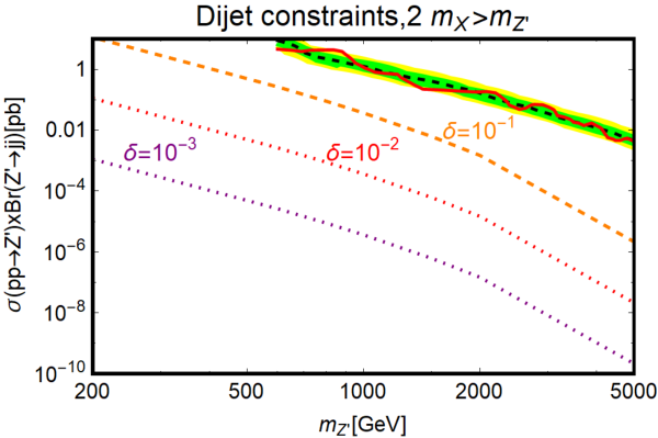
The impact of experimental limits from resonance searches is depicted in figure 2 where, for simplicity, we consider $2m_{X}>m_{Z^{\prime}}$ to forbid $Z^{\prime}\to$ DM pairs process. For these analyses we consider all possible quark flavours including top for $m_{Z^{\prime}}>2m_{t}$ regime while $l=e$ and $\mu$ only. Here we have compared the results of numerical simulations for the chosen setup with the experimental ones including $1\sigma,\,2\sigma$ variations of the production cross-sections as observed in refs. [96] and [95], respectively. Since the $Z^{\prime}$ -SM fermions mixing (see eq. (10)) appears from an effective $Z$ - $Z^{\prime}$ mixing, both $\sigma(pp\to Z^{\prime})$ and Br( $Z\to jj/l^{+}l^{-}$ ) are sensitive to the parameter $\delta$ . The resultant $\delta^{2}$ dependence thus, hints diminishing $\sigma(pp\to Z^{\prime})\times{\rm Br}(Z^{\prime}\to jj/l^{+}l^{-})$ values for decreasing $\delta$ values, as also reflected in figure 2. It is evident from figure 2 that once values of the kinetic mixing parameter $\delta$ smaller than $\mathcal{O}(1)$ are considered to comply with the theoretical and EWPT (see eq. (8)) constraints, only the limits from dileptons resonance searches remain effective. For $\delta=0.1$ , values of $m_{Z^{\prime}}$ below 2 TeV are ruled out while for $\delta=0.01$ , a much weaker lower bound of approximately 300 GeV is obtained on $m_{Z^{\prime}}$ . For further lower values of $\delta$ , very small $\delta^{2}$ dependence⁶⁶ 6 Holds true for a resonant production with no/suppressed invisible decay of $Z^{\prime}$ . makes $m_{Z^{\prime}}$ unconstrained from the aforesaid searches.

In the presence of a non-zero and sizable invisible branching fraction for $Z^{\prime}$ , i.e., Br( $Z^{\prime}\to$ DM pairs), the production cross-sections of dijets/dileptons get suppressed by the enhanced decay width of $Z^{\prime}$ . In such a scenario, the cross-section corresponding to mono-X signals might become sizable, possibly providing complementary constraints. We preserve the discussion of such complementary signals for the next subsection.

2.3 Results

In this subsection we report the impact of various constraints, as mentioned in the previous subsections, on the parameter space of the model. As already pointed out the effect of DD and ID constraints on our model framework is substantially negligible. Concerning the DM phenomenology, the only relevant constraint comes from the requirement of the correct relic density. We have then conducted a more extensive analysis, with respect to the one presented in figure 1 by performing a scan over the four free input parameters in the following ranges:

\delta\in\left[10^{-3},1\right],\,\,\,\,\alpha_{\rm CS}\in\left[10^{-2},1\right],\,\,\,\,m_{X}\in\left[100\,\mbox{GeV},10\,\mbox{TeV}\right],\,\,\,\,m_{Z^{\prime}}\in\left[100\,\mbox{GeV},10\,\mbox{TeV}\right],

(27)

and retaining the model points featuring the correct DM relic density⁷⁷ 7 We consider points corresponding to $\Omega_{X}h^{2}=0.12\pm 10\%$ variation. and respecting, at the same time, constraints from the EWPT, SM $\rho$ -parameter measurement as well as reproducing experimentally viable mass and width for the $Z$ -boson. The ensemble of points respecting these aforementioned constraints has been reported in figure 3, in the $m_{X}$ - $m_{Z^{\prime}}$ bi-dimensional plane with a colour code showing variations in $\alpha_{\rm CS}$ values.

As evident from figure 3, in agreement with the general discussion of sub-subsection 2.1.1, that the correct relic density can be achieved either in the “pole” region $m_{X}\sim\frac{m_{Z^{\prime}}}{2}$ or for $m_{X}\gtrsim m_{Z^{\prime}}$ , when the process $XX\rightarrow Z^{\prime}Z^{\prime}$ is kinematically allowed.⁸⁸ 8 As can be noticed from the analytical expression (see eq. (20)) that the annihilation cross-section into $Z^{\prime}Z^{\prime}$ increases with the DM mass. This is somewhat an unreasonable behavior possibly leading to the violation of unitarity (see, for example, refs. [130, 131, 38, 37, 51]). We emphasize here that the studied phenomenological Lagrangian is actually the low-energy effective theory limit of a more complete framework. Thus, violation of unitarity for some assignations of the model parameters would simply imply that for those parameter values the effective field theory limit is invalid and hence, additional degrees of freedom should be included to develop a UV complete theory. We have verified that possible consequence of the unitarity violation would affect the thermal DM region only when $\alpha_{\rm CS}\gtrsim\mathcal{O}(1)$ . The results of our findings as reported in figure 4 are instead not affected by this limit as we have considered lower values of $\alpha_{\rm CS}$ parameter.

We have successively examined the impact of collider constraints on our construction in figure 4. For a better and elucidate illustration of our findings, we have considered three fixed assignations of $\delta$ , namely $0.001,\,0.01$ and $0.1$ and the same for $\alpha_{\rm CS}$ , $0.01,\,0.1$ and $0.5$ keeping $m_{X}$ and $m_{Z^{\prime}}$ as the two free varying input parameters. The relevant results are reported in the three panels of figure 4 corresponding to the three different values of $\delta$ , namely $0.1$ (left), $0.01$ (middle) and $0.001$ (right) where isocontours of the correct DM relic density are shown for the three assignations of $\alpha_{\rm CS}$ parameter using three different representations (purple coloured dot-dashed line for $\alpha_{\rm CS}=0.01$ , solid red coloured line for $\alpha_{\rm CS}=0.1$ and magenta coloured dashed line for $\alpha_{\rm CS}=0.5$ ). These isocontours have been compared with the limits from dilepton resonances and mono-jet searches. The former is evaluated in a similar fashion as of figure 2 by computing the associated cross-section, as a function of the input parameters $\delta,\alpha_{\rm CS},m_{X}$ and $m_{Z^{\prime}}$ using the package MadGraph5 $\_$ aMC $@$ NLO [132] and compared with the relevant experimental observations. Contrary to what we did earlier, now we have also accounted for the possibility of a sizable invisible branching fraction of $Z^{\prime}$ by suitably rescaling the experimental limit according to the procedure illustrated in ref. [54]. As evidenced from the left panel of figure 4 that the previously quoted limit of approximately 2 TeV (see figure 2, right panel plot) for $\delta=0.1$ is actually effective only when $m_{Z^{\prime}}<2m_{X}$ . When decay of a $Z^{\prime}$ into DM pairs is kinematically accessible, i.e., $m_{Z^{\prime}}>2m_{X}$ , and $\alpha_{\rm CS}\gtrsim\mathcal{O}(1)$ , the lower limit on $m_{Z^{\prime}}$ can be reduced even to a few hundreds of GeV. The mono-jet limits have been derived by evaluating the production cross-section times the detector efficiency and acceptance in the selection of the final state by generating and analyzing events, corresponding to the process $pp\rightarrow XXj$ , through the combination of MadGraph5 $\_$ aMC $@$ NLO [132] (matrix element calculation) PYTHIA 8 [133] (event generation and hadronization) and DELPHES 3 (fast detector simulations) [134]. The selection acceptance for the generated events has been determined by imposing a minimal value of 500 GeV for the missing transverse energy. The mono-jet limits have been determined by imposing an upper bound of $\sim 6$ fb on the product of production cross-section, signal acceptance and the detection efficiency [98] Our procedure has been validated by reproducing the excluded region for the benchmark model adopted in ref. [98].

It is apparent from figure 4 that both kinds of the collider limits, i.e., dileptons and mono-jet, are essentially effective for large and moderate values of $\delta$ , i.e., significant for $\delta=0.1$ (left panel) and moderate for $\delta=0.01$ (middle panel). These behaviours, as already stated, are expected since the parameter $\delta$ determines the production vertex of a $Z^{\prime}$ as well as its decay rate into the SM fermions. Hence, collider production cross-section suppresses very fast as the kinetic mixing parameter decreases. On the contrary, the requirement of the correct relic density is more moderately affected by the decrease in the value of the kinetic mixing parameter. This happens because the correct relic density is achieved mostly through the annihilation into $Z^{\prime}Z^{\prime}$ final states, whose rate does not depend on $\delta$ , or in the “pole” region, where variations of the couplings can be compensated by slight changes of $|2m_{X}-m_{Z^{\prime}}|$ .

Among the different collider constraints the most effective ones are the ones which emerge from searches of dilepton resonances, even if the invisible decay channel for a $Z^{\prime}$ is taken into account. Using the invariant mass distribution of the heavy dilepton resonance, peaked at the $Z^{\prime}$ mass, one can discriminate the signal from the background nicely and for this reason the dilepton channel is considered to be a very good probe for these kinds of models.

As evidenced from the left and middle plots of figure 4 that these searches exclude most of the viable thermal DM region, leaving just a small portion of the parameter space around the $Z^{\prime}$ pole region. On the contrary, the impact of the mono-jet constraints is much more moderate and exists only for the light DM masses. The collider constraints, as already discussed, disappear very fast as the value of the kinetic mixing parameter $\delta$ decreases. For $\delta=0.01$ , (middle panel of figure 4), compared to the $\delta=0.1$ scenario, a much smaller portion of the parameter space remains excluded from the dileptons and mono-jet constraints. All the collider constraints disappear for $\delta=0.001$ (right panel of figure 4) where the only constraint on the model parameter space comes from the requirement of the correct DM relic density.

3 Scenario-II: $Z^{\prime}$ - $Z$ interaction via a second Chern-Simons term

In this section, just like section 2, we consider a CS term to connect a vectorial DM with a $Z^{\prime}$ . However, unlike section 2 the coupling between the $Z^{\prime}$ mediator and the neutral EW gauge bosons arises via a second independent CS term. Being guided by our previous approach, we will address the phenomenological implications of this setup as the result of a numerical scan over the free inputs after a brief illustration of the model followed by concise discussions on the constraints of correct relic density and different DM searches.

3.1 The Lagrangian

The Lagrangian describing the low-energy phenomenology of the aforementioned setup can be written as:

\mathcal{L}\supset\alpha_{\rm CS}\epsilon^{\mu\nu\rho\sigma}X_{\mu}Z^{\prime}_{\nu}X_{\rho\sigma}+\beta_{\text{CS}}\epsilon^{\mu\nu\rho\sigma}Z_{\mu}Z^{\prime}_{\nu}B_{\rho\sigma}+\frac{m_{Z^{\prime}}^{2}}{2}Z^{\prime\mu}Z^{\prime}_{\mu}+\frac{m_{X}^{2}}{2}X^{\mu}X_{\mu},

(28)

where $\alpha_{\text{CS}}$ and $\beta_{\text{CS}}$ are the $XXZ^{\prime}$ and $ZZZ^{\prime},\,Z\gamma Z^{\prime}$ coupling constants, respectively. $B_{\rho\sigma}$ denotes the field strength of the SM hypercharge gauge field. The origin of the coupling $\alpha_{\text{CS}}$ is the same as of section 2 which will be discussed later in appendix B. The second CS coupling $\beta_{\text{CS}}$ is non-invariant under the SM gauge group transformation. Nevertheless, as pointed out in ref. [48], it could be generated by considering the following gauge invariant effective operator obtained after integrating out some heavy degrees of freedom:

\mathcal{L}\propto i\,\epsilon^{\mu\nu\rho\sigma}D_{\mu}\theta_{Z^{\prime}}\Big((D_{\nu}H)^{\dagger}H-H^{\dagger}D_{\nu}H\Big)B_{\rho\sigma},

(29)

where $D_{\mu}\theta_{Z^{\prime}}=\partial_{\mu}\theta_{Z^{\prime}}-v_{Z^{\prime}}q_{Z^{\prime}}g_{Z^{\prime}}Z^{\prime}_{\mu}$ represents the covariant derivative of Stueckelberg axion $\theta_{Z^{\prime}}$ while $D_{\nu}H$ denotes the usual covariant derivative of the SM-Higgs doublet. $q_{Z^{\prime}},\,v_{Z^{\prime}}$ are the charge and VEV of the associated complex scalar field and $Z^{\prime}_{\nu}$ is the gauge boson of the concerned $U(1)_{Z^{\prime}}$ group with $g_{Z^{\prime}}$ as the gauge coupling. After the EWSB and choosing unitary gauge for the $U(1)_{Z^{\prime}}$ group (such that $\theta_{Z^{\prime}}$ , connected to the phase of an associated heavy Higgs field, gets “eaten" by the longitudinal component of $Z^{\prime}_{\mu}$ ), we recover the operator considered in eq. (28).

The structure of eq. (28) contains two CS couplings, namely $\alpha_{\rm CS}$ and $\beta_{\rm CS}$ . The former is the same as of eq. (1) whose origin is explained in the appendix B while the latter appears from eq. (29). Given that the relevant charges are $\sim\mathcal{O}(1)$ (see eq. (74), the parameter $\alpha_{\rm CS}$ from the associated pre-factor goes as $\sim\mathcal{O}(10^{-3})$ . On the other hand, from eq. (29) the pre-factor for $\beta_{\rm CS}$ varies as $v_{Z^{\prime}}v_{h}^{2}/M^{3}$ with $M$ as the cut-off scale of the theory, related to the mass of the associated heavy BSM fermions. Now assuming other relevant parameters as $\sim\mathcal{O}(1)$ , even when $v_{Z^{\prime}}\sim M$ , one gets $\beta_{\rm CS}\sim v_{h}^{2}/M^{2}$ . Hence, for $v_{h}\sim\mathcal{O}(10^{2}$ GeV) and $M\sim\mathcal{O}(10$ TeV) (this conservative limit is consistent with the hitherto undetected evidence of BSM physics at the 13 TeV LHC operation), $\beta_{\rm CS}\sim\mathcal{O}(10^{-4})$ or $0.1\times\alpha_{\rm CS}$ . It is thus apparent that in general a hierarchy between the values of two CS couplings is rather natural as they have two different theory origins. In our analysis we, however, also consider the possibility of $\alpha_{\rm CS}=\beta_{\rm CS}$ .

3.2 Relic density

In the case of double CS terms, unlike the kinetic mixing scenario, the number of accessible DM pair annihilation channels is limited just to three options, i.e., $Z\gamma$ , $ZZ$ and $Z^{\prime}Z^{\prime}$ . The first two are induced by s-channel exchange of the $Z^{\prime}$ while the third one is induced by t/u channel exchange of a DM state. Simple analytical approximations of the corresponding DM pair annihilation cross-sections can be derived, as usual, through the customary velocity expansion:

•

$XX\to Z\gamma:$

\langle\sigma v\rangle_{Z\gamma}\simeq\frac{\alpha_{\text{CS}}^{2}\beta_{\text{CS}}^{2}c_{W}^{2}\left(4m_{X}^{2}-m_{Z}^{2}\right)^{3}}{48\pi m_{X}^{4}m_{Z^{\prime}}^{4}}\dfrac{1}{x},\penalty\ \penalty\ {\rm for\penalty\ }m_{Z}\ll m_{X}.

(30)

•

$XX\to ZZ:$

\langle\sigma v\rangle_{ZZ}\simeq\frac{8\alpha_{\text{CS}}^{2}\beta_{\text{CS}}^{2}s_{W}^{2}\left(m_{X}^{2}-m_{Z}^{2}\right)^{3/2}}{3\pi m_{X}m_{Z^{\prime}}^{4}}\dfrac{1}{x},\penalty\ \penalty\ {\rm for\penalty\ }m_{Z}\ll m_{X}.

(31)

•

$XX\to Z^{\prime}Z^{\prime}:$

	$\displaystyle\langle\sigma v\rangle_{Z^{\prime}Z^{\prime}}$		$\displaystyle\simeq\frac{\alpha_{\text{CS}}^{4}\left(32m_{X}^{8}+14m_{Z^{\prime}}^{8}-56m_{X}^{6}m_{Z^{\prime}}^{2}+69m_{X}^{4}m_{Z^{\prime}}^{4}-50m_{X}^{2}m_{Z^{\prime}}^{6}\right)}{9\pi m_{X}^{2}m_{Z^{\prime}}^{4}\left(m_{Z^{\prime}}^{2}-2m_{X}^{2}\right)^{2}}\sqrt{1-\frac{m_{Z^{\prime}}^{2}}{m_{X}^{2}}},$		(32)
			$\displaystyle\penalty\ \penalty\ \penalty\ \penalty\ {\rm for\penalty\ }m_{Z^{\prime}}\ll m_{X}.$		(32)

The behavior of the DM pair annihilation cross-section, as function of its mass, is reported in figure 5. Similar to the scenario discussed in section 2, the DM pair annihilation cross-sections are typically velocity suppressed except the s-wave annihilation channel into $Z^{\prime}Z^{\prime}$ final states.

Figure 5: Thermally averaged DM pair annihilation cross-section at the time of thermal freeze-out, in the presence of double CS terms, as function of the DM mass

m_{X}

, for

m_{Z^{\prime}}=500\,\mbox{GeV}

and two assignations for

\alpha_{\rm CS}

and

\beta_{\rm CS}

, namely

\alpha_{\rm CS}=\beta_{\rm CS}=0.1

(red coloured curve) and

\alpha_{\rm CS}=\beta_{\rm CS}=0.01

(orange coloured curve). The black coloured dashed line represents the thermally favoured value of

\langle\sigma v\rangle=

3\times 10^{-26}\,{\mbox{cm}}^{3}\,{\mbox{s}}^{-1}

. Different exclusion regions are the same as of figure 1.

As evidenced from figure 5 that value of the thermally averaged DM pair annihilation cross-section can match the experimentally favoured value only at $m_{X}\sim\frac{m_{Z^{\prime}}}{2}$ , (i.e., pole region), and for $m_{X}>m_{Z^{\prime}}$ , so that the DM pair annihilation into $Z^{\prime}$ pairs is allowed. Furthermore, to avoid overproduction of the DM, $\alpha_{\rm CS}$ values at least $\sim\mathcal{O}(0.1)$ are needed.

3.3 Indirect detection

Possible prospects of ID rely, as the kinetic mixing scenario, mostly on the detection of gamma-rays produced after the DM pair annihilation into $Z^{\prime}$ pairs which subsequently decay into hadrons. Indeed the other two annihilation channels, i.e., $ZZ$ and $Z\gamma$ have p-wave (velocity dependent) annihilation cross-sections lying several orders of magnitude below the present and the near future experimental sensitivities [135, 136, 137, 138, 139, 140, 141, 142, 143, 144, 145, 146, 147, 148].

That said, similar to the previous case, we assumed that the annihilations into $Z^{\prime}$ pairs lead to a gamma-ray yield comparable to the $W^{+}W^{-}$ final state. Therefore, one can use CTA sensitivity to DM annihilations into the $W^{+}W^{-}$ channel to constrain the model as can be seen in figure 5. It is clear that only CTA is expected to mildly probe this setup for DM masses above $1$ TeV.

3.4 Direct detection

In the case of double CS interactions, the $Z^{\prime}$ has no direct/tree-level couplings with the SM-quarks (or the gluons) and hence, no operators relevant for DD is induced at the tree-level.

3.5 Collider phenomenology

In the scenario with double CS interactions, the $Z^{\prime}$ is directly coupled only with the $Z$ -boson and the photon. Tree level production of the $Z^{\prime}$ at the LHC, nevertheless, is possible through vector boson fusion (VBF) in association with two hadronic jets. The production cross-section, however, is more suppressed compared to the case of a single CS interaction with kinetic mixing (see section 2) which has direct couplings with quarks at the tree level.⁹⁹ 9 A richer collider phenomenology could appear in extensions of the proposed scenario in which the $Z^{\prime}$ has direct coupling with the $W$ -boson and the gluons as studied in refs. [149, 150, 151, 49, 66].

We have reported in figure 6 the expected $Z^{\prime}$ production cross-section at the LHC for 13 TeV centre-of-mass energy as a function of the mass of $Z^{\prime}$ $(m_{Z^{\prime}})$ for three values of parameter $\beta_{\rm CS}=0.5,\,0.1$ and $0.01$ , depicted with solid red coloured line, dashed blue coloured line and dot-dashed orange coloured line, respectively. The cross-section has been computed using the procedure illustrated in ref. [152] where discovery prospects of a $Z^{\prime}$ , produced via $Z$ -fusion and decaying to four leptons final states, i.e., $Z^{\prime}\rightarrow ZZ\rightarrow 4l$ , have been investigated. These kinds of signals could be probed at the LHC with 14 TeV centre-of-mass energy provided that $\sigma(pp\rightarrow Z^{\prime})\simeq 1\,\mbox{pb}$ . It is now apparent from figure 6 that a future $Z^{\prime}$ discovery would appear feasible only for $\beta_{\rm CS}\simeq 0.5$ with $m_{Z^{\prime}}\lesssim 1$ TeV. For lower values of $\beta_{\rm CS}$ the production cross-section, goes as $\beta^{2}_{\rm CS}$ , would appear very suppressed to escape detection at the LHC unless (possibly) one considers higher luminosity. One should, however, remain careful about $\sim\mathcal{O}(1)$ value of the parameter $\beta_{\rm CS}$ as this would indicate a scale for the associated heavy fermion mass $M$ (see discussions after eq. (29)) well within the reach of ongoing LHC operation where, unfortunately, no evidence of BSM physics has been confirmed till date.

Notice that in the above discussion we have implicitly assumed that invisible decay of the $Z^{\prime}$ is kinematically forbidden, i.e., $2\,m_{X}>m_{Z^{\prime}}$ . If this was not the case, the production cross-section of $4l+2j$ final states would be suppressed further by the non-zero invisible branching fraction of the $Z^{\prime}$ . On the other hand, a sizable invisible branching fraction for $Z^{\prime}$ might offer meaningful detection prospects for $pp\rightarrow Z^{\prime}\rightarrow XX+2j$ process. Investigation of such signature would require a dedicated study which is beyond the scope of this work.

3.6 Results

Similar to the first model considered in this work, we perform a scan in the parameter space over $\alpha_{\text{CS}},\,\beta_{\text{CS}},\,m_{Z^{\prime}}$ and $m_{X}$ and represent our findings in figure 7 showing the phenomenologically viable model points. One should note that, contrary to the kinetic mixing scenario, the absence of tree-level $Z^{\prime}$ couplings with the SM fermions appears useful to efface a set of constraints coming from the precision $Z$ -physics and collider observations. The scan is performed in the following ranges:

\alpha_{\rm CS}\in\left[10^{-3},1\right],\,\,\,\,\beta_{\rm CS}\in\left[10^{-3},1\right],\,\,\,\,m_{X}\in\left[90\,\mbox{GeV},2\,\mbox{TeV}\right],\,\,\,\,m_{Z^{\prime}}\in\left[90\,\mbox{GeV},2\,\mbox{TeV}\right].

(33)

As expected, the left panel of figure 7, representing the viable model points in the bi-dimensional plane $(m_{X},m_{Z^{\prime}})$ , shows, similar to the kinetic mixing scenario, a sensitive preference for configurations with $m_{X}>m_{Z^{\prime}}$ , for which the correct relic density can be more easily achieved through the velocity unsuppressed annihilation rate into $Z^{\prime}$ pairs. This is further evidenced by the right panel of figure 7, investigating the bi-dimensional plane $(\alpha_{\rm CS},\,\beta_{\rm CS}$ ) for a fixed $m_{Z^{\prime}}$ . Indeed, most of the points approximately trace isocontours with a shape independent of $\beta_{\rm CS}$ , unless this coupling is much bigger than $\alpha_{\rm CS}$ . This behavior would be exactly expected in the case when the DM relic density is mostly accounted by the annihilation into the $Z^{\prime}Z^{\prime}$ final state since the corresponding rate depends only on $\alpha_{\rm CS}$ (see eq. (32)). One must note that the demand of $\beta_{\rm CS}\gg\alpha_{\rm CS}$ is theoretically challenging since normally one would expect $\beta_{\rm CS}<\alpha_{\rm CS}$ as already discussed in the context of eq. (29).

It is curious to note the apparent conflicts among the DM detection prospects in DD, ID and collider experiments with $Z^{\prime}$ searches at the collider and theoretical consistency of the studied framework. For example, from figure 6 it is evident that a $Z^{\prime}$ discovery at the LHC with 13 TeV centre-of-mass energy would require $\beta_{\rm CS}\sim\mathcal{O}(1)$ and $m_{Z^{\prime}}\lesssim 1$ TeV. Such high value of $\beta_{\rm CS}$ , as already mentioned, is hard to accommodate phenomenologically. Pushing $\beta_{\rm CS}$ towards its natural regime, i.e., $\sim\mathcal{O}(10^{-4})$ , on the other hand, would predict a $\alpha_{\rm CS}\sim\mathcal{O}[10-10^{4}]$ to retain some of the viable points, notably for log ${}_{10}(\alpha_{\rm CS}\beta_{\rm CS})\gtrsim{-3}$ , as shown in the left plot of figure 7 to respect the DD, ID and relic density constraints. Now keeping in mind the radiative origin of $\alpha_{\rm CS}$ , as explained in the appendix B, such high values of $\alpha_{\rm CS}$ would require either a pathologically behaved strongly coupled theory or unnatural high values for the associated charges. Lower and rather natural $\alpha_{\rm CS}$ values, e.g., $\sim 10^{-3}$ , can ameliorate such theoretical shortcomings and one can still get viable points consistent with the DM observables in the region of log ${}_{10}(\alpha_{\rm CS}\beta_{\rm CS})\lesssim{-5}$ . The associated low $\beta_{\rm CS}$ values, however, failed to produce detectable $Z^{\prime}$ signals at the LHC as already shown in figure 6. Similar contradictions also appear for the right plot of figure 7 which, keeping in mind the collider detection prospect of a $Z^{\prime}$ , predicts $0.01\lesssim\alpha_{\rm CS}\lesssim 0.3$ for $m_{Z^{\prime}}=200$ GeV. This range of the parameter $\alpha_{\rm CS}$ once again either requires moderate values of the involved charges or asks for a strongly coupled model frameworks. In a nutshell, keeping in mind the detection possibilities of the BSM physics, either in DM or in collider searches, together with an elegant theoretical construction, the scenario with two CS interactions is less appealing compared to a scenario with one CS interaction and a kinetic mixing. Such simple conclusion, however, is not obvious when a scenario with two CS interactions involves non-Abelian gauge groups.

4 Origin of a Chern-Simons coupling and UV completion

In this section we propose a UV complete model that can address the origin of CS and kinetic mixing terms. The generation of a generalized CS interaction term between the gauge boson of a BSM $U(1)$ group and the SM gauge bosons has already been proposed in refs. [50, 46, 149]. The effective CS coupling is originated from the triangle loops involving BSM heavy fermions, charged under both the SM $U(1)_{Y}$ and a BSM $U(1)$ symmetry groups, after integrating out the heavy degrees of freedom. In this work we consider a similar construction where a CS interaction term is generated between the gauge bosons of two new BSM symmetry groups labeled as $U(1)_{X}$ (associated to the DM) and $U(1)_{V}$ (associated with $\widetilde{V}_{\mu}$ ), respectively.¹⁰¹⁰ 10 For the convenience of reading note that in scenario-I, $\widetilde{V}_{\mu}$ denotes the gauge field of $U(1)_{V}$ which, after diagonalization of the flavour basis Lagrangian, is written as $Z^{\prime}_{\mu}$ while in scenario-II the kinetic and mass terms are already diagonalized and hence, $\widetilde{V}_{\mu}=Z^{\prime}_{\mu}$ .

Concerning the origin of kinetic mixing, in the most general scenario, i.e., when the new BSM fermions are charged¹¹¹¹ 11 One could expect the BSM fermions to have an impact on the DM decoupling process from the SM thermal bath, however, since the freeze out occurs only when the DM particles are non-relativistic, the BSM fermions would have already decoupled and their density would be exponentially suppressed due to Boltzmann factor. under the BSM gauge groups $U(1)_{X},\,U(1)_{V}$ as well as with respect to $U(1)_{Y}$ of the SM, one can radiatively generate three possible kinetic mixing terms like $X^{\mu\nu}\widetilde{V}_{\mu\nu},\,X^{\mu\nu}B_{\mu\nu}$ and $\widetilde{V}^{\mu\nu}B_{\mu\nu}$ with¹²¹² 12 Such terms, being Lorentz invariant, renormalizable and invariant under the SM gauge groups, can directly appear in Lagrangian. We, however, do not consider such possibility and confine our discussion on scenarios where such interactions are radiatively generated. appropriate field strengths of the involved Abelian groups. The co-efficients for these terms emerge as a result of integrating out the aforesaid heavy BSM fermionic degrees of freedom and also include associated gauge charges. One should remain careful at this stage as a kinetic mixing like $X^{\mu\nu}B_{\mu\nu}$ triggers a mixing between the DM $X_{\mu}$ and $Z_{\mu}$ which would subsequently allow the DM to decay into the SM fermions and thereby, spoiling its stability. A similar situation can also appear for $X^{\mu\nu}\widetilde{V}_{\mu\nu}$ , given that $\widetilde{V}_{\mu}$ is somehow, e.g., via a second kinetic mixing $\widetilde{V}^{\mu\nu}B_{\mu\nu}$ , decaying into the SM particles. It is thus important to assign gauge charges for the BSM fermions in an elegant way such that the stability of the DM remains preserved.

We denote new BSM fermions as $\chi$ ( $\psi$ ), chiral with respect to $U(1)_{X}$ ( $U(1)_{V}$ ) while vector like compared to $U(1)_{V}$ ( $U(1)_{X}$ ) as well as to the SM [149]. This way no new chiral anomalies are introduced in the SM while one can find suitable charge assignments for these BSM fermions to efface new anomalies. Regarding the mass generation of these new fermions the most plausible option is represented via Yukawa interactions with two BSM complex scalar fields $\phi_{X,V}$ . The relevant Lagrangian is written as:

\displaystyle\mathcal{L}^{\text{fermions}}=-y_{F}\phi_{V}\overline{\psi}_{1L}\psi_{1R}-y_{F}\phi_{V}^{*}\overline{\psi}_{2L}\psi_{2R}-y_{F}\phi_{X}\overline{\chi}_{1L}\chi_{1R}-y_{F}\phi_{X}^{*}\overline{\chi}_{2L}\chi_{2R}+\text{h.c.},

(34)

where $y_{F}$ represents generic Yukawa couplings.¹³¹³ 13 We, without the loss of generality, consider identical Yukawa couplings for all the BSM fermions for simplicity since the final results are independent of them. The complex scalar fields $\phi_{X}$ , $\phi_{V}$ can be written using the following parametrization as:

\phi_{X}=(v_{X}+h_{X})e^{i\theta_{X}/v_{X}}\qquad\text{and}\qquad\phi_{V}=(v_{V}+h_{V})e^{i\theta_{V}/v_{V}},

(35)

with $v_{X},\,v_{V}$ and $h_{X},\,h_{V}$ denoting the corresponding VEVs and the Higgs fields. Here $\theta_{X},\,\theta_{V}$ are Stueckelberg axions [153, 154, 155]. Investigating the kinetic terms for these scalars with suitable BSM covariant derivatives, one gets, for example, for $\phi_{X}$ :

|D_{\mu}\phi_{X}|^{2}=|\partial_{\mu}\phi_{X}-iq_{X}g_{X}\phi_{X}X_{\mu}|^{2}\supset(\partial_{\mu}\theta_{X}-q_{X}g_{X}v_{X}X_{\mu})^{2},

(36)

with $g_{X}$ as the gauge coupling of the $U(1)_{X}$ gauge group and $q_{X}$ as the charge of $\phi_{X}$ with respect to this group. The DM mass thus, is generated via the Stueckelberg mechanism [153, 154, 155]. The masses for the new BSM fermions, $\chi_{1},\,\chi_{2}$ , are also generated after the spontaneous symmetry breaking (SSB) in the $U(1)_{X}$ sector. In fact, after SSB one ends up with the following tree-level realizations for various masses:

m_{h_{X}}\sim\sqrt{\lambda_{X}}v_{X},\qquad m_{F}\sim y_{F}v_{X},\qquad m_{X}\sim g_{X}q_{X}v_{X},

(37)

where $\lambda_{X}$ is the quartic coupling of the $\phi_{X}$ potential and the notation $m_{F}$ is used to represent generic BSM fermion masses. A similar construction holds for $U(1)_{V}$ with $\lambda_{V},\,g_{V},\,q_{V},\,m_{h_{V}}$ and $m_{V}$ as the appropriate replacements. We further consider the following hierarchy among the various couplings: $\lambda_{X},\,\lambda_{V}\gg y_{F}\gg g_{X},\,g_{V}$ . Such choice implies $m_{h_{X}},m_{h_{V}}\gg m_{F}\gg m_{X},\,m_{V}$ for $\lambda_{X},g_{X}\sim\lambda_{V},\,g_{V}$ with $v_{X}\sim v_{V}$ . Hence, at an energy scale $E\sim m_{F}\ll m_{h_{X}},\,m_{h_{V}}$ , the new scalars $h_{X},\,h_{V}$ are nearly decoupled from the theory given that $v_{X},\,v_{V}$ are reasonably high. In this limit one can use the following approximations $\phi_{X}\simeq v_{X}e^{i\theta_{X}/v_{X}}\simeq v_{X}+i\theta_{X}$ and $\phi_{V}\simeq v_{V}e^{i\theta_{V}/v_{V}}\simeq v_{V}+i\theta_{V}$ which help to recast eq. (34) as:

\mathcal{L}^{\text{fermions}}\supset-iy_{F}\theta_{V}\overline{\psi}_{1}\gamma_{5}\psi_{1}+iy_{F}\theta_{V}\overline{\psi}_{2}\gamma_{5}\psi_{2}-iy_{F}\theta_{X}\overline{\chi}_{1}\gamma_{5}\chi_{1}+iy_{F}\theta_{X}\overline{\chi}_{2}\gamma_{5}\chi_{2}.

(38)

	$\psi_{1L}$	$\psi_{1R}$	$\psi_{2L}$	$\psi_{2R}$	$\chi_{1L}$	$\chi_{1R}$	$\chi_{2L}$	$\chi_{2R}$
$U(1)_{X}$	$e_{1}$	$e_{1}$	$e_{2}$	$e_{2}$	$e_{4}$	$e_{3}$	$e_{3}$	$e_{4}$
$U(1)_{V}$	$q_{1}$	$-q_{1}$	$-q_{1}$	$q_{1}$	$q_{2}$	$q_{2}$	$-q_{2}$	$-q_{2}$

Table 1: Charge assignments of the left- and right- chiral components of the BSM fermions which belong to gauge group

U(1)_{X}\times U(1)_{V}

The structure of Yukawa couplings of the new fermions, as well as the requirement of anomaly cancellations, restrict the possible charge assignments under the BSM $U(1)$ groups. A set of assignations complying with these two requirements is reported in table 1. As evident from table 1 that this kind of charge assignations allows natural cancellations of the $U(1)_{V,X}^{3}$ anomalies, independently for the $\psi$ and $\chi$ sectors, irrespective of the values of $q_{i},e_{i}$ charges.¹⁴¹⁴ 14 One could see from table 1 that the sum of all left- and right-chiral charges for $\psi$ and $\chi$ vanishes for $U(1)_{V}$ while for $U(1)_{X}$ it is $2\sum\limits^{4}_{i=1}e_{i}$ . If we also set this sum to be zero, as expected from the requirement of gauge-gravity anomaly cancellation for an Abelian group, we can recast eq. (39) as $q_{2}=\frac{q_{1}(e_{2}-e_{1})}{e_{3}-e_{4}}$ .

The cancellation of the mixed anomalies, e.g., $U(1)_{V}\,U(1)^{2}_{X}$ , is instead achieved in a non-trivial way. This, indeed, requires the following relation between the charges:

q_{2}=\frac{q_{1}(e_{1}^{2}-e_{2}^{2})}{(e_{3}^{2}-e_{4}^{2})}.

(39)

Further, the charge assignments of table 1 predicts a vanishing kinetic mixing between $X$ and $V$ as

\sum\limits^{i=1,\,2}_{\xi=\psi_{i},\,\chi_{i}}c^{X}_{\xi_{L}}c^{V}_{\xi_{L}}+c^{X}_{\xi_{R}}c^{V}_{\xi_{R}}=0,

(40)

with $c^{X(V)}_{\xi_{L(R)}}$ representing appropriate charges shown in the table 1. This, as discussed already, is crucial since a mixing between $X$ and $V$ , in the presence of a kinetic mixing between $V,\,Z$ , can trigger a subsequent mixing between $X$ and $Z$ , such that $X$ can decay into the SM fermions and thereby, the stability of the DM gets spoiled.

We show in detail later in appendix B that when eq. (39) is satisfied, it appears feasible to construct an anomaly free theory where the following effective operator emerges after integrating out heavy fermionic degrees of freedom from the triangular loops:

\epsilon^{\mu\nu\rho\sigma}D_{\mu}\theta_{X}D_{\nu}\theta_{V}X_{\rho\sigma},

(41)

where $\theta_{X},\,\theta_{V}$ are Stueckelberg axions of the $U(1)_{X},\,U(1)_{V}$ groups and $D_{\mu}\theta_{X}=\partial_{\mu}\theta_{X}-g_{X}q_{X}v_{X}X_{\mu}$ , and $D_{\nu}\theta_{V}=\partial_{\nu}\theta_{V}-g_{V}q_{V}v_{V}\widetilde{V}_{\nu}$ with $X_{\mu},\,\widetilde{V}_{\nu}$ as gauge bosons of the concerned $U(1)_{X},\,U(1)_{V}$ groups, respectively. Eq. (41) is invariant under the following gauge transformations:

X_{\mu}\rightarrow X_{\mu}+\partial_{\mu}\alpha_{X},\,\,\,\widetilde{V}_{\mu}\rightarrow\widetilde{V}_{\mu}+\partial_{\mu}\alpha_{V},\,\,\,\theta_{X}\rightarrow\theta_{X}+g_{X}q_{X}v_{X}\alpha_{X},\,\,\,\theta_{V}\rightarrow\theta_{V}+g_{V}q_{V}v_{V}\alpha_{V},

(42)

with $\alpha_{X}$ and $\alpha_{V}$ as the transformation parameters. The same equation, after considering unitary gauge, leads to the following operator as introduced earlier in eq. (1):

\mathcal{L}=\alpha_{\text{CS}}\epsilon^{\mu\nu\rho\sigma}X_{\mu}\widetilde{V}_{\nu}X_{\rho\sigma},

(43)

with

\alpha_{\text{CS}}\equiv\frac{q_{1}\left(e_{2}^{2}-e_{1}^{2}\right)}{8\pi^{2}}.

(44)

One can define an effective charge $\widetilde{Q}^{3}\equiv q_{1}(e_{2}^{2}-e_{1}^{2})$ to get a simple relation:

\alpha_{\rm CS}=\dfrac{\widetilde{Q}^{3}}{8\pi^{2}}.

(45)

Clearly $\alpha_{\rm CS}$ $\sim\mathcal{O}$ $[10^{-2},1]$ (see eq. (27)) or $\sim\mathcal{O}$ $[10^{-3},1]$ (see eq. (33)) corresponds to a $\sim\mathcal{O}(1)$ value of the effective charge $\widetilde{Q}$ for one generation of the BSM fermions.

Note that the CS coupling $\alpha_{\rm CS}$ has no explicit dependence on the BSM fermion mass, i.e., it seems to remain finite as $m_{F}$ , the relevant heavy fermion mass, $\longrightarrow\infty$ and thereby, resembles a non-decoupling effect. This is a consequence of the assumption $\lambda_{X},\,\lambda_{V}\gg y_{F}\gg g_{X},\,g_{V}$ , as considered earlier, which makes $\alpha_{\rm CS}$ independent of $m_{F}$ as long as $m_{F}\gg m_{X},\,m_{Z^{\prime}}$ such that the adopted effective approach remains justified for an energy scale $E$ below the mass of the “lightest” BSM fermion of the theory. The parameter $\beta_{\rm CS}$ (see eq. (29)), on the contrary, vanishes as the associated BSM fermion masses $\longrightarrow\infty$ , as expected according to the decoupling effect.

One should further note that as the effective charge $\widetilde{Q}$ includes the gauge couplings in its definition, $\widetilde{Q}\sim\mathcal{O}(1)$ implies either $g_{X}\sim g_{V}\sim\mathcal{O}(1)$ or a large multiplicity of the BSM fermions having gauge charges $\sim\mathcal{O}(1)$ . However, as mentioned previously, the aforementioned theoretical construction relies on the assumption of $\lambda_{X},\,\lambda_{V}\gg g_{X},\,g_{V}$ which, for $g_{X},\,g_{V}\sim\mathcal{O}(1)$ , hints towards a strongly coupled theory. In this regime one would encounter several theoretical issues like the vacuum instability, etc. which might spoil viability of the effective approach. Further discussions of such issues are beyond the theme of this paper and we note in passing that from the view point of a radiative origin, $\alpha_{\rm CS}\sim\mathcal{O}(1)$ is unnatural.

The kinetic mixing parameter $\delta$ (see eq. (1)), as already stated in the beginning of this section, can get generated at the loop level from two sets of the BSM fermions (preferably vector-like to avoid new anomalies in a trivial way) charged under the SM $U(1)_{Y}$ and BSM $U(1)_{V}$ groups and having masses $M_{y}$ and $M_{v}$ , respectively. The parameter $\delta$ is then estimated as $\simeq$ $(q_{Y}g_{Y}q_{V}g_{V}/16\pi^{2})\times{\rm log}(M_{v}/M_{y})$ [42] with $q_{Y},\,q_{V},\,g_{Y},\,g_{V}$ as the relevant combination of gauge charges and gauge couplings of the associated gauge groups. Assuming these gauge charges and couplings, as well as log $(M_{v}/M_{y})$ , to be $\sim\mathcal{O}(1)$ , one would expect natural range of $\delta$ as $\sim\mathcal{O}(10^{-3}-10^{-2})$ . This range, as evident from eq. (44) and eq. (74), is almost the same as of $\alpha_{\rm CS}$ , considering $\sim\mathcal{O}(1)$ values of the involved gauge charges. Both these natural ranges of CS coupling $\alpha_{\rm CS}$ and kinetic mixing parameter $\delta$ are connected with their radiative origins.

5 Summary and conclusions

In this article we scrutinized experimental viability and theoretical consistency of the WIMP DM models comprised of an Abelian vectorial DM $X_{\mu}$ and an Abelian $Z^{\prime}$ portal, coupled through a CS interaction. We studied two possibilities of connecting the $Z^{\prime}$ with the SM: (1) via a kinetic mixing with the SM hypercharge field strength and, (2) another CS coupling with $Z$ boson and field strength of the SM $U(1)_{Y}$ group. We successively addressed the DM and collider phenomenologies of these two scenarios. Regarding the DM phenomenologies we investigated the detection prospects of these two frameworks in the light of accommodating the correct relic density and sensitivity reaches of the various existing as well as anticipated upcoming DD and ID experiments. Concerning collider probes we examined the observational aspects of these models from the view point of dijet, dilepton resonances and mono-X searches using the 13 TeV LHC data. Further, we also studied the viable ranges of the associated parameters focusing on the possible theoretical and/or “well-measured” experimental constraints, mainly for the kinetic mixing scenario, arising from the EWPT, $\rho$ -parameter, $Z$ -mass, total and invisible $Z$ -decay widths, etc. Finally, we also explored possible origins of a kinetic mixing term and a CS interaction term, arising via a set of heavy BSM fermions running in the triangle loops, from the standpoint of an UV complete theory. These fermions are charged under the new BSM gauge groups, connected with the Abelian DM and the $Z^{\prime}$ , and possess non-trivial charges (or vector-like) with respect to the SM. We explained how a specific choice of the associated charges for these fermions can appear instrumental to acquire a CS coupling, a kinetic mixing term for $Z$ - $Z^{\prime}$ , an anomaly free model setup and the DM stability.

Given that $X_{\mu}$ is the “only” DM candidate, one observes that the DM experimental detection/exclusion potentials (correct relic density and sensitivities towards DD, ID experiments), for the model with one CS coupling and a kinetic mixing, appear promising for $m_{Z^{\prime}}$ preferably below $1$ TeV with $m_{X}\geq m_{Z^{\prime}}$ configuration, expect the pole region (i.e., $2m_{X}\backsimeq m_{Z^{\prime}}$ ), for $\delta\sim\mathcal{O}(0.1),\,\mathcal{O}(0.1)\lesssim\alpha_{\rm CS}\sim\mathcal{O}(1)$ . Such ranges for $\delta,\,\alpha_{\rm CS}$ parameters as well as low $m_{Z^{\prime}}$ are noticed to be incompatible with the collider searches of heavy dilepton resonances and mono-X events. One can, of course, lower the value of parameter $\delta\sim\mathcal{O}(10^{-3})$ to efface the existing collider constraints. Such values of $\delta$ would predict $\lesssim\mathcal{O}(1)$ events even if one considers high-luminosity run of the LHC or future proton-proton colliders with higher centre-of-mass energies and thus, conceal the model from collider searches till a faraway future. As a quantitative example, to get $\sim\mathcal{O}(10)$ events for TeV scale new physics, i.e., $m_{Z^{\prime}}=1$ TeV, from $pp\to Z^{\prime}\to jj,\,l^{+}l^{-}$ processes at the 100 TeV proton-proton collider, assuming a “ $100\%$ ” detection efficiency, one would require $100\penalty\ {\rm fb}^{-1}$ of integrated luminosity to probe the $\delta=10^{-3}$ configuration. The situation is similarly disappointing concerning the DM phenomenology with such $\delta$ values, unless sensitivity reaches of the relevant DD, ID experiments are improved by several orders of magnitude and the idea of multi-component DM is invoked to account for the correct relic density. One should note that $\delta\lesssim 10^{-3}$ and hence, the resultant suppressed $Z$ - $Z^{\prime}$ mixing, can peacefully co-exist with the constraints of EWPT, $\rho$ -parameter and the measured $Z$ -boson mass and decay (total, invisible¹⁵¹⁵ 15 Depends also on $\alpha_{\rm CS}$ and irrelevant for $2m_{X}>m_{Z}$ .) widths. In a nutshell, we see that $\delta$ value in the ball park of $10^{-3}$ appears experimentally unpleasant. Nevertheless, assigning a radiative origin to this coupling, involving heavy BSM fermions, $\delta\lesssim\mathcal{O}(10^{-3})$ is the natural range that one would expect for the parameter $\delta$ , unless a high multiplicity of the associated BSM fermions is considered to raise this parameter (at least) by one order of magnitude that makes the chosen setup testable at the ongoing and upcoming experiments. For example, with $\delta=0.01$ , a $1$ TeV $Z^{\prime}$ can produce $\sim\mathcal{O}(10)$ “detectable” events in dijet/dilepton resonance searches itself at the 13 TeV LHC with about $100\penalty\ {\rm fb}^{-1}$ of integrated luminosity, even assuming a $``10\%"$ detection efficiency. A radiative origin for CS coupling $\alpha_{\rm CS}$ , from the perspective of an UV complete construction, also predicts a natural range for $\alpha_{\rm CS}$ as $\lesssim\mathcal{O}(10^{-3})$ whereas discovery/exclusion prospects, with the existing and near future experimental setups, favour $\alpha_{\rm CS}\sim\mathcal{O}(1)$ . Such $\alpha_{\rm CS}$ values, along with a $\delta$ of similar order, can accommodate the correct relic density rather easily and can be probed/excluded form DD, ID and collider (via mono-X) searches. An $\mathcal{O}(1)$ value of $\alpha_{\rm CS}$ , just like the kinetic mixing parameter $\delta$ , is hard to explain with a radiative origin unless more families of the BSM fermions are included. Any such non-minimal constructions, i.e., large number of BSM fermions to increase $\delta$ and/or $\alpha_{\rm CS}$ value(s) or a multi-component DM to account for the correct relic density with “natural” $\delta$ values would reduce the model predictivity. Moreover, the underlying assumptions behind the UV complete construction of a CS coupling can easily lead to a strongly coupled theory where the validity of the adopted effective approach might seem questionable.

Experimental attainments of the second case study with two CS couplings are more contrived due to the absence of a tree-level mixing between the $Z^{\prime}$ and the SM fermions, unlike the first case study with one CS coupling and a kinetic mixing. Missing tree-level couplings between $Z^{\prime}$ and the SM fermions conceal this framework from constraints like the EWPT, $\rho$ -parameter, precision $Z$ physics, etc. which offer notable effects on the model parameter space for scenario-I. In this framework, DD prospects are missing at the tree-level and ID sensitivities remain orders of magnitude below the ongoing and upcoming experimental reaches. The requirement of the correct relic density, except the pole region, is possible for $m_{X}>m_{Z^{\prime}}$ with $\alpha_{\rm CS},\,\beta_{\rm CS}$ $\gtrsim\mathcal{O}(0.1)$ even at low $m_{Z^{\prime}}$ . This regime of the two CS coupling values is resourceful for a LHC detection, although the high-luminosity run appears to be the preferred choice. The collider discovery/exclusion potentials are primarily sensitive to $\beta_{\rm CS}$ except when one considers invisible decay of the $Z^{\prime}$ (i.e., mono-X searches) where $\alpha_{\rm CS}$ also enters in the analysis. The experimentally favoured ranges of the two CS coupling values, just like the kinetic mixing scenario, are hard to realize from their respective theoretical origins. The conclusion for $\alpha_{\rm CS}$ remains the same as of the kinetic mixing scenario, since it possesses the same radiative origin involving heavy BSM fermions from the standpoint of an UV complete construction. The origin of the second CS coupling $\beta_{\rm CS}$ is also connected to the BSM fermions, however, in a more convoluted way that allows a vanishing value for $\beta_{\rm CS}$ as the associated fermions masses get heavier and decouple from the low-energy theory. Further, by construction, in general one expects $\alpha_{\rm CS}>\beta_{\rm CS}$ which indicates natural range of $\beta_{\rm CS}$ in the ballpark of $10^{-4}$ . Thus, this scenario remains practically hidden from the collider searches, even considering the high-luminosity LHC or a $100$ TeV proton-proton collider. The latter, being quantitative, would require a $1000\penalty\ {\rm fb}^{-1}$ of integrated luminosity to yield $\sim\mathcal{O}(1)$ events for a $1$ TeV $Z^{\prime}$ with $\beta_{\rm CS}=10^{-4}$ , assuming a “ $100\%$ ” detection efficiency. The requirement of the correct relic density also faces similar hindrance. The trick of pushing $\beta_{\rm CS}$ values upwards by adding more BSM fermions is rather intricate compared to the kinetic mixing scenario.

The key outcomes of this study, based on the obtained results, give the following conclusions: (1) scenario-II with two CS couplings, both connected to some Abelian groups, would appear rather hard to probe experimentally even in the near future experiments if one sticks to a theoretically “well-behaved” construction. Moving to a setup where the second CS coupling is connected to some non-Abelian groups, for example, bridging an Abelian $Z^{\prime}$ with gluons, one can efface such limitations and the concerned scenario could produce detectable signals at the DM and the collider experiments. (2) Phenomenological viability of scenario-I with one CS coupling and a kinetic mixing, together with an UV complete model construction, also faces challenges to comply with the relevant experimental search sensitivities, however, in a lessened way. In particular, $\mathcal{O}(10^{-3})\lesssim\delta\lesssim\mathcal{O}(10^{-2})$ configuration with $m_{Z^{\prime}}$ around a TeV could be probed at the 14 TeV LHC with full luminosity as well as in high-luminosity LHC or in the next generation proton-proton colliders with increased centre-of-mass energies. The DD, ID prospects, with naturally preferred $\alpha_{\rm CS}$ values, however, still remain well beyond the reaches of the next generation experiments although the requirement of the correct relic density can be accounted for by adding other DM candidates.

Acknowledgements

The authors would like to thank A. Pukhov and B. Fuks for substantial help with MicrOmegas and FeynRules, E. Dudas, G. Bhattacharyya, H.M. Lee and H. Murayama, for enlightening discussions. P. G. acknowledges the support from P2IO Excellence Laboratory (LABEX). This work is also supported by the Spanish MICINN’s Consolider-Ingenio 2010 Programme under grant Multi-Dark CSD2009-00064, the contract FPA2010-17747, the France-US PICS no. 06482 and the LIA-TCAP of CNRS. Y. M. acknowledges partial support from the ERC advanced grants Higgs@LHC and MassTeV and from the European Union’s Horizon 2020 research and innovation (programme under the Marie Sklodowska-Curie grant agreements No 690575 and No 674896). This research was also supported in part by the Research Executive Agency (REA) of the European Union under the Grant Agreement PITN-GA2012-316704 (“HiggsTools”) and by the CEFIPRA Project No. 5404-2: "Glimpses of New Physics".

Appendix A Decay widths of the $Z^{\prime}$ boson

A.1 Kinetic mixing scenario

\Gamma_{XX}=\frac{(g^{Z^{\prime}}_{X})^{2}\sqrt{\frac{m_{Z^{\prime}}^{2}}{4}-m_{X}^{2}}\left(m_{Z^{\prime}}^{2}-4m_{X}^{2}\right)^{2}}{48\pi m_{X}^{2}m_{Z^{\prime}}^{2}}.

(46)

\Gamma_{Zh}=\frac{(g_{hZZ^{\prime}})^{2}\Big(-2m_{Z^{\prime}}^{2}\left(m_{h}^{2}-5m_{Z}^{2}\right)+\left(m_{h}^{2}-m_{Z}^{2}\right)2+m_{Z^{\prime}}^{4}\Big)\sqrt{\frac{\left(-m_{h}^{2}+m_{Z}^{2}+m_{Z^{\prime}}^{2}\right)^{2}}{4m_{Z^{\prime}}^{2}}-m_{z}^{2}}}{96\pi m_{Z}^{2}m_{Z^{\prime}}^{4}}.

(47)

\Gamma_{\overline{f}f}=n_{c}\frac{\sqrt{\frac{m_{Z^{\prime}}^{2}}{4}-m_{f}^{2}}\Big[m_{f}^{2}\Big(2(v_{f}^{Z^{\prime}})^{2}-4(a_{f}^{Z^{\prime}})^{2}\Big)+m_{Z^{\prime}}^{2}\Big((a_{f}^{Z^{\prime}})^{2}+(v_{f}^{Z^{\prime}})^{2}\Big)\Big]}{6\pi m_{Z^{\prime}}^{2}},

(48)

where $n_{c}$ denotes the colour factor, equals to 3 for quarks and 1 for leptons. $a_{f}^{Z^{\prime}}=\dfrac{g^{Z^{\prime}}_{f_{R}}-g^{Z^{\prime}}_{f_{L}}}{2}$ and $v_{f}^{Z^{\prime}}=\dfrac{g^{Z^{\prime}}_{f_{R}}+g^{Z^{\prime}}_{f_{L}}}{2}$ are the axial and vector couplings respectively.

\Gamma_{W^{+}W^{-}}=\frac{(g^{Z^{\prime}}_{W})^{2}\sqrt{\frac{m_{Z^{\prime}}^{2}}{4}-m_{W}^{2}}\left(-68m_{W}^{4}m_{Z^{\prime}}^{2}+16m_{W}^{2}m_{Z^{\prime}}^{4}-48m_{W}^{6}+m_{Z^{\prime}}^{6}\right)}{96\pi m_{W}^{4}m_{Z^{\prime}}^{2}}.

(49)

A.2 Two Chern-Simons couplings scenario

\Gamma_{XX}=\frac{\alpha_{\text{CS}}^{2}\left(m_{Z^{\prime}}^{2}-4m_{X}^{2}\right)^{2}\sqrt{m_{Z^{\prime}}^{4}-4m_{X}^{2}m_{Z^{\prime}}^{2}}}{24\pi m_{X}^{2}m_{Z^{\prime}}^{3}}.

(50)

\Gamma_{Z\gamma}=\frac{\beta_{\text{CS}}^{2}\cos^{2}\theta_{W}\left(m_{Z^{\prime}}^{2}-m_{Z}^{2}\right)^{3}\left(m_{Z^{\prime}}^{2}+m_{Z}^{2}\right)}{24\pi m_{z}^{2}m_{Z^{\prime}}^{5}}.

(51)

\Gamma_{ZZ}=\frac{\beta_{\rm CS}^{2}\sin^{2}\theta_{W}\left(m_{Z^{\prime}}^{2}-4m_{Z}^{2}\right)^{2}\sqrt{m_{Z^{\prime}}^{2}-4m_{Z}^{2}}}{24\pi m_{Z}^{2}m_{Z^{\prime}}^{2}}.

(52)

Appendix B Computation of the Chern-Simons coupling

In this section of the appendix we show how to derive an effective Lagrangian from a UV complete model framework, as considered in this work. To achieve this goal, we review computations performed in ref. [50] of potential anomalous diagrams of the theory which involve three external gauge bosons or axions, interacting through a triangular loop of massive fermions. We can classify the possible diagrams in three categories: (1) diagrams without any mass insertions. Such diagrams are linearly divergent and proportional to the usual anomaly trace [156, 157] (see ref. [158] also for an overview). (2) Diagrams involving three gauge bosons with two mass insertions which give a finite result. They are connected to the so-called "CS" interaction (see, for example ref. [50]) and, (3) diagrams involving axions and two gauge bosons with one mass insertion. Just like the former class of diagrams, these diagrams are also finite. We will consider examples where the incoming state for the triangle loop diagrams with heavy fermions is either a gauge boson $A^{\mu}_{i}(\vec{k}_{3})$ or an axion $\theta_{i}$ while two outgoing states are two gauge fields, denoted as $A^{\rho}_{k}(\vec{k}_{2})$ and $A^{\nu}_{j}(\vec{k}_{1})$ , respectively. After evaluating these loop diagrams, we also compute the gauge transformations of the effective Lagrangian to ensure an anomaly free setup.

B.1 Diagrams with two mass insertions: "Chern-Simons" contribution

We initiate our analysis for diagrams having gauge fields in the three external legs and two mass insertions, which is equivalent to have two chirality flips for each diagram. Thus, we can chose one dominant chirality over the remaining two others in the fermionic loop and have three possibilities to place the mass insertions for each dominant chirality. Further, considering the fact that we can contract the external legs of the outgoing gauge fields in two different ways, we end up with twelve diagrams as shown in figure 8.

Figure 8: Possible set of diagrams for triangular loops of heavy BSM fermions giving rise to an effective CS interaction. Here ‘

\times

’ denotes a mass insertion and the arrows represent the direction of fermion flow. Directions of the momentum, i.e.,

p,\,p\pm k_{1},\,p\mp k_{2}

, etc. are opposite to the fermion flow.

For a systematic analysis we start with the following Lagrangian:

\mathcal{L}\supset\sum_{a=i,j,k}i\overline{F}\partial_{\mu}\gamma^{\mu}F-m\overline{F}F-Q^{a}_{L}\overline{F}_{L}\gamma_{\mu}F_{L}A^{\mu}_{a}-Q^{a}_{R}\overline{F}_{R}\gamma_{\mu}F_{R}A^{\mu}_{a},

(53)

where $F=F_{L}+F_{R}$ are the BSM heavy fermions running in the triangle loops with $Q^{a}_{L},\,Q^{a}_{R}$ as the relevant gauge charges associated with $A^{a}_{\mu}$ field for the left- and right-chiral BSM fermions, respectively.

We can write contributions of the twelve diagrams without contractions on any external legs as an integral over the momentum $p$ as:

\int\dfrac{d^{4}p}{(2\pi)^{4}}\Gamma^{\mu\nu\rho}(p,k_{1},k_{2}),

(54)

where $\Gamma^{\mu\nu\rho}$ , after integrating out heavy fermionic degrees of freedom, can be expanded in the powers of external momentums to achieve the low-energy effective Lagrangian. The expansion goes as:

	$\displaystyle\Gamma^{\mu\nu\rho}(p,k_{1},k_{2})$		$\displaystyle\simeq\Gamma^{\mu\nu\rho}(p,0,0)+\sum^{2}_{i=1}k_{i}^{\alpha}\left.\left(\dfrac{\partial\Gamma^{\mu\nu\rho}(p,k_{1},k_{2})}{\partial k_{i}^{\alpha}}\right)\right\|_{k_{i}=0}$		(55)
			$\displaystyle+\frac{1}{2!}\sum^{2}_{i,j=1}k_{i}^{\alpha}k_{j}^{\beta}\left.\left(\dfrac{\partial^{2}\Gamma^{\mu\nu\rho}(p,k_{1},k_{2})}{\partial k_{i}^{\alpha}\partial k_{j}^{\beta}}\right)\right\|_{k_{i,j}=0}+\mathcal{O}(k^{3}_{i,\,j,\,k}).$		(55)

Now from figure 8 it is apparent that $\Gamma^{\mu\nu\rho}(p,k_{1},k_{2})$ can be decomposed as a product of the two terms, i.e., $\Gamma^{\mu\nu\rho}(p,k_{1},k_{2})=\mathbb{\Pi}\cdot\mathbb{TR}^{\mu\nu\rho}$ where $\mathbb{TR}^{\mu\nu\rho}$ includes possible couplings and traces over gamma matrices while $\mathbb{\Pi}$ is defined in the following way:

$\displaystyle\mathbb{\Pi}$	$\displaystyle=$	$\displaystyle\dfrac{1}{p^{2}-m^{2}}\dfrac{1}{(p+k_{2})^{2}-m^{2}}\dfrac{1}{(p-k_{1})^{2}-m^{2}}$
		$\displaystyle\hskip 28.45274pt\text{for diagrams like x.1 with x=1,2,...,6},$
$\displaystyle{\rm and}\penalty\ \mathbb{\Pi}$	$\displaystyle=$	$\displaystyle\dfrac{1}{p^{2}-m^{2}}\dfrac{1}{(p-k_{2})^{2}-m^{2}}\dfrac{1}{(p+k_{1})^{2}-m^{2}}$	(56)
		$\displaystyle\hskip 28.45274pt\text{for diagrams like x.2 with x=1,2,...,6}.\penalty\ \penalty\ \penalty\ \penalty\$	(56)

The trace in the leading term $\Gamma(p,0,0)$ (see eq. (55)) appears to be proportional to odd powers of $p$ for the numerator, which vanishes after $\int d^{4}p$ integration. The linear and quadratic terms in $k_{i}^{\alpha}$ can be computed straightforwardly from eq. (55) as :

$\displaystyle k_{i}^{\alpha}\left.\left(\dfrac{\partial\Gamma^{\mu\nu\rho}(p,k_{1},k_{2})}{\partial k_{i}^{\alpha}}\right)\right\|_{k_{i}=0}$	$\displaystyle=k_{i}^{\alpha}\left[\left(\dfrac{\partial\mathbb{TR}^{\mu\nu\rho}}{\partial k_{i}^{\alpha}}\cdot\mathbb{\Pi}\right)+\left(\dfrac{\partial\mathbb{\Pi}}{\partial k_{i}^{\alpha}}\cdot\mathbb{TR}^{\mu\nu\rho}\right)\right]_{k_{i}=0},$
$\displaystyle k_{i}^{\alpha}k_{j}^{\beta}\left.\left(\dfrac{\partial^{2}\Gamma^{\mu\nu\rho}(p,k_{1},k_{2})}{\partial k_{i}^{\alpha}\partial k_{j}^{\beta}}\right)\right\|_{k_{i,j}=0}$	$\displaystyle=k_{i}^{\alpha}k_{j}^{\beta}\left[\left(\dfrac{\partial^{2}\mathbb{TR}^{\mu\nu\rho}}{\partial k_{i}^{\alpha}\partial k_{j}^{\beta}}\cdot\mathbb{\Pi}\right)+\left(\dfrac{\partial^{2}\mathbb{\Pi}}{\partial k_{i}^{\alpha}\partial k_{j}^{\beta}}\cdot\mathbb{TR}^{\mu\nu\rho}\right)\right.$	(57)
	$\displaystyle\left.+\left(\dfrac{\partial\mathbb{TR}^{\mu\nu\rho}}{\partial k_{i}^{\alpha}}\cdot\dfrac{\partial\mathbb{\Pi}}{\partial k_{j}^{\beta}}\right)+\left(\dfrac{\partial\mathbb{TR}^{\mu\nu\rho}}{\partial k_{j}^{\beta}}\cdot\dfrac{\partial\mathbb{\Pi}}{\partial k_{i}^{\alpha}}\right)\right]_{k_{i,j}=0}.\penalty\ \penalty\ \penalty\ \penalty\$	(57)

The contributions from denominators $\mathbb{\Pi}$ are shown in eq. (56) while trace contributions $\mathbb{TR^{\mu\nu\rho}}$ from the twelve diagrams are:

$\displaystyle\mathbb{TR}^{\mu\nu\rho}_{1.1}$	$\displaystyle=Q_{L}^{i}Q_{L}^{j}Q_{R}^{k}\text{Tr}[(\cancel{p}+m)\gamma^{\rho}P_{R}(\cancel{p}+\cancel{k}_{2}+m)\gamma^{\mu}P_{L}(\cancel{p}-\cancel{k}_{1})\gamma^{\nu}P_{L}],$
$\displaystyle\mathbb{TR}^{\mu\nu\rho}_{1.2}$	$\displaystyle=Q_{L}^{i}Q_{R}^{j}Q_{L}^{k}\text{Tr}[(\cancel{p}+m)\gamma^{\nu}P_{R}(\cancel{p}+\cancel{k}_{1}+m)\gamma^{\mu}P_{L}(\cancel{p}-\cancel{k}_{2})\gamma^{\rho}P_{L}],$
$\displaystyle\mathbb{TR}^{\mu\nu\rho}_{2.1}$	$\displaystyle=Q_{L}^{i}Q_{R}^{j}Q_{L}^{k}\text{Tr}[(\cancel{p}+m)\gamma^{\rho}P_{L}(\cancel{p}+\cancel{k}_{2})\gamma^{\mu}P_{L}(\cancel{p}-\cancel{k}_{1}+m)\gamma^{\nu}P_{R}],$
$\displaystyle\mathbb{TR}^{\mu\nu\rho}_{2.2}$	$\displaystyle=Q_{L}^{i}Q_{L}^{j}Q_{R}^{k}\text{Tr}[(\cancel{p}+m)\gamma^{\nu}P_{L}(\cancel{p}+\cancel{k}_{1})\gamma^{\mu}P_{L}(\cancel{p}-\cancel{k}_{2}+m)\gamma^{\rho}P_{R}],$
$\displaystyle\mathbb{TR}^{\mu\nu\rho}_{3.1}$	$\displaystyle=Q_{R}^{i}Q_{L}^{j}Q_{L}^{k}\text{Tr}[\cancel{p}\,\gamma^{\rho}P_{L}(\cancel{p}+\cancel{k}_{2}+m)\gamma^{\mu}P_{R}(\cancel{p}-\cancel{k}_{1}+m)\gamma^{\nu}P_{L}],$
$\displaystyle\mathbb{TR}^{\mu\nu\rho}_{3.2}$	$\displaystyle=Q_{R}^{i}Q_{L}^{j}Q_{L}^{k}\text{Tr}[\cancel{p}\,\gamma^{\nu}P_{L}(\cancel{p}+\cancel{k}_{1}+m)\gamma^{\mu}P_{R}(\cancel{p}-\cancel{k}_{2}+m)\gamma^{\rho}P_{L}],$
$\displaystyle\mathbb{TR}^{\mu\nu\rho}_{4.1}$	$\displaystyle=Q_{R}^{i}Q_{R}^{j}Q_{L}^{k}\text{Tr}[(\cancel{p}+m)\gamma^{\rho}P_{L}(\cancel{p}+\cancel{k}_{2}+m)\gamma^{\mu}P_{R}(\cancel{p}-\cancel{k}_{1})\gamma^{\nu}P_{R}],$
$\displaystyle\mathbb{TR}^{\mu\nu\rho}_{4.2}$	$\displaystyle=Q_{R}^{i}Q_{L}^{j}Q_{R}^{k}\text{Tr}[(\cancel{p}+m)\gamma^{\nu}P_{L}(\cancel{p}+\cancel{k}_{1}+m)\gamma^{\mu}P_{R}(\cancel{p}-\cancel{k}_{2})\gamma^{\rho}P_{R}],$
$\displaystyle\mathbb{TR}^{\mu\nu\rho}_{5.1}$	$\displaystyle=Q_{R}^{i}Q_{L}^{j}Q_{R}^{k}\text{Tr}[(\cancel{p}+m)\gamma^{\rho}P_{R}(\cancel{p}+\cancel{k}_{2})\gamma^{\mu}P_{R}(\cancel{p}-\cancel{k}_{1}+m)\gamma^{\nu}P_{L}],$
$\displaystyle\mathbb{TR}^{\mu\nu\rho}_{5.2}$	$\displaystyle=Q_{R}^{i}Q_{R}^{j}Q_{L}^{k}\text{Tr}[(\cancel{p}+m)\gamma^{\nu}P_{R}(\cancel{p}+\cancel{k}_{1})\gamma^{\mu}P_{R}(\cancel{p}-\cancel{k}_{2}+m)\gamma^{\rho}P_{L}],$
$\displaystyle\mathbb{TR}^{\mu\nu\rho}_{6.1}$	$\displaystyle=Q_{L}^{i}Q_{R}^{j}Q_{R}^{k}\text{Tr}[\cancel{p}\,\gamma^{\rho}P_{R}(\cancel{p}+\cancel{k}_{2}+m)\gamma^{\mu}P_{L}(\cancel{p}-\cancel{k}_{1}+m)\gamma^{\nu}P_{R}],$
$\displaystyle\mathbb{TR}^{\mu\nu\rho}_{6.2}$	$\displaystyle=Q_{L}^{i}Q_{R}^{j}Q_{R}^{k}\text{Tr}[\cancel{p}\,\gamma^{\nu}P_{R}(\cancel{p}+\cancel{k}_{1}+m)\gamma^{\mu}P_{L}(\cancel{p}-\cancel{k}_{2}+m)\gamma^{\rho}P_{R}],$	(58)

where mass insertions are properly taken into account.

One can use eq. (57) to extract contributions from the twelve diagrams shown in figure 8. For example, the contribution proportional to $Q_{L}^{i}Q_{L}^{j}Q_{R}^{k}$ involving diagrams $(1.1)$ and $(2.2)$ , in the linear terms of eq. (57), gives:

$\displaystyle\int\dfrac{d^{4}p}{(2\pi)^{4}}\Big(\Gamma^{\mu\nu\rho}_{(1.1)}+\Gamma^{\mu\nu\rho}_{(2.2)}\Big)$	$\displaystyle=8im^{2}Q_{L}^{i}Q_{L}^{j}Q_{R}^{k}\epsilon^{\mu\nu\rho\sigma}$	(59)
	$\displaystyle\times\int\dfrac{d^{4}p}{(2\pi)^{4}}\left[\dfrac{(k_{2}-k_{1})_{\sigma}}{4}\dfrac{p^{2}}{(p^{2}-m^{2})^{4}}+\dfrac{k_{1\sigma}}{2(p^{2}-m^{2})^{3}}\right],$
	$\displaystyle=Q_{L}^{i}Q_{L}^{j}Q_{R}^{k}\epsilon^{\mu\nu\rho\sigma}\dfrac{1}{24\pi^{2}}(k_{3}+k_{1})_{\sigma},$

where we used the known expressions for different momentum integrals over $p$ (see ref. [159] for example) and $k_{1}+k_{2}=k_{3}$ . In a similar way the contributions from all the twelve diagrams of figure 8 can be grouped as shown in table 2.

Diagrams	Contribution to $\Gamma^{\mu\nu\rho}$
(1.1)+(2.2)	$Q_{L}^{i}Q_{L}^{j}Q_{R}^{k}\epsilon^{\mu\nu\rho\sigma}(k_{3}+k_{1})_{\sigma}/(24\pi^{2})$
(2.1)+(1.2)	$-Q_{L}^{i}Q_{R}^{j}Q_{L}^{k}\epsilon^{\mu\nu\rho\sigma}(k_{3}+k_{2})_{\sigma}/(24\pi^{2})$
(3.1)+(3.2)	$Q_{R}^{i}Q_{L}^{j}Q_{L}^{k}\epsilon^{\mu\nu\rho\sigma}(k_{2}-k_{1})_{\sigma}/(24\pi^{2})$
(4.1)+(5.2)	$-Q_{R}^{i}Q_{R}^{j}Q_{L}^{k}\epsilon^{\mu\nu\rho\sigma}(k_{3}+k_{1})_{\sigma}/(24\pi^{2})$
(5.1)+(4.2)	$Q_{R}^{i}Q_{L}^{j}Q_{R}^{k}\epsilon^{\mu\nu\rho\sigma}(k_{3}+k_{2})_{\sigma}/(24\pi^{2})$
(6.1)+(6.2)	$Q_{L}^{i}Q_{R}^{j}Q_{R}^{k}\epsilon^{\mu\nu\rho\sigma}(k_{1}-k_{2})_{\sigma}/(24\pi^{2})$

Table 2: Resultant contributions of the twelve diagrams of figure 8, clubbed according to the same pre-factor.

From table 2, one can factorize the sum of all contributions proportional to the external momentum $k_{3}$ as:

	$\displaystyle\int\dfrac{d^{4}p}{(2\pi)^{4}}\Gamma^{\mu\nu\rho}$		$\displaystyle\supset\dfrac{1}{24\pi^{2}}\epsilon^{\mu\nu\rho\sigma}k_{3\sigma}(Q_{L}^{i}Q_{L}^{j}Q_{R}^{k}-Q_{L}^{i}Q_{R}^{j}Q_{L}^{k}-Q_{R}^{i}Q_{R}^{j}Q_{L}^{k}+Q_{R}^{i}Q_{L}^{j}Q_{R}^{k}),$		(60)
			$\displaystyle\supset\dfrac{1}{24\pi^{2}}\epsilon^{\mu\nu\rho\sigma}k_{3\sigma}(Q_{L}^{i}+Q_{R}^{i})(Q_{L}^{j}Q_{R}^{k}-Q_{L}^{k}Q_{R}^{j}).$		(60)

The same factorization can be done for $k_{2}$ and $k_{1}$ to produce the following effective Lagrangian :

\mathcal{L}^{\text{eff}}_{\rm CS}=\dfrac{1}{96\pi^{2}}(Q_{L}^{k}+Q_{R}^{k})(Q_{L}^{i}Q_{R}^{j}-Q_{L}^{j}Q_{R}^{i})\epsilon_{\mu\nu\rho\sigma}A_{i}^{\mu}A_{j}^{\nu}F_{k}^{\rho\sigma},

(61)

where summation over all the possible combinations of the gauge fields is implied.

B.2 Diagrams with axions

The diagrams involving an axion field $\theta_{i}$ include only one mass insertion since vertices with two fermionic legs and an axion field flips the chirality, as evidenced from the following Lagrangian:

\mathcal{L}^{\text{axion}}=-iy_{F}\theta_{i}\overline{F}_{L}F_{R}+\text{h.c.}-m\overline{F}F=-iy_{F}\theta_{i}\overline{F}\gamma_{5}F-m\overline{F}F,

(62)

where $y_{F}$ is the associated Yukawa coupling. For the chosen Lagrangian we have three possible ways to place a mass insertion on the fermionic propagators and two different ways to connect the external lines with the vertices, giving a total of six diagrams as shown in figure 9.

Figure 9: Possible set of diagrams for triangular loops of heavy BSM fermions with an external axion field. Here ‘

\times

’ denotes a mass insertion and the arrows represent the direction of fermion flow. Directions of the momentum, i.e.,

p,\,p\pm k_{1},\,p\mp k_{2}

, etc. are opposite to the fermion flow.

Once again, like the CS case (see eq. (54)), we can write the sum over the six diagrams without contractions on the external legs as an integral over the momentum $p$ as:

\int\dfrac{d^{4}p}{(2\pi)^{4}}\Gamma^{\nu\rho}(p,k_{1},k_{2}),

(63)

where $\Gamma^{\nu\rho}(p,k_{1},k_{2})$ is decomposed as $\mathbb{\Pi}\cdot\mathbb{TR}^{\nu\rho}$ with $\mathbb{\Pi}$ as already defined in eq. (56) and the trace factors $\mathbb{TR}^{\nu\rho}$ written as:

$\displaystyle\mathbb{TR}^{\nu\rho}_{1.1}$	$\displaystyle=y_{F}Q_{L}^{j}Q_{R}^{k}\text{Tr}[\gamma_{5}(\cancel{p}-\cancel{k}_{1})\gamma^{\nu}P_{L}(\cancel{p}+m)\gamma^{\rho}P_{R}(\cancel{p}+\cancel{k}_{2})],$
$\displaystyle\mathbb{TR}^{\nu\rho}_{1.2}$	$\displaystyle=y_{F}Q_{R}^{j}Q_{L}^{k}\text{Tr}[\gamma_{5}(\cancel{p}-\cancel{k}_{2})\gamma^{\rho}P_{L}(\cancel{p}+m)\gamma^{\nu}P_{R}(\cancel{p}+\cancel{k}_{1})],$
$\displaystyle\mathbb{TR}^{\nu\rho}_{2.1}$	$\displaystyle=y_{F}Q_{R}^{j}Q_{R}^{k}\text{Tr}[\gamma_{5}(\cancel{p}-\cancel{k}_{1})\gamma^{\nu}P_{R}\,\cancel{p}\,\gamma^{\rho}P_{R}(\cancel{p}+\cancel{k}_{2}+m)],$
$\displaystyle\mathbb{TR}^{\nu\rho}_{2.2}$	$\displaystyle=y_{F}Q_{R}^{j}Q_{R}^{k}\text{Tr}[\gamma_{5}(\cancel{p}-\cancel{k}_{2})\gamma^{\rho}P_{R}\,\cancel{p}\,\gamma^{\nu}P_{R}(\cancel{p}+\cancel{k}_{1}+m)],$
$\displaystyle\mathbb{TR}^{\nu\rho}_{3.1}$	$\displaystyle=y_{F}Q_{L}^{j}Q_{L}^{k}\text{Tr}[\gamma_{5}(\cancel{p}-\cancel{k}_{1}+m)\gamma^{\nu}P_{L}\,\cancel{p}\,\gamma^{\rho}P_{L}(\cancel{p}+\cancel{k}_{2})],$
$\displaystyle\mathbb{TR}^{\nu\rho}_{3.2}$	$\displaystyle=y_{F}Q_{L}^{j}Q_{L}^{k}\text{Tr}[\gamma_{5}(\cancel{p}-\cancel{k}_{2}+m)\gamma^{\rho}P_{L}\,\cancel{p}\,\gamma^{\nu}P_{L}(\cancel{p}+\cancel{k}_{1})],$	(64)

with proper mass insertion.

Now if we consider expansion of $\Gamma^{\nu\rho}(p,k_{1},k_{2})$ in powers of the external momentums $k_{1},\,k_{2}$ , just like the already studied CS scenario, the zeroth and linear order terms of the expansion vanish. This happens as the former is proportional to $k_{i}$ while the latter yields contributions $\propto p$ and thus, disappears after performing $\int d^{4}p$ over an odd function. The leading contribution thus, comes from the second order. Considering a CP invariant UV complete theory, we keep only the CP-odd contribution in $\Gamma^{\nu\rho}(p,k_{1},k_{2})$ since axions are CP-odd fields. With this approach one can compute the detail expressions for all the six diagrams of figure 9, for example, for the diagram $(3.1)$ one gets:

	$\displaystyle\int\dfrac{d^{4}p}{(2\pi)^{4}}\Gamma^{\nu\rho}_{(3.1)}(p,k_{1},k_{2})$		$\displaystyle=imy_{F}Q_{L}^{j}Q_{L}^{k}\epsilon^{\mu\nu\rho\sigma}k_{1\rho}k_{2\sigma}\int\dfrac{d^{4}p}{(2\pi)^{4}}\dfrac{p^{2}}{(p^{2}-m^{2})^{4}},$		(65)
			$\displaystyle=\frac{1}{v_{i}}\frac{Q_{L}^{j}Q_{L}^{k}}{48\pi^{2}}\epsilon^{\nu\rho\alpha\beta}k_{1\alpha}k_{2\beta},$		(65)

where in the last step we have used the known momentum integral as of ref. [159] as well as $m=y_{F}v_{i}$ with $v_{i}$ being the VEV of the scalar field giving masses to the BSM fermions $F$ and the gauge field $A^{\mu}_{i}$ . In a similar way the contributions from all the six diagrams of figure 9 can be evaluated as tabulated in table 3.

Diagrams	Contribution to $\Gamma^{\nu\rho}$
(1.1)	$Q_{L}^{j}Q_{R}^{k}\epsilon^{\nu\rho\alpha\beta}k_{1\alpha}k_{2\beta}/(48\pi^{2}v_{i})$
(2.1)	$Q_{R}^{j}Q_{R}^{k}\epsilon^{\nu\rho\alpha\beta}k_{1\alpha}k_{2\beta}/(48\pi^{2}v_{i})$
(3.1)	$Q_{L}^{j}Q_{L}^{k}\epsilon^{\nu\rho\alpha\beta}k_{1\alpha}k_{2\beta}/(48\pi^{2}v_{i})$
(1.2)	$Q_{R}^{j}Q_{L}^{k}\epsilon^{\nu\rho\alpha\beta}k_{1\alpha}k_{2\beta}/(48\pi^{2}v_{i})$
(2.2)	$Q_{R}^{j}Q_{R}^{k}\epsilon^{\nu\rho\alpha\beta}k_{1\alpha}k_{2\beta}/(48\pi^{2}v_{i})$
(3.2)	$Q_{L}^{j}Q_{L}^{k}\epsilon^{\nu\rho\alpha\beta}k_{1\alpha}k_{2\beta}/(48\pi^{2}v_{i})$

Table 3: Final contributions of the 6 diagrams of figure 9.

Summing all the 6 contributions from table 3 yields :

\int\dfrac{d^{4}p}{(2\pi)^{4}}\Gamma^{\nu\rho}=\dfrac{1}{v_{i}}\dfrac{1}{48\pi^{2}}\epsilon^{\nu\rho\alpha\beta}k_{1\alpha}k_{2\beta}[2(Q_{L}^{j}Q_{L}^{k}+Q_{R}^{j}Q_{R}^{k})+Q_{R}^{j}Q_{L}^{k}+Q_{L}^{j}Q_{R}^{k}],

(66)

which finally produce the following effective Lagrangian:

\mathcal{L}^{\text{eff}}_{\rm axion}=\dfrac{1}{192\pi^{2}}[2(Q_{L}^{j}Q_{L}^{k}+Q_{R}^{j}Q_{R}^{k})+Q_{R}^{j}Q_{L}^{k}+Q_{L}^{j}Q_{R}^{k}]\epsilon_{\mu\nu\rho\sigma}\frac{\theta_{i}}{v_{i}}F_{j}^{\mu\nu}F_{k}^{\rho\sigma},

(67)

where, once again summation over all the possible combinations of the gauge fields is implied.

B.3 Anomaly cancellation

In the last two subsections we discussed about the three different anomalous contributions, namely, (1) diagrams without any chirality flip which are linearly divergent and giving contributions proportional to the anomaly traces. (2) Diagrams with one chirality flip involving an axion field that are finite and, (3) the so-called "CS" contributions which are finite and invoke two chirality flips. In this subsection we show that gauge transformation of the effective CS and axion Lagrangians (see eq. (61) and eq. (67)) is proportional to the “usual” anomaly trace. Hence, a vanishing anomaly trace, with appropriate distribution of the charges of BSM fermions, assures an anomaly free theory construction. Given the following gauge transformations of an axion field $\theta_{i}$ and a gauge field $A^{\mu}_{i}$ :

\theta_{i}\rightarrow\theta_{i}+v_{i}(Q_{L}^{i}-Q_{R}^{i})\alpha_{i},\,\,\,\,A^{\mu}_{i}\rightarrow A^{\mu}_{i}+\partial^{\mu}\alpha_{i},

(68)

where $\alpha_{i}$ is the parameter of gauge transformation, the variation of the effective CS Lagrangian (see eq. (61)) becomes:

\delta\mathcal{L}^{\text{CS}}=-\dfrac{1}{192\pi^{2}}\Big[(Q_{L}^{k}+Q_{R}^{k})(Q_{L}^{i}Q_{R}^{j}-Q_{L}^{j}Q_{R}^{i})+(Q_{L}^{j}+Q_{R}^{j})(Q_{L}^{i}Q_{R}^{k}-Q_{L}^{k}Q_{R}^{i})\Big]\epsilon_{\mu\nu\rho\sigma}\alpha_{i}F_{j}^{\mu\nu}F_{k}^{\rho\sigma},

(69)

where we have used the advantages of integrating by parts as well as Bianchi identity and included all possible combinations of the $i,\,j,\,k$ indices. The change in effective axion Lagrangian (see eq. (67)) is given by:

\delta\mathcal{L}^{\text{axion}}=\dfrac{1}{192\pi^{2}}[2(Q_{L}^{j}Q_{L}^{k}+Q_{R}^{j}Q_{R}^{k})+Q_{R}^{j}Q_{L}^{k}+Q_{L}^{j}Q_{R}^{k}](Q_{L}^{i}-Q_{R}^{i})\alpha_{i}\epsilon_{\mu\nu\rho\sigma}F_{j}^{\mu\nu}F_{k}^{\rho\sigma}.

(70)

Combining eq. (69) and eq. (70) the resultant variation, given the transformations of eq. (68), is written as:

\delta\mathcal{L}=\delta\mathcal{L}^{\text{axion}}+\delta\mathcal{L}^{\text{CS}}=\dfrac{1}{96\pi^{2}}\alpha_{i}\Big[Q_{L}^{i}Q_{L}^{j}Q_{L}^{k}-Q_{R}^{i}Q_{R}^{j}Q_{R}^{k}\Big]\epsilon_{\mu\nu\rho\sigma}F_{j}^{\mu\nu}F_{k}^{\rho\sigma}.

(71)

It is now apparent from eq. (71) that gauge transformation of the total Lagrangian, i.e., axion and CS Lagrangians is proportional to the “usual” anomaly trace $Q_{L}^{i}Q_{L}^{j}Q_{L}^{k}-Q_{R}^{i}Q_{R}^{j}Q_{R}^{k}$ . Hence, with proper choice of the charges for the heavy fermions one can ensure an anomaly free theory setup where the anomaly trace $Q_{L}^{i}Q_{L}^{j}Q_{L}^{k}-Q_{R}^{i}Q_{R}^{j}Q_{R}^{k}$ vanishes for all $i,j,k$ . Further, when this anomaly trace disappears with proper choice of $Q^{i}_{L},\,Q^{i}_{R},\,Q^{j}_{L},\,Q^{j}_{R},\,Q^{k}_{L}$ and $Q^{k}_{R}$ , the combination of the axion and CS effective Lagrangians (i.e., eq. (61) + eq. (67)) can be embedded into a dimension-six operator as:

\epsilon_{\mu\nu\rho\sigma}D^{\mu}\theta_{i}D^{\nu}\theta_{j}F_{k}^{\rho\sigma},

(72)

where $D^{\mu},\,D^{\nu}$ are co-variant derivatives for axion fields $\theta_{i},\,\theta_{j}$ , respectively. One can always consider the case of unitary gauge when the axion Lagrangian (see eq. (67)) vanishes and the total Lagrangian is simply the CS one, as given by eq. (61). This is the scenario which we studied in this work. Recasting eq. (61) for the specific case of $U(1)_{X}\times U(1)_{V}$ , as considered in this work, one can generate

\mathcal{L}=\mathcal{L}^{\rm eff}_{\rm CS}=\dfrac{1}{48\pi^{2}}(Q_{L}^{X}+Q_{R}^{X})(Q_{L}^{X}Q_{R}^{V}-Q_{L}^{V}Q_{R}^{X})\epsilon_{\mu\nu\rho\sigma}X^{\mu}\widetilde{V}^{\nu}X^{\rho\sigma}\equiv\alpha_{\text{CS}}\epsilon_{\mu\nu\rho\sigma}X^{\mu}\widetilde{V}^{\nu}X^{\rho\sigma},

(73)

where terms $\propto\epsilon_{\mu\nu\rho\sigma}\widetilde{V}^{\mu}X^{\nu}\widetilde{V}^{\rho\sigma}$ is effaced with suitable choice of associated charges and the parameter $\alpha_{\rm CS}$ is given by

\alpha_{\text{CS}}\equiv\dfrac{1}{48\pi^{2}}(Q_{L}^{X}+Q_{R}^{X})(Q_{L}^{X}Q_{R}^{V}-Q_{L}^{V}Q_{R}^{X}),

(74)

which we have already used to derive eq. (44) for the charges given in table 1.

References

(1) G. Bertone, D. Hooper, and J. Silk, Particle dark matter: Evidence, candidates and constraints, Phys. Rept. 405 (2005) 279–390, [hep-ph/0404175].
(2) J. Silk et. al., Particle Dark Matter: Observations, Models and Searches. Cambridge Univ. Press, Cambridge, 2010.
(3) S. Profumo, Astrophysical Probes of Dark Matter, in Proceedings, Theoretical Advanced Study Institute in Elementary Particle Physics: Searching for New Physics at Small and Large Scales (TASI 2012): Boulder, Colorado, June 4-29, 2012, pp. 143–189, 2013. 1301.0952.
(4) L. E. Strigari, Galactic Searches for Dark Matter, Phys. Rept. 531 (2013) 1–88, [1211.7090].
(5) G. Bertone and D. Hooper, A History of Dark Matter, Submitted to: Rev. Mod. Phys. (2016) [1605.04909].
(6) Planck Collaboration, P. A. R. Ade et. al., Planck 2015 results. XIII. Cosmological parameters, Astron. Astrophys. 594 (2016) A13, [1502.01589].
(7) XENON Collaboration, J. Angle et. al., First Results from the XENON10 Dark Matter Experiment at the Gran Sasso National Laboratory, Phys. Rev. Lett. 100 (2008) 021303, [0706.0039].
(8) J. Angle et. al., Limits on spin-dependent WIMP-nucleon cross-sections from the XENON10 experiment, Phys. Rev. Lett. 101 (2008) 091301, [0805.2939].
(9) R. Essig, A. Manalaysay, J. Mardon, P. Sorensen, and T. Volansky, First Direct Detection Limits on sub-GeV Dark Matter from XENON10, Phys. Rev. Lett. 109 (2012) 021301, [1206.2644].
(10) XENON100 Collaboration, E. Aprile et. al., Limits on spin-dependent WIMP-nucleon cross sections from 225 live days of XENON100 data, Phys. Rev. Lett. 111 (2013) 021301, [1301.6620].
(11) XENON100 Collaboration, E. Aprile et. al., First Axion Results from the XENON100 Experiment, Phys. Rev. D90 (2014) 062009, [1404.1455]. [Erratum: Phys. Rev. D95 (2017) 029904].
(12) LUX Collaboration, D. S. Akerib et. al., Improved Limits on Scattering of Weakly Interacting Massive Particles from Reanalysis of 2013 LUX Data, Phys. Rev. Lett. 116 (2016) 161301, [1512.03506].
(13) DarkSide Collaboration, P. Agnes et. al., Results from the first use of low radioactivity argon in a dark matter search, Phys. Rev. D93 (2016) 081101, [1510.00702]. [Addendum: Phys. Rev. D95 (2017) 069901].
(14) PICO Collaboration, C. Amole et. al., Dark matter search results from the PICO-60 CF₃I bubble chamber, Phys. Rev. D93 (2016) 052014, [1510.07754].
(15) CRESST Collaboration, G. Angloher et. al., Results on light dark matter particles with a low-threshold CRESST-II detector, Eur. Phys. J. C76 (2016), no. 1 25, [1509.01515].
(16) EDELWEISS Collaboration, L. Hehn et. al., Improved EDELWEISS-III sensitivity for low-mass WIMPs using a profile likelihood approach, Eur. Phys. J. C76 (2016), no. 10 548, [1607.03367].
(17) LUX Collaboration, D. S. Akerib et. al., Results on the Spin-Dependent Scattering of Weakly Interacting Massive Particles on Nucleons from the Run 3 Data of the LUX Experiment, Phys. Rev. Lett. 116 (2016) 161302, [1602.03489].
(18) XENON100 Collaboration, E. Aprile et. al., XENON100 Dark Matter Results from a Combination of 477 Live Days, Phys. Rev. D94 (2016) 122001, [1609.06154].
(19) PICO Collaboration, C. Amole et. al., Improved dark matter search results from PICO-2L Run 2, Phys. Rev. D93 (2016) 061101, [1601.03729].
(20) PICO Collaboration, C. Amole et. al., Dark Matter Search Results from the PICO-60 C₃F₈ Bubble Chamber, Phys. Rev. Lett. 118 (2017) 251301, [1702.07666].
(21) T. Hambye, Hidden vector dark matter, JHEP 01 (2009) 028, [0811.0172].
(22) J. L. Diaz-Cruz and E. Ma, Neutral SU(2) Gauge Extension of the Standard Model and a Vector-Boson Dark-Matter Candidate, Phys. Lett. B695 (2011) 264–267, [1007.2631].
(23) J. K. Mizukoshi, C. A. de S. Pires, F. S. Queiroz, and P. S. Rodrigues da Silva, WIMPs in a 3-3-1 model with heavy Sterile neutrinos, Phys. Rev. D83 (2011) 065024, [1010.4097].
(24) S. Bhattacharya, J. L. Diaz-Cruz, E. Ma, and D. Wegman, Dark Vector-Gauge-Boson Model, Phys. Rev. D85 (2012) 055008, [1107.2093].
(25) Y. Farzan and A. R. Akbarieh, VDM: A model for Vector Dark Matter, JCAP 1210 (2012) 026, [1207.4272].
(26) S. Baek, P. Ko, W.-I. Park, and E. Senaha, Higgs Portal Vector Dark Matter : Revisited, JHEP 05 (2013) 036, [1212.2131].
(27) C. D. Carone and R. Ramos, Classical scale-invariance, the electroweak scale and vector dark matter, Phys. Rev. D88 (2013) 055020, [1307.8428].
(28) C.-R. Chen, Y.-K. Chu, and H.-C. Tsai, An Elusive Vector Dark Matter, Phys. Lett. B741 (2015) 205–209, [1410.0918].
(29) P. W. Graham, J. Mardon, and S. Rajendran, Vector Dark Matter from Inflationary Fluctuations, Phys. Rev. D93 (2016) 103520, [1504.02102].
(30) C.-H. Chen and T. Nomura, Searching for vector dark matter via Higgs portal at the LHC, Phys. Rev. D93 (2016) 074019, [1507.00886].
(31) A. DiFranzo, P. J. Fox, and T. M. P. Tait, Vector Dark Matter through a Radiative Higgs Portal, JHEP 04 (2016) 135, [1512.06853].
(32) G. Bambhaniya, J. Kumar, D. Marfatia, A. C. Nayak, and G. Tomar, Vector dark matter annihilation with internal bremsstrahlung, Phys. Lett. B766 (2017) 177–180, [1609.05369].
(33) B. Barman, S. Bhattacharya, S. K. Patra, and J. Chakrabortty, Non-Abelian Vector Boson Dark Matter, its Unified Route and signatures at the LHC, 1704.04945.
(34) G. Arcadi, M. Dutra, P. Ghosh, M. Lindner, Y. Mambrini, M. Pierre, S. Profumo, and F. S. Queiroz, The Waning of the WIMP? A Review of Models, Searches, and Constraints, 1703.07364.
(35) M. Escudero, A. Berlin, D. Hooper, and M.-X. Lin, Toward (Finally!) Ruling Out Z and Higgs Mediated Dark Matter Models, JCAP 1612 (2016) 029, [1609.09079].
(36) J. Abdallah et. al., Simplified Models for Dark Matter Searches at the LHC, Phys. Dark Univ. 9-10 (2015) 8–23, [1506.03116].
(37) F. Kahlhoefer, K. Schmidt-Hoberg, T. Schwetz, and S. Vogl, Implications of unitarity and gauge invariance for simplified dark matter models, JHEP 02 (2016) 016, [1510.02110].
(38) C. Englert, M. McCullough, and M. Spannowsky, S-Channel Dark Matter Simplified Models and Unitarity, Phys. Dark Univ. 14 (2016) 48–56, [1604.07975].
(39) N. F. Bell, Y. Cai, and R. K. Leane, Impact of Mass Generation for Simplified Dark Matter Models, JCAP 1701 (2017) 039, [1610.03063].
(40) D. Goncalves, P. A. N. Machado, and J. M. No, Simplified Models for Dark Matter Face their Consistent Completions, Phys. Rev. D95 (2017) 055027, [1611.04593].
(41) N. F. Bell, G. Busoni, and I. W. Sanderson, Self-consistent Dark Matter Simplified Models with an s-channel scalar mediator, JCAP 1703 (2017) 015, [1612.03475].
(42) B. Holdom, Two U(1)’s and Epsilon Charge Shifts, Phys. Lett. B166 (1986) 196–198.
(43) F. del Aguila, G. D. Coughlan, and M. Quiros, Gauge Coupling Renormalization With Several $U(1)$ Factors, Nucl. Phys. B307 (1988) 633. [Erratum: Nucl. Phys. B312 (1989) 751].
(44) F. del Aguila, M. Masip, and M. Perez-Victoria, Physical parameters and renormalization of $U(1)^{a}\times U(1)^{b}$ models, Nucl. Phys. B456 (1995) 531–549, [hep-ph/9507455].
(45) R. Foot and X.-G. He, Comment on Z- $Z^{\prime}$ mixing in extended gauge theories, Phys. Lett. B267 (1991) 509–512.
(46) E. Dudas, Y. Mambrini, S. Pokorski, and A. Romagnoni, (In)visible $Z^{\prime}$ and dark matter, JHEP 08 (2009) 014, [0904.1745].
(47) Y. Mambrini, A Clear Dark Matter gamma ray line generated by the Green-Schwarz mechanism, JCAP 0912 (2009) 005, [0907.2918].
(48) E. Dudas, Y. Mambrini, S. Pokorski, and A. Romagnoni, Extra U(1) as natural source of a monochromatic gamma ray line, JHEP 10 (2012) 123, [1205.1520].
(49) E. Dudas, L. Heurtier, Y. Mambrini, and B. Zaldivar, Extra U(1), effective operators, anomalies and dark matter, JHEP 11 (2013) 083, [1307.0005].
(50) P. Anastasopoulos, M. Bianchi, E. Dudas, and E. Kiritsis, Anomalies, anomalous U(1)’s and generalized Chern-Simons terms, JHEP 11 (2006) 057, [hep-th/0605225].
(51) G. Arcadi, M. Lindner, Y. Mambrini, M. Pierre, and F. S. Queiroz, GUT Models at Current and Future Hadron Colliders and Implications to Dark Matter Searches, Phys. Lett. B771 (2017) 508–514, [1704.02328].
(52) M. B. Green and J. H. Schwarz, Anomaly Cancellation in Supersymmetric D=10 Gauge Theory and Superstring Theory, Phys. Lett. B149 (1984) 117–122.
(53) M. B. Green and J. H. Schwarz, Infinity Cancellations in SO(32) Superstring Theory, Phys. Lett. B151 (1985) 21–25.
(54) G. Arcadi, Y. Mambrini, M. H. G. Tytgat, and B. Zaldivar, Invisible $Z^{\prime}$ and dark matter: LHC vs LUX constraints, JHEP 03 (2014) 134, [1401.0221].
(55) S. Profumo and F. S. Queiroz, Constraining the $Z^{\prime}$ mass in 331 models using direct dark matter detection, Eur. Phys. J. C74 (2014), no. 7 2960, [1307.7802].
(56) J. M. Cline, G. Dupuis, Z. Liu, and W. Xue, The windows for kinetically mixed $Z^{\prime}$ -mediated dark matter and the galactic center gamma ray excess, JHEP 08 (2014) 131, [1405.7691].
(57) O. Lebedev and Y. Mambrini, Axial dark matter: The case for an invisible $Z^{\prime}$ , Phys. Lett. B734 (2014) 350–353, [1403.4837].
(58) A. De Simone, G. F. Giudice, and A. Strumia, Benchmarks for Dark Matter Searches at the LHC, JHEP 06 (2014) 081, [1402.6287].
(59) W.-Z. Feng, G. Shiu, P. Soler, and F. Ye, Probing Hidden Sectors with Stückelberg $U(1)$ Gauge Fields, Phys. Rev. Lett. 113 (2014) 061802, [1401.5880].
(60) O. Buchmueller, M. J. Dolan, S. A. Malik, and C. McCabe, Characterising dark matter searches at colliders and direct detection experiments: Vector mediators, JHEP 01 (2015) 037, [1407.8257].
(61) M. Fairbairn and J. Heal, Complementarity of dark matter searches at resonance, Phys. Rev. D90 (2014) 115019, [1406.3288].
(62) B. Allanach, F. S. Queiroz, A. Strumia, and S. Sun, $Z^{\prime}$ models for the LHCb and $g-2$ muon anomalies, Phys. Rev. D93 (2016) 055045, [1511.07447].
(63) A. Alves, A. Berlin, S. Profumo, and F. S. Queiroz, Dirac-fermionic dark matter in U(1)_X models, JHEP 10 (2015) 076, [1506.06767].
(64) A. Alves, A. Berlin, S. Profumo, and F. S. Queiroz, Dark Matter Complementarity and the Z^′ Portal, Phys. Rev. D92 (2015) 083004, [1501.03490].
(65) T. Marrodán Undagoitia and L. Rauch, Dark matter direct-detection experiments, J. Phys. G43 (2016) 013001, [1509.08767].
(66) O. Ducu, L. Heurtier, and J. Maurer, LHC signatures of a $Z^{\prime}$ mediator between dark matter and the SU(3) sector, JHEP 03 (2016) 006, [1509.05615].
(67) M. Fairbairn, J. Heal, F. Kahlhoefer, and P. Tunney, Constraints on $Z^{\prime}$ models from LHC dijet searches and implications for dark matter, JHEP 09 (2016) 018, [1605.07940].
(68) M. Klasen, F. Lyonnet, and F. S. Queiroz, NLO+NLL collider bounds, Dirac fermion and scalar dark matter in the B–L model, Eur. Phys. J. C77 (2017), no. 5 348, [1607.06468].
(69) A. Alves, G. Arcadi, Y. Mambrini, S. Profumo, and F. S. Queiroz, Augury of darkness: the low-mass dark Z^′ portal, JHEP 04 (2017) 164, [1612.07282].
(70) T. Jacques, A. Katz, E. Morgante, D. Racco, M. Rameez, and A. Riotto, Complementarity of DM searches in a consistent simplified model: the case of $Z^{\prime}$ , JHEP 10 (2016) 071, [1605.06513].
(71) W. Altmannshofer, S. Gori, S. Profumo, and F. S. Queiroz, Explaining dark matter and B decay anomalies with an $L_{\mu}-L_{\tau}$ model, JHEP 12 (2016) 106, [1609.04026].
(72) N. Okada and S. Okada, $Z^{\prime}$ -portal right-handed neutrino dark matter in the minimal U(1)_X extended Standard Model, Phys. Rev. D95 (2017) 035025, [1611.02672].
(73) A. Alves, G. Arcadi, P. V. Dong, L. Duarte, F. S. Queiroz, and J. W. F. Valle, Matter-parity as a residual gauge symmetry: Probing a theory of cosmological dark matter, Phys. Lett. B772 (2017) 825–831, [1612.04383].
(74) Planck Collaboration, P. A. R. Ade et. al., Planck 2013 results. XVI. Cosmological parameters, Astron. Astrophys. 571 (2014) A16, [1303.5076].
(75) A. A. Klypin, A. V. Kravtsov, O. Valenzuela, and F. Prada, Where are the missing Galactic satellites?, Astrophys. J. 522 (1999) 82–92, [astro-ph/9901240].
(76) B. Moore, S. Ghigna, F. Governato, G. Lake, T. R. Quinn, J. Stadel, and P. Tozzi, Dark matter substructure within galactic halos, Astrophys. J. 524 (1999) L19–L22, [astro-ph/9907411].
(77) L. E. Strigari, C. S. Frenk, and S. D. M. White, Kinematics of Milky Way Satellites in a Lambda Cold Dark Matter Universe, Mon. Not. Roy. Astron. Soc. 408 (2010) 2364–2372, [1003.4268].
(78) M. Boylan-Kolchin, J. S. Bullock, and M. Kaplinghat, Too big to fail? The puzzling darkness of massive Milky Way subhaloes, Mon. Not. Roy. Astron. Soc. 415 (2011) L40, [1103.0007].
(79) D. H. Weinberg, J. S. Bullock, F. Governato, R. Kuzio de Naray, and A. H. G. Peter, Cold dark matter: controversies on small scales, Proc. Nat. Acad. Sci. 112 (2014) 12249–12255, [1306.0913]. [Proc. Nat. Acad. Sci.112,2249(2015)].
(80) M. Schaller, C. S. Frenk, R. G. Bower, T. Theuns, A. Jenkins, J. Schaye, R. A. Crain, M. Furlong, C. D. Vecchia, and I. G. McCarthy, Baryon effects on the internal structure of $\Lambda$ CDM haloes in the EAGLE simulations, Mon. Not. Roy. Astron. Soc. 451 (2015), no. 2 1247–1267, [1409.8617].
(81) M. Cautun, S. Bose, C. S. Frenk, Q. Guo, J. Han, W. A. Hellwing, T. Sawala, and W. Wang, Planes of satellite galaxies: when exceptions are the rule, Mon. Not. Roy. Astron. Soc. 452 (2015), no. 4 3838–3852, [1506.04151].
(82) T. Sawala et. al., The APOSTLE simulations: solutions to the Local Group’s cosmic puzzles, Mon. Not. Roy. Astron. Soc. 457 (2016), no. 2 1931–1943, [1511.01098].
(83) E. Tollet et. al., NIHAO – IV: core creation and destruction in dark matter density profiles across cosmic time, Mon. Not. Roy. Astron. Soc. 456 (2016), no. 4 3542–3552, [1507.03590].
(84) A. A. Dutton, A. V. Macciò, J. Frings, L. Wang, G. S. Stinson, C. Penzo, and X. Kang, NIHAO V: too big does not fail – reconciling the conflict between $\Lambda$ CDM predictions and the circular velocities of nearby field galaxies, Mon. Not. Roy. Astron. Soc. 457 (2016), no. 1 L74–L78, [1512.00453].
(85) K. S. Babu, C. F. Kolda, and J. March-Russell, Implications of generalized Z - Z-prime mixing, Phys. Rev. D57 (1998) 6788–6792, [hep-ph/9710441].
(86) E. J. Chun, J.-C. Park, and S. Scopel, Dark matter and a new gauge boson through kinetic mixing, JHEP 02 (2011) 100, [1011.3300].
(87) Y. Mambrini, The Kinetic dark-mixing in the light of CoGENT and XENON100, JCAP 1009 (2010) 022, [1006.3318].
(88) Y. Mambrini, The $ZZ^{\prime}$ kinetic mixing in the light of the recent direct and indirect dark matter searches, JCAP 1107 (2011) 009, [1104.4799].
(89) Particle Data Group Collaboration, C. Patrignani et. al., Review of Particle Physics, Chin. Phys. C40 (2016) 100001.
(90) S. Cassel, D. M. Ghilencea, and G. G. Ross, Electroweak and Dark Matter Constraints on a Z-prime in Models with a Hidden Valley, Nucl. Phys. B827 (2010) 256–280, [0903.1118].
(91) A. Hook, E. Izaguirre, and J. G. Wacker, Model Independent Bounds on Kinetic Mixing, Adv. High Energy Phys. 2011 (2011) 859762, [1006.0973].
(92) J. Kumar and J. D. Wells, CERN LHC and ILC probes of hidden-sector gauge bosons, Phys. Rev. D74 (2006) 115017, [hep-ph/0606183].
(93) ATLAS Collaboration, M. Aaboud et. al., Search for high-mass new phenomena in the dilepton final state using proton-proton collisions at $\sqrt{s}=13$ TeV with the ATLAS detector, Phys. Lett. B761 (2016) 372–392, [1607.03669].
(94) CMS Collaboration, V. Khachatryan et. al., Search for narrow resonances in dilepton mass spectra in proton-proton collisions at $\sqrt{s}$ = 13 TeV and combination with 8 TeV data, Phys. Lett. B768 (2017) 57–80, [1609.05391].
(95) ATLAS Collaboration, ATLAS-CONF-2017-027, Search for new high-mass phenomena in the dilepton final state using 36.1 fb^-1 of proton-proton collision data at $\sqrt{s}=$ 13 TeV with the ATLAS detector, . ATLAS-CONF-2017-027.
(96) CMS Collaboration, V. Khachatryan et. al., Search for narrow resonances decaying to dijets in proton-proton collisions at $\sqrt{(}s)=$ 13 TeV, Phys. Rev. Lett. 116 (2016) 071801, [1512.01224].
(97) ATLAS Collaboration, G. Aad et. al., Search for new phenomena in dijet mass and angular distributions from $pp$ collisions at $\sqrt{s}=$ 13 TeV with the ATLAS detector, Phys. Lett. B754 (2016) 302–322, [1512.01530].
(98) CMS Collaboration, A. M. Sirunyan et. al., Search for dijet resonances in proton–proton collisions at $\sqrt{s}$ = 13 TeV and constraints on dark matter and other models, Phys. Lett. B769 (2017) 520–542, [1611.03568]. [Erratum: Phys. Lett. B772 (2017) 882].
(99) ATLAS Collaboration, M. Aaboud et. al., Search for new phenomena in dijet events using 37 fb^-1 of $pp$ collision data collected at $\sqrt{s}=$ 13 TeV with the ATLAS detector, Phys. Rev. D96 (2017) 052004, [1703.09127].
(100) CMS Collaboration, A. M. Sirunyan et. al., Search for dark matter produced with an energetic jet or a hadronically decaying W or Z boson at $\sqrt{s}=13$ TeV, JHEP 07 (2017) 014, [1703.01651].
(101) ATLAS Collaboration, M. Aaboud et. al., Search for dark matter produced in association with a hadronically decaying vector boson in $pp$ collisions at $\sqrt{s}=$ 13 TeV with the ATLAS detector, Phys. Lett. B763 (2016) 251–268, [1608.02372].
(102) CMS Collaboration, CMS-PAS-EXO-16-038, Search for dark matter in $\mathrm{Z}+E_{\mathrm{T}}^{\mathrm{miss}}$ events using $12.9\penalty\ \mathrm{fb}^{-1}$ of 2016 data, .
(103) ATLAS Collaboration, M. Aaboud et. al., Search for new phenomena in events with a photon and missing transverse momentum in $pp$ collisions at $\sqrt{s}=13$ TeV with the ATLAS detector, JHEP 06 (2016) 059, [1604.01306].
(104) CMS Collaboration, CMS-PAS-EXO-16-039, Search for dark matter and graviton produced in association with a photon in pp collisions at sqrts = 13 TeV, .
(105) ATLAS Collaboration, M. Aaboud et. al., Search for dark matter at $\sqrt{s}=13$ TeV in final states containing an energetic photon and large missing transverse momentum with the ATLAS detector, Eur. Phys. J. C77 (2017), no. 6 393, [1704.03848].
(106) ATLAS Collaboration, ATLAS-CONF-2017-024, Search for new phenomena in events with missing transverse momentum and a Higgs boson decaying into two photons at $\sqrt{s}$ = 13 TeV with the ATLAS detector, .
(107) ATLAS Collaboration, ATLAS-CONF-2017-028, Search for Dark Matter Produced in Association with a Higgs Boson Decaying to $b\bar{b}$ at $\sqrt{s}=13$ TeV with the ATLAS Detector, .
(108) CMS Collaboration, A. M. Sirunyan et. al., Search for associated production of dark matter with a Higgs boson decaying to $b\bar{b}$ or $\gamma\gamma$ at $\sqrt{s}$ = 13 TeV, 1703.05236.
(109) P. Gondolo and G. Gelmini, Cosmic abundances of stable particles: Improved analysis, Nucl. Phys. B360 (1991) 145–179.
(110) G. Jungman, M. Kamionkowski, and K. Griest, Supersymmetric dark matter, Phys. Rept. 267 (1996) 195–373, [hep-ph/9506380].
(111) K. Griest and D. Seckel, Three exceptions in the calculation of relic abundances, Phys. Rev. D43 (1991) 3191–3203.
(112) G. Bélanger, F. Boudjema, A. Pukhov, and A. Semenov, MicrOMEGAs 2.0: A Program to calculate the relic density of dark matter in a generic model, Comput. Phys. Commun. 176 (2007) 367–382, [hep-ph/0607059].
(113) G. Bélanger, F. Boudjema, A. Pukhov, and A. Semenov, Dark matter direct detection rate in a generic model with micrOMEGAs 2.2, Comput. Phys. Commun. 180 (2009) 747–767, [0803.2360].
(114) G. Bélanger, F. Boudjema, A. Pukhov, and A. Semenov, micrOMEGAs_3: A program for calculating dark matter observables, Comput. Phys. Commun. 185 (2014) 960–985, [1305.0237].
(115) N. D. Christensen and C. Duhr, FeynRules - Feynman rules made easy, Comput. Phys. Commun. 180 (2009) 1614–1641, [0806.4194].
(116) A. Alloul, N. D. Christensen, C. Degrande, C. Duhr, and B. Fuks, FeynRules 2.0 - A complete toolbox for tree-level phenomenology, Comput. Phys. Commun. 185 (2014) 2250–2300, [1310.1921].
(117) Fermi-LAT Collaboration, M. Ackermann et. al., Searching for Dark Matter Annihilation from Milky Way Dwarf Spheroidal Galaxies with Six Years of Fermi Large Area Telescope Data, Phys. Rev. Lett. 115 (2015) 231301, [1503.02641].
(118) H.E.S.S. Collaboration, A. Abramowski et. al., Search for a Dark Matter annihilation signal from the Galactic Center halo with H.E.S.S, Phys. Rev. Lett. 106 (2011) 161301, [1103.3266].
(119) Fermi-LAT, MAGIC Collaboration, M. L. Ahnen et. al., Limits to dark matter annihilation cross-section from a combined analysis of MAGIC and Fermi-LAT observations of dwarf satellite galaxies, JCAP 1602 (2016) 039, [1601.06590].
(120) H.E.S.S. Collaboration, H. Abdallah et. al., Search for dark matter annihilations towards the inner Galactic halo from 10 years of observations with H.E.S.S, Phys. Rev. Lett. 117 (2016) 111301, [1607.08142].
(121) CTA Consortium Collaboration, M. Doro et. al., Dark Matter and Fundamental Physics with the Cherenkov Telescope Array, Astropart. Phys. 43 (2013) 189–214, [1208.5356].
(122) M. Pierre, J. M. Siegal-Gaskins, and P. Scott, Sensitivity of CTA to dark matter signals from the Galactic Center, JCAP 1406 (2014) 024, [1401.7330]. [Erratum: JCAP 1410 (2014) E01].
(123) M. Wood, J. Buckley, S. Digel, S. Funk, D. Nieto, and M. A. Sanchez-Conde, Prospects for Indirect Detection of Dark Matter with CTA, in Proceedings, Community Summer Study 2013: Snowmass on the Mississippi (CSS2013): Minneapolis, MN, USA, July 29-August 6, 2013, 2013. 1305.0302.
(124) H. Silverwood, C. Weniger, P. Scott, and G. Bertone, A realistic assessment of the CTA sensitivity to dark matter annihilation, JCAP 1503 (2015) 055, [1408.4131].
(125) V. Lefranc, E. Moulin, P. Panci, and J. Silk, Prospects for Annihilating Dark Matter in the inner Galactic halo by the Cherenkov Telescope Array, Phys. Rev. D91 (2015) 122003, [1502.05064].
(126) V. Lefranc, G. A. Mamon, and P. Panci, Prospects for annihilating Dark Matter towards Milky Way’s dwarf galaxies by the Cherenkov Telescope Array, JCAP 1609 (2016) 021, [1605.02793].
(127) LUX Collaboration, D. S. Akerib et. al., Results from a search for dark matter in the complete LUX exposure, Phys. Rev. Lett. 118 (2017) 021303, [1608.07648].
(128) PandaX-II Collaboration, A. Tan et. al., Dark Matter Results from First 98.7 Days of Data from the PandaX-II Experiment, Phys. Rev. Lett. 117 (2016) 121303, [1607.07400].
(129) PandaX-II Collaboration, C. Fu et. al., Spin-Dependent Weakly-Interacting-Massive-Particle–Nucleon Cross Section Limits from First Data of PandaX-II Experiment, Phys. Rev. Lett. 118 (2017) 071301, [1611.06553].
(130) K. Griest and M. Kamionkowski, Unitarity Limits on the Mass and Radius of Dark Matter Particles, Phys. Rev. Lett. 64 (1990) 615.
(131) J. F. Beacom, N. F. Bell, and G. D. Mack, General Upper Bound on the Dark Matter Total Annihilation Cross Section, Phys. Rev. Lett. 99 (2007) 231301, [astro-ph/0608090].
(132) J. Alwall, R. Frederix, S. Frixione, V. Hirschi, F. Maltoni, O. Mattelaer, H. S. Shao, T. Stelzer, P. Torrielli, and M. Zaro, The automated computation of tree-level and next-to-leading order differential cross sections, and their matching to parton shower simulations, JHEP 07 (2014) 079, [1405.0301].
(133) T. Sjöstrand, S. Ask, J. R. Christiansen, R. Corke, N. Desai, P. Ilten, S. Mrenna, S. Prestel, C. O. Rasmussen, and P. Z. Skands, An Introduction to PYTHIA 8.2, Comput. Phys. Commun. 191 (2015) 159–177, [1410.3012].
(134) DELPHES 3 Collaboration, J. de Favereau, C. Delaere, P. Demin, A. Giammanco, V. Lemaître, A. Mertens, and M. Selvaggi, DELPHES 3, A modular framework for fast simulation of a generic collider experiment, JHEP 02 (2014) 057, [1307.6346].
(135) D. Hooper, C. Kelso, and F. S. Queiroz, Stringent and Robust Constraints on the Dark Matter Annihilation Cross Section From the Region of the Galactic Center, Astropart. Phys. 46 (2013) 55–70, [1209.3015].
(136) G. A. Gomez-Vargas, M. A. Sanchez-Conde, J.-H. Huh, M. Peiro, F. Prada, A. Morselli, A. Klypin, D. G. Cerdeño, Y. Mambrini, and C. Muñoz, Constraints on WIMP annihilation for contracted dark matterin the inner Galaxy with the Fermi-LAT, JCAP 1310 (2013) 029, [1308.3515].
(137) S. Ando and E. Komatsu, Constraints on the annihilation cross section of dark matter particles from anisotropies in the diffuse gamma-ray background measured with Fermi-LAT, Phys. Rev. D87 (2013) 123539, [1301.5901].
(138) A. X. Gonzalez-Morales, S. Profumo, and F. S. Queiroz, Effect of Black Holes in Local Dwarf Spheroidal Galaxies on Gamma-Ray Constraints on Dark Matter Annihilation, Phys. Rev. D90 (2014) 103508, [1406.2424].
(139) F. S. Queiroz and K. Sinha, The Poker Face of the Majoron Dark Matter Model: LUX to keV Line, Phys. Lett. B735 (2014) 69–74, [1404.1400].
(140) S. Li, Y.-F. Liang, K.-K. Duan, Z.-Q. Shen, X. Huang, X. Li, Y.-Z. Fan, N.-H. Liao, L. Feng, and J. Chang, Search for gamma-ray emission from eight dwarf spheroidal galaxy candidates discovered in Year Two of Dark Energy Survey with Fermi-LAT data, Phys. Rev. D93 (2016) 043518, [1511.09252].
(141) Y. Mambrini, S. Profumo, and F. S. Queiroz, Dark Matter and Global Symmetries, Phys. Lett. B760 (2016) 807–815, [1508.06635].
(142) A. Massari, E. Izaguirre, R. Essig, A. Albert, E. Bloom, and G. A. Gómez-Vargas, Strong Optimized Conservative $Fermi$ -LAT Constraints on Dark Matter Models from the Inclusive Photon Spectrum, Phys. Rev. D91 (2015) 083539, [1503.07169].
(143) F. S. Queiroz, C. E. Yaguna, and C. Weniger, Gamma-ray Limits on Neutrino Lines, JCAP 1605 (2016) 050, [1602.05966].
(144) S. Profumo, F. S. Queiroz, and C. E. Yaguna, Extending Fermi-LAT and H.E.S.S. Limits on Gamma-ray Lines from Dark Matter Annihilation, Mon. Not. Roy. Astron. Soc. 461 (2016), no. 4 3976–3981, [1602.08501].
(145) D. Q. Adams, L. Bergstrom, and D. Spolyar, Improved Constraints on Dark Matter Annihilation to a Line using Fermi-LAT observations of Galaxy Clusters, 1606.09642.
(146) VERITAS Collaboration, S. Archambault et. al., Dark Matter Constraints from a Joint Analysis of Dwarf Spheroidal Galaxy Observations with VERITAS, Phys. Rev. D95 (2017) 082001, [1703.04937].
(147) A. Khatun, R. Laha, and S. K. Agarwalla, Indirect searches of Galactic diffuse dark matter in INO-MagICAL detector, JHEP 06 (2017) 057, [1703.10221].
(148) M. D. Campos, F. S. Queiroz, C. E. Yaguna, and C. Weniger, Search for right-handed neutrinos from dark matter annihilation with gamma-rays, JCAP 1707 (2017) 016, [1702.06145].
(149) I. Antoniadis, A. Boyarsky, S. Espahbodi, O. Ruchayskiy, and J. D. Wells, Anomaly driven signatures of new invisible physics at the Large Hadron Collider, Nucl. Phys. B824 (2010) 296–313, [0901.0639].
(150) J. Bramante, R. S. Hundi, J. Kumar, A. Rajaraman, and D. Yaylali, Collider Searches for Fermiophobic Gauge Bosons, Phys. Rev. D84 (2011) 115018, [1106.3819].
(151) J. Kumar, A. Rajaraman, and D. Yaylali, Spin Determination for Fermiophobic Bosons, Phys. Rev. D86 (2012) 115019, [1209.5432].
(152) J. Kumar, A. Rajaraman, and J. D. Wells, Probing the Green-Schwarz Mechanism at the Large Hadron Collider, Phys. Rev. D77 (2008) 066011, [0707.3488].
(153) E. C. G. Stueckelberg, Interaction energy in electrodynamics and in the field theory of nuclear forces, Helv. Phys. Acta 11 (1938) 225–244.
(154) E. C. G. Stueckelberg, Interaction forces in electrodynamics and in the field theory of nuclear forces, Helv. Phys. Acta 11 (1938) 299–328.
(155) B. Kors and P. Nath, A Stueckelberg extension of the standard model, Phys. Lett. B586 (2004) 366–372, [hep-ph/0402047].
(156) S. L. Adler, Axial vector vertex in spinor electrodynamics, Phys. Rev. 177 (1969) 2426–2438.
(157) J. S. Bell and R. Jackiw, A PCAC puzzle: $\pi^{0}\to\gamma\gamma$ in the sigma model, Nuovo Cim. A60 (1969) 47–61.
(158) A. Bilal, Lectures on Anomalies, 0802.0634.
(159) M. E. Peskin and D. V. Schroeder, An Introduction to quantum field theory. 1995.

𝒁′Z^{\prime} portal to Chern-Simons Dark Matter