跳到论文正文
W Papers独立论文阅读器 arXiv:1706.03938 论文正文 计算阅读时间 · 0%
引用这篇论文根据当前论文元数据生成,正式投稿前建议核对。


License: arXiv.org perpetual non-exclusive license
arXiv:1706.03938v1 [stat.ME] 13 Jun 2017

Efficient Bayesian inference for multivariate factor stochastic volatility models with leverage Thanks: The research of Gunawan and Kohn was partially supported by the ARC Center of Excellence grant CE140100049. The research of all the authors was also partially supported by ARC Discovery Grant DP150104630.

David G. Gunawan Affiliation: School of Economics, University of New South Wales    Chris K. Carter Affiliation: School of Economics, University of New South Wales    Robert J. Kohn Affiliation: School of Economics, University of New South Wales
Abstract

This paper discusses the efficient Bayesian estimation of a multivariate factor stochastic volatility (Factor MSV) model with leverage. We propose a novel approach to construct the sampling schemes that converges to the posterior distribution of the latent volatilities and the parameters of interest of the Factor MSV model based on recent advances in Particle Markov chain Monte Carlo (PMCMC). As opposed to the approach of Chib et al., (2006) and Omori et al., (2007), our approach does not require approximating the joint distribution of outcome and volatility innovations by a mixture of bivariate normal distributions. To sample the free elements of the loading matrix we employ the interweaving method used in Kastner et al., (2017) in the Particle Metropolis within Gibbs (PMwG) step. The proposed method is illustrated empirically using a simulated dataset and a sample of daily US stock returns.

Keywords: Interweaving method; Particle Metropolis within Gibbs; Pseudo marginal Metropolis Hastings;

1 Introduction

The analysis of financial time series has become an important research area over the last two decades, with both methodological and computational developments making it possible to estimate more complex models. Two well-known classes of models, the GARCH and stochastic volatility (SV), have been proposed to model financial time series volatility (see Bollerslev et al., (1994) and Ghysels et al., (1996)). However, current real world financial applications call for jointly modeling many simultaneous and co-varying observations over time. Recently, the literature has dealt with the development of multivariate models and estimation of such models. Factor multivariate stochastic volatility (factor MSV) models are increasingly used because they are able to model the volatility dynamics of a large system of financial or economic time series when the common features in these series can be captured by a small number of latent factors. Our article focuses on the model formulated by Chib et al., (2006) and extends it to include leverage.

A computationally efficient method of estimating a high dimensional factor MSV model is necessary if such models are to be applied to real world financial applications. Bayesian MCMC methods have been proposed to estimate the parameters of the factor MSV model (see for example, Chib et al., (2006); Han, (2006); Aguilar and West, (2000)). Based on results reported in the literature, such as Chib et al., (2006), estimating a factor MSV using current Bayesian simulation methods is neither exact nor flexible for two reasons. The first is related to sampling the latent volatilities. Chib et al., (2006) use the approach proposed by Kim et al., (1998) to approximate the joint distribution of outcome innovations by a suitably constructed seven-component mixture of normal distributions. The second is related to sampling the latent factors and the associated free parameters in the loading matrix. Our aim is to outline a reliable and efficient method for exact Bayesian inference that performs well and is easy to implement and extend.

We develop a general approach to constructing sampling schemes that converge to the correct posterior distribution of the latent volatilities and the parameters of interest of the Factor MSV based on recent advances in Particle Markov chain Monte Carlo (PMCMC). The sampling schemes generate particles as auxiliary variables. Andrieu et al., (2010) proposed two particle MCMC samplers. The first is Pseudo Marginal Metropolis-Hastings (PMMH), where the parameters are generated with the latent states integrated out. The second is a Particle Gibbs (PG) algorithm. PG is a Monte carlo approximation of the standard Gibbs sampling procedure which uses sequential Monte carlo (SMC) to update the states given the parameters. Andrieu et al., (2010) shows that the augmented target density of these two algorithms has the joint posterior density of the parameters and states as a marginal density. Furthermore, Mendes et al., (2016) proposed a general PMCMC sampler which combine the PG and PMMH. This mixed sampler is highly efficient when there is a set of parameters that is not highly correlated with the latent states which can be generated using PG, and another set of parameters that is highly correlated with the latent states and is generated using the PMMH sampler.

In this paper, we develop a version of PG of Andrieu et al., (2010) and mixed sampler of Mendes et al., (2016) to sample both the latent volatilities and the parameters of Factor MSV. Note that in this case, our approach also does not require to approximate the joint distribution of outcome and volatility innovations by a ten-component mixture of bivariate normal distributions (Omori et al.,, 2007). To sample the free elements of the loading matrix we employ interweaving method as in Kastner et al., (2017) in the Particle Metropolis within Gibbs (PMwG) step. The proposed method is illustrated empirically using simulated dataset and a sample of daily US stock returns.

The remainder of this paper is organized as follows. Section 2 describes the Factor MSV model in detail. Section 3 gives an in-depth discussion of the estimation algorithm and its implementation. Section 4 presents measures of sampling efficiency for a simulated dataset. Section 5 discusses an empirical application to US stock returns. Section 6 concludes.

2 Factor SV Model with leverage in the Idiosynchratic Error

2.1 Model

Let yt=(y1​t,…,yp​t)′y_{t}=\left(y_{1t},...,y_{pt}\right)^{{}^{\prime}} denote the pp observations at time tt and suppose that conditional on kk unobserved factors ft=(f1​t,…,fk​t)′f_{t}=\left(f_{1t},...,f_{kt}\right)^{{}^{\prime}}, we have

yt=B​ft+ut,y_{t}=Bf_{t}+u_{t}, (1)

where BB is an unknown p×kp\times k factor loadings matrix of unknown parameters.

(utft)∼Np+k​(0,(Vt00Dt))\left(\begin{array}[]{c}u_{t}\\ f_{t}\end{array}\right)\sim N_{p+k}\left(0,\left(\begin{array}[]{cc}V_{t}&0\\ 0&D_{t}\end{array}\right)\right)

are conditionally independent Gaussian random vectors. The time varying variance matrices VtV_{t} and DtD_{t} are taken to depend upon unobserved random variables h1​t=(h11,t,…,h1​p,t)h_{1t}=\left(h_{11,t},...,h_{1p,t}\right) and h2​t=(h21,t,…,h2​k,t)h_{2t}=\left(h_{21,t},...,h_{2k,t}\right) in the form

Vt=Vt​(h1​t)=d​i​a​g​{exp⁡(h11,t),…,exp⁡(h1​p,t)}:p×pV_{t}=V_{t}\left(h_{1t}\right)=diag\left\{\exp\left(h_{11,t}\right),...,\exp\left(h_{1p,t}\right)\right\}:p\times p
Dt=Dt​(h2​t)=d​i​a​g​{exp⁡(h21,t),…,exp⁡(h2​k,t)}:k×kD_{t}=D_{t}\left(h_{2t}\right)=diag\left\{\exp\left(h_{21,t}\right),...,\exp\left(h_{2k,t}\right)\right\}:k\times k

where each h1​i,th_{1i,t} and h2​j,th_{2j,t} follows an independent three parameter (μ1​i,ϕ1​i,τ1​i2,μ2​j,ϕ2​j,τ2​j2)\left(\mu_{1i},\phi_{1i},\tau_{1i}^{2},\mu_{2j},\phi_{2j},\tau_{2j}^{2}\right) stochastic volatility process

h1​s​t−μ1​s=ϕ1​s(h1​s​t−1−μ1​s)+η1​s​t,η1​s​t∼N(0,τ1​s2),s=1,…,ph_{1st}-\mu_{1s}=\phi_{1s}\left(h_{1st-1}-\mu_{1s}\right)+\eta_{1st},\eta_{1st}\sim N\left(0,\tau_{1s}^{2}\right),s=1,...,p (2)

and

h2​j​t−μ2​j=ϕ2​j(h2​j​t−1−μ2​j)+η2​j​t,η2​j​t∼N(0,τ2​j2),j=1,…,k.h_{2jt}-\mu_{2j}=\phi_{2j}\left(h_{2jt-1}-\mu_{2j}\right)+\eta_{2jt},\eta_{2jt}\sim N\left(0,\tau_{2j}^{2}\right),j=1,...,k. (3)

We model the joint distributions of outcome innovations and volatilities as follows

(us​tη1​s​t)∼Np​(0,(exp⁡(h1​s​t)ρ1​s​τ1​s​exp⁡(h1​s​t/2)ρ1​s​τ1​s​exp⁡(h1​s​t/2)τ1​s2)),s=1,…,p,\left(\begin{array}[]{c}u_{st}\\ \eta_{1st}\end{array}\right)\sim N_{p}\left(0,\left(\begin{array}[]{cc}\exp\left(h_{1st}\right)&\rho_{1s}\tau_{1s}\exp\left(h_{1st}/2\right)\\ \rho_{1s}\tau_{1s}\exp\left(h_{1st}/2\right)&\tau_{1s}^{2}\end{array}\right)\right),s=1,...,p,

where ρs\rho_{s} is the correlation coefficient between us​tu_{st} and η1​s​t\eta_{1st} and it is used to measure the leverage effect. Harvey and Shephard, (1996) were the first to proposed the univariate SV model with leverage effects in discrete time.

First, to prevent factor rotation and column switching, we follow the usual convention and set the upper triangular part of BB to zero and d​i​a​g​(B)diag\left(B\right) non-zero (Geweke and Zhou,, 1996, e.g.). This parameterisation imposes an order dependence. Secondly, the model is also not identified without identifying the scaling of either the kkth column of BB or the the variance of fk​tf_{kt}. The usual solution is to set the diagonal elements of the factor loading matrix Bj​jB_{jj} to one, for j=1,..,rj=1,..,r, while the level μ2​j,t\mu_{2j,t} of the factor volatilities h2​j,th_{2j,t} is modeled to be unknown. As noted by Kastner et al., (2017), this approach imposes that the first kk variables are leading the factors, and making the variable ordering dependence stronger. We follow Kastner et al., (2017) and leave the diagonal elements Bj​jB_{jj} unrestricted and set the level μ2​j\mu_{2j} of the factor volatilities h2​j,th_{2j,t} to zero for j=1,…,kj=1,...,k. An intuitive explanation is that the “leadership”of a factor is shared by several series. Each column of BB is only identified up to a possible sign switch, we solve this problem a posteriori, by running our PMCMC sampler and identify the factor loading signs afterwards.

3 Proposed PMCMC algorithm

3.1 Preliminaries

If we let ℱt−1\mathcal{F}_{t-1} denote the history of the {yt}\left\{y_{t}\right\} process up to time t−1t-1, and p(h1​t,h2​t|ℱt−1,Θ)p\left(h_{1t},h_{2t}|\mathcal{F}_{t-1},\varTheta\right) the density of latent variables h1​th_{1t} and h2​th_{2t} conditioned on (ℱt−1,Θ)\left(\mathcal{F}_{t-1},\varTheta\right), then the likelihood function of Θ\varTheta given the data y=(y1,…,yT)y=\left(y_{1},...,y_{T}\right) is

p⁡(y|Θ)\displaystyle p\left(y|\varTheta\right) =\displaystyle= ∏t=1T∫p(yt|h1​t,h2​t,Θ)p(h1​t,h2​t|ℱt−1,Θ)dh1​tdh2​t\displaystyle\prod_{t=1}^{T}\int p\left(y_{t}|h_{1t},h_{2t},\varTheta\right)p\left(h_{1t},h_{2t}|\mathcal{F}_{t-1},\varTheta\right)dh_{1t}dh_{2t} (4)
=\displaystyle= ∏t=1T∫Np(yt|RVt1/2T1−1/2η1​t,Ωt)p(h1​t,h2​t|ℱt−1,ψ)dh1​tdh2​t,\displaystyle\prod_{t=1}^{T}\int N_{p}\left(y_{t}|RV_{t}^{1/2}T_{1}^{-1/2}\eta_{1t},\Omega_{t}\right)p\left(h_{1t},h_{2t}|\mathcal{F}_{t-1},\psi\right)dh_{1t}dh_{2t},

where R=d​i​a​g​{ρ1,…,ρp}R=diag\left\{\rho_{1},...,\rho_{p}\right\}, T1=d​i​a​g​{τ112,…,τ1​p2}T_{1}=diag\left\{\tau_{11}^{2},...,\tau_{1p}^{2}\right\}, Np(.|.,.)N_{p}\left(.|.,.\right) is the multivariate normal density function with the mean RVt1/2T1−1/2η1​tRV_{t}^{1/2}T_{1}^{-1/2}\eta_{1t} marginalised over ftf_{t}, with the variance given by

Ωt=BDtB′+Vt−R2Vt.\Omega_{t}=BD_{t}B^{{}^{\prime}}+V_{t}-R^{2}V_{t}.

It is clear to see that neither p(h1​t,h2​t|ℱt−1,ψ)p\left(h_{1t},h_{2t}|\mathcal{F}_{t-1},\psi\right) nor the integral of Np(yt|RVt1/2T1−1/2η1​t,Ωt)N_{p}\left(y_{t}|RV_{t}^{1/2}T_{1}^{-1/2}\eta_{1t},\Omega_{t}\right) over (h1​t,h2​t)\left(h_{1t},h_{2t}\right) are available in closed form. We utilise PMCMC algorithm to develop a novel Bayesian estimation approach for this model. Firstly, we discuss sampling the factor loading matrix BB and the latent factors 𝒇={𝒇j,.}\bm{f}=\left\{\bm{f}_{j,.}\right\}, j=1,…,kj=1,...,k, where 𝒇j,.=(fj​1,…,fj​T)′\bm{f}_{j,.}=\left(f_{j1},...,f_{jT}\right)^{{}^{\prime}}. Conditional on knowing 𝒉1\bm{h}_{1}, 𝒉2\bm{h}_{2}, and 𝒇\bm{f}, the BB can be sampled conditionally on each other from the multivariate normal distribution similar to a standard factor model (Lopes and West,, 2004). Sampling the factor loadings Bs,.′B_{s,.}^{{}^{\prime}} for s=1,…,ps=1,...,p, conditionally on 𝒇\bm{f} from the conditional posterior density π~(Bs,.′|𝒇,𝒚s,.,𝒉1​s,.)\widetilde{\pi}\left(B_{s,.}^{{}^{\prime}}|\bm{f},\bm{y}_{s,.},\bm{h}_{1s,.}\right) can be done independently for each ss, by performing a Gibbs-update from

Bs,.′|𝒇,𝒚s,.,𝒉1​s,.∼Nks(as​T,bs​T),B_{s,.}^{{}^{\prime}}|\bm{f},\bm{y}_{s,.},\bm{h}_{1s,.}\sim N_{k_{s}}\left(a_{sT},b_{sT}\right),

where bs​T=(Fs′Vs−1Fs+B0−1Iks)−1b_{sT}=\left(F_{s}^{{}^{\prime}}V_{s}^{-1}F_{s}+B_{0}^{-1}I_{k_{s}}\right)^{-1} and as​T=bs​TFs′(Vs−1𝒚s,.−Vs−1ρsτ1​sexp(𝒉1​s,./2)η1​s,.)a_{sT}=b_{sT}F_{s}^{{}^{\prime}}\left(V_{s}^{-1}\bm{y}_{s,.}-V_{s}^{-1}\frac{\rho_{s}}{\tau_{1s}}\exp\left(\bm{h}_{1s,.}/2\right)\eta_{1s,.}\right),

Fs=[f11⋯fki​1⋮⋮f1​T⋯fki​T]F_{s}=\left[\begin{array}[]{ccc}f_{11}&\cdots&f_{k_{i}1}\\ \vdots&&\vdots\\ f_{1T}&\cdots&f_{k_{i}T}\end{array}\right]

and

Vs=[exp⁡(h1​s,1)​(1−ρs2)⋯00⋱00⋯exp⁡(h1​s,T)​(1−ρs2)].V_{s}=\left[\begin{array}[]{ccc}\exp\left(h_{1s,1}\right)\left(1-\rho_{s}^{2}\right)&\cdots&0\\ 0&\ddots&0\\ 0&\cdots&\exp\left(h_{1s,T}\right)\left(1-\rho_{s}^{2}\right)\end{array}\right].

Sampling of {ft}\left\{f_{t}\right\}: The sampling of the factors are completed by sampling {ft}\left\{f_{t}\right\} from the distribution {ft}|y,{h1​t},{h2​t},B\left\{f_{t}\right\}|y,\left\{h_{1t}\right\},\left\{h_{2t}\right\},B. After completing some algebra, we can show that {ft}\left\{f_{t}\right\} can be sampled from Gaussian with variance bt=(B′(Vt−R2Vt)−1B+Dt−1)−1b_{t}=\left(B^{{}^{\prime}}\left(V_{t}-R^{2}V_{t}\right)^{-1}B+D_{t}^{-1}\right)^{-1} and mean at=btB′[(Vt−R2Vt)−1yt−(Vt−R2Vt)−1RVt1/2T1−1/2η1​t]a_{t}=b_{t}B^{{}^{\prime}}\left[\left(V_{t}-R^{2}V_{t}\right)^{-1}y_{t}-\left(V_{t}-R^{2}V_{t}\right)^{-1}RV_{t}^{1/2}T_{1}^{-1/2}\eta_{1t}\right].

Sampling ρ\rho, μ\mu, ϕ\phi, τ2\tau^{2}, {h1​t}\left\{h_{1t}\right\}, and {h2​t}\left\{h_{2t}\right\}: in the next step of the algorithm, given (y,B,ft)\left(y,B,f_{t}\right), and the conditional independence of the errors, we exploit the fact that this models separates into pp univariate SV models with leverage, and kk univariate SV models. This shows that the latent idiosynchratic and factor volatilities and SV specific parameters can be sampled series-by-series. This is one of the reason that our approach is scalable in both pp and kk.

3.2 State Space Models and Sequential Monte Carlo Methods

In this section, we first briefly describe state space model in general. Let {ht}t∈N\left\{h_{t}\right\}_{t\in N} is a latent Markov process with initial density pθ​(h1)p_{\theta}\left(h_{1}\right) and state transition density pθ​(ht|ht−1)p_{\theta}\left(h_{t}|h_{t-1}\right) for t=1,…,Tt=1,...,T. The latent process {ht}t∈N\left\{h_{t}\right\}_{t\in N} is observed only through {yt}t∈N\left\{y_{t}\right\}_{t\in N}, whose value at time tt depends on the value of hidden state at time tt. This pθ​(yt|ht)p_{\theta}\left(y_{t}|h_{t}\right) is often called observation/measurement density. The joint probability density function of (h1:T,y1:T)\left(h_{1:T},y_{1:T}\right) is

p(h1:T,y1:T|θ)=pθ(h1)pθ(y1|h1)∏t=2Tpθ(ht|ht−1)pθ(yt|ht).p\left(h_{1:T},y_{1:T}|\theta\right)=p_{\theta}\left(h_{1}\right)p_{\theta}\left(y_{1}|h_{1}\right)\prod_{t=2}^{T}p_{\theta}\left(h_{t}|h_{t-1}\right)p_{\theta}\left(y_{t}|h_{t}\right).

We also define the likelihood as Z1:T(θ)=∏t=1TZt(θ)Z_{1:T}\left(\theta\right)=\prod_{t=1}^{T}Z_{t}\left(\theta\right), where Z1​(θ)=p⁡(y1|θ)Z_{1}\left(\theta\right)=p\left(y_{1}|\theta\right) and Zt(θ)=p(yt|y1:t−1,θ)Z_{t}\left(\theta\right)=p\left(y_{t}|y_{1:t-1},\theta\right). The joint filtering density of h1:th_{1:t} can be written as

πt(h1:t)=p(h1:t|y1:t,θ)=p(h1:t,y1:t|θ)Z1:t(θ)\pi_{t}\left(h_{1:t}\right)=p\left(h_{1:t}|y_{1:t},\theta\right)=\frac{p\left(h_{1:t},y_{1:t}|\theta\right)}{Z_{1:t}\left(\theta\right)}

and the joint posterior density of θ\theta and h1:Th_{1:T} is given by

p(θ,h1:T|y1:T)=p(h1:T,y1:T|θ)p(θ)Z¯1:T,p\left(\theta,h_{1:T}|y_{1:T}\right)=\frac{p\left(h_{1:T},y_{1:T}|\theta\right)p\left(\theta\right)}{\overline{Z}_{1:T}},

where Z¯1:T=∫ΘZ1:T(θ)p(θ)dθ\overline{Z}_{1:T}=\int_{\Theta}Z_{1:T}\left(\theta\right)p\left(\theta\right)d\theta is the marginal likelihood.

For a Bayesian analysis in a non-linear, non Gaussian state space model, such as SV model with or without leverage, the “ideal” Gibbs sampler targeting the joint posterior density p(θ,h1:T|y1:T)p\left(\theta,h_{1:T}|y_{1:T}\right) consists of sampling alternately from the full conditional posteriors pθ(h1:T|y1:T)p_{\theta}\left(h_{1:T}|y_{1:T}\right) and p(θ|h1:T,y1:T)p\left(\theta|h_{1:T},y_{1:T}\right). This is typically infeasible since exact sampling from pθ(h1:T|y1:T)p_{\theta}\left(h_{1:T}|y_{1:T}\right) is impossible. The particle Gibbs approach of Andrieu et al., (2010) and the mixed sampler of Mendes et al., (2016) use a sequential Monte Carlo (SMC) algorithm to obtain approximate samples from pθ(h1:T|y1:T)p_{\theta}\left(h_{1:T}|y_{1:T}\right).

Sequential Monte Carlo (SMC) algorithms consist of recursively producing a weighted particles {h1:ti,wti}i=1N\left\{h_{1:t}^{i},w_{t}^{i}\right\}_{i=1}^{N} such that the intermediate target density p(h1:t|y1:t,θ)p\left(h_{1:t}|y_{1:t},\theta\right) can be approximated by

πt(dh1:t)=∑i=1NWtiδh1:ti(dh1:t),Wti=wti∑l=1Nwtl,\pi_{t}\left(dh_{1:t}\right)=\sum_{i=1}^{N}W_{t}^{i}\delta_{h_{1:t}^{i}}\left(dh_{1:t}\right),\;\;W_{t}^{i}=\frac{w_{t}^{i}}{\sum_{l=1}^{N}w_{t}^{l}},

where δ\delta denote the Dirac delta mass located at hh. Suppose that at the end of period (t−1)\left(t-1\right), we have a set of particle {h1:t−1i,Wt−1i}i=1N\left\{h_{1:t-1}^{i},W_{t-1}^{i}\right\}_{i=1}^{N}. Once we have a new observation yty_{t}, we propagate the particles h1:t−1ih_{1:t-1}^{i} to h1:ti=(hti,h1:t−1i)h_{1:t}^{i}=\left(h_{t}^{i},h_{1:t-1}^{i}\right) using the importance sampling (IS) density m(hti|h1:t−1i)m\left(h_{t}^{i}|h_{1:t-1}^{i}\right) and updating the corresponding importance sampling weights according to

wti=Wt−1ip⁡(yt|hti)​p​(hti|ht−1i)m(hti|h1:t−1i),w_{t}^{i}=W_{t-1}^{i}\frac{p\left(y_{t}|h_{t}^{i}\right)p\left(h_{t}^{i}|h_{t-1}^{i}\right)}{m\left(h_{t}^{i}|h_{1:t-1}^{i}\right)}, (5)

with the corresponding normalised weights calculated as Wti=wti/∑i=1NwtiW_{t}^{i}=w_{t}^{i}/\sum_{i=1}^{N}w_{t}^{i}. The variance of IS weights wtiw_{t}^{i} in (5) increases exponentially with the time period tt and hence reducing the effective sample size in the particle filter. This is known as ’weight degeneracy’ problem. To avoid this problem, SMC algorithm needs to include a resampling step before propagating the particles h1:t−1ih_{1:t-1}^{i} to h1:ti=(hti,h1:t−1i)h_{1:t}^{i}=\left(h_{t}^{i},h_{1:t-1}^{i}\right). The NN ’ancestor particles’ from {h1:t−1i}i=1N\left\{h_{1:t-1}^{i}\right\}_{i=1}^{N} is sampled according to their normalised IS weights {Wt−1i}\left\{W_{t-1}^{i}\right\} and then set the IS weights Wt−1iW_{t-1}^{i} all equal to 1/N1/N. Popular resampling schemes include multinomial, residual, stratified, and systematic resampling.

Another issue in implementing SMC efficiently is the choice of the IS densities qt(ht|h1:ti)q_{t}\left(h_{t}|h_{1:t}^{i}\right). In general, this requires to select mt(ht|h1:ti)m_{t}\left(h_{t}|h_{1:t}^{i}\right) as a close approximation to the period-tt conditional density πt(ht|h1:t−1i)\pi_{t}\left(h_{t}|h_{1:t-1}^{i}\right). The most popular selection for importance sampling densities are the transition densities pθ​(hti|ht−1i)p_{\theta}\left(h_{t}^{i}|h_{t-1}^{i}\right) used by Bootstrap Particle Filter (Gordon et al.,, 1993). In the case of the measurement density pθ​(yt|ht)p_{\theta}\left(y_{t}|h_{t}\right) is quite flat in hth_{t}, this selection typically sufficient. There are more advances particle filter algorithms developed in the literature, such as Particle efficient importance sampling of Scharth and Kohn, (2016) and Auxiliary Particle filter of Pitt and Shephard, (1999) that are more efficient than standard bootstrap particle filter.

The SV model with leverage can be expressed in the form of state space model consisting of the measurement density

pθ​(ys​t|h1​s​t,h1​s​t−1)∼N⁡(Bs​ft+ρ1​sτ1​s​exp⁡(h1​s​t/2)​(h1​s​t−μ1​s−ϕ1​s​(h1​s​t−1−μ1​s))CLOSE,(1−ρ1​s2)exp(h1​s​t))p_{\theta}\left(y_{st}|h_{1st},h_{1st-1}\right)\sim N\left(B_{s}f_{t}+\frac{\rho_{1s}}{\tau_{1s}}\exp\left(h_{1st}/2\right)\left(h_{1st}-\mu_{1s}-\phi_{1s}\left(h_{1st-1}-\mu_{1s}\right)\right)\right.\\ \left.,\left(1-\rho_{1s}^{2}\right)\exp\left(h_{1st}\right)\right)

and this following state transition density

pθ(h1​s​t|h1​s​t−1)∼N(μ1​s+ϕ1​s(h1​s​t−1−μ1​s),τ1​s2),fors=1,…,p,p_{\theta}\left(h_{1st}|h_{1st-1}\right)\sim N\left(\mu_{1s}+\phi_{1s}\left(h_{1st-1}-\mu_{1s}\right),\tau_{1s}^{2}\right),for\;s=1,...,p,

where, pθ​(h1​i​1)∼N⁡(μ1​i,τ1​i21−ϕ1​i2)p_{\theta}\left(h_{1i1}\right)\sim N\left(\mu_{1i},\frac{\tau_{1i}^{2}}{1-\phi_{1i}^{2}}\right). For each j=1,…,kj=1,...,k, the SV model can be expressed in the form of state space model consisting of the measurement density

p⁡(fj​t|h2​j​t)∼N⁡(0,exp⁡(h2​j​t))p\left(f_{jt}|h_{2jt}\right)\sim N\left(0,\exp\left(h_{2jt}\right)\right)

and this following state transition density

p⁡(h2​j​t|h2​j​t−1)∼N⁡(ϕ2​j​h2​j​t−1,τ2​j2),p\left(h_{2jt}|h_{2jt-1}\right)\sim N\left(\phi_{2j}h_{2jt-1},\tau_{2j}^{2}\right),

where pθ​(h2​j​1)∼N⁡(μ2​j,τ2​j21−ϕ2​j2)p_{\theta}\left(h_{2j1}\right)\sim N\left(\mu_{2j},\frac{\tau_{2j}^{2}}{1-\phi_{2j}^{2}}\right).

3.3 Target Distribution of Particle Markov chain Monte Carlo (PMCMC)

In this section, we first define the appropriate target density for factor MSV that include all the random variables which are produces by SMC to generate h1​s,1:Th_{1s,1:T} for s=1,…​ps=1,...p and h2​j,1:Th_{2j,1:T} for j=1,…,rj=1,...,r. We first approximate the joint filtering densities {p(h1​s​t|ys,1:t,Θ):t=1,…,T}\left\{p\left(h_{1st}|y_{s,1:t},\varTheta\right):t=1,...,T\right\} for s=1,…,ps=1,...,p and {p(h2​j​t|fj,1:t,Θ):t=1,…,T}\left\{p\left(h_{2jt}|f_{j,1:t},\varTheta\right):t=1,...,T\right\} sequentially, using particles, i.e. weighted samples (h1​s​t1:N,w¯1​s​t1:N)\left(h_{1st}^{1:N},\overline{w}_{1st}^{1:N}\right) and (h2​j​t1:N,w¯2​j​t1:N)\left(h_{2jt}^{1:N},\overline{w}_{2jt}^{1:N}\right), drawn from some important densities m1​s​tΘm_{1st}^{\varTheta} and m2​j​tΘm_{2jt}^{\varTheta} for t=1,…,Tt=1,...,T, respectively. A valid resampling scheme M1(a1​s​t−11:N)M_{1}\left(a_{1st-1}^{1:N}\right), where each a1​s​t−1i=ka_{1st-1}^{i}=k indexed a particle in (h1​s​t1:N,w¯1​s​t1:N)\left(h_{1st}^{1:N},\overline{w}_{1st}^{1:N}\right) and is chosen with probability w¯1​s​tk\overline{w}_{1st}^{k}, M2(a1​j​t−11:N)M_{2}\left(a_{1jt-1}^{1:N}\right) is defined similarly. The Sequential Monte Carlo algorithm used in this paper is the same as in Andrieu et al., (2010) and it is given in the Appendix A. We denote the vector of particles by

U1​s,1:T≔(h1​s,11:N,…,h1​s,T1:N,C1​s,11:N,…,C1​s,T−11:N)U_{1s,1:T}\coloneqq\left(h_{1s,1}^{1:N},...,h_{1s,T}^{1:N},C_{1s,1}^{1:N},...,C_{1s,T-1}^{1:N}\right)

and

U2​j,1:T≔(h2​j,11:N,…,h2​j,T1:N,C2​j,11:N,…,C2​j,T−11:N).U_{2j,1:T}\coloneqq\left(h_{2j,1}^{1:N},...,h_{2j,T}^{1:N},C_{2j,1}^{1:N},...,C_{2j,T-1}^{1:N}\right).

This SMC algorithm also provides an estimate of the likelihood Z1​s(U1​s,1:T,Θ)=∏t=1T(1N∑i=1Nw1​s,ti)Z_{1s}\left(U_{1s,1:T},\varTheta\right)=\prod_{t=1}^{T}\left(\frac{1}{N}\sum_{i=1}^{N}w_{1s,t}^{i}\right), for s=1,..,ps=1,..,p and Z2​j(U2​j,1:T,Θ)=∏t=1T(1N∑i=1Nw2​j,ti)Z_{2j}\left(U_{2j,1:T},\varTheta\right)=\prod_{t=1}^{T}\left(\frac{1}{N}\sum_{i=1}^{N}w_{2j,t}^{i}\right) for j=1,..,kj=1,..,k. The joint distribution of the particles given the parameters are

ψ1​s(U1​s,1:T1:N|Θ)≔∏i=1Nm1​s​1Θ(h1​s​1i)∏t=2T{M(a1​s​t−11:N|w¯1​s​t−11:N)∏i=1Nm1​s​tΘ(x1​s​ti|x1​s​t−1a1​s​t−1i)}\psi_{1s}\left(U_{1s,1:T}^{1:N}|\varTheta\right)\coloneqq\\ \prod_{i=1}^{N}m_{1s1}^{\varTheta}\left(h_{1s1}^{i}\right)\prod_{t=2}^{T}\left\{M\left(a_{1st-1}^{1:N}|\overline{w}_{1st-1}^{1:N}\right)\prod_{i=1}^{N}m_{1st}^{\varTheta}\left(x_{1st}^{i}|x_{1st-1}^{a_{1st-1}^{i}}\right)\right\}

for s=1,…,ps=1,...,p and

ψ2​j(U2​j,1:T1:N|Θ)≔∏i=1Nm2​j​1Θ(h2​j​1i)∏t=2T{M(a2​j​t−11:N|w¯2​j​t−11:N)∏i=1Nm2​j​tΘ(x2​j​ti|x2​j​t−1a2​j​t−1i)}\psi_{2j}\left(U_{2j,1:T}^{1:N}|\varTheta\right)\coloneqq\\ \prod_{i=1}^{N}m_{2j1}^{\varTheta}\left(h_{2j1}^{i}\right)\prod_{t=2}^{T}\left\{M\left(a_{2jt-1}^{1:N}|\overline{w}_{2jt-1}^{1:N}\right)\prod_{i=1}^{N}m_{2jt}^{\varTheta}\left(x_{2jt}^{i}|x_{2jt-1}^{a_{2jt-1}^{i}}\right)\right\}

for j=1,…,kj=1,...,k. We then construct a target distribution on an augmented space that includes the particles U1​s,1:T1:NU_{1s,1:T}^{1:N}, for s=1,…,ps=1,...,p and U2​j,1:T1:NU_{2j,1:T}^{1:N} for j=1,…,kj=1,...,k.

In this paper, we use simple ancestral tracing method of Kitagawa, (1996) to sample one particle from the final particle filter. The method is equivalent to sampling index J1​s=j1​sJ_{1s}=j_{1s}, for s=1,…,Ps=1,...,P, with probability w¯Tj1​s\overline{w}_{T}^{j_{1s}}, tracing back its ancestral lineage C1​s,1:T−1J1​sC_{1s,1:T-1}^{J_{1s}} and choosing the particle h1​s,1:Tj1​s=(h1​s,1C1​s​1j1​s,…,h1​s,TC1​s​Tj1​s)h_{1s,1:T}^{j_{1s}}=\left(h_{1s,1}^{C_{1s1}^{j_{1s}}},...,h_{1s,T}^{C_{1sT}^{j_{1s}}}\right), and h2​j,1:Tj2​jh_{2j,1:T}^{j_{2j}} can be obtained similarly. Further, let us denote

u1​s,1:T(−j1​s)={h1​s​1(−C1​s​1j1​s),…,h1​s,T−1(−C1​s​T−1j1​s),h1​s,T(−j1​s),a1​s,1(−C1​s​1j1​s),…,a1​s​T−1(−C1​s​T−1j1​s)}.u_{1s,1:T}^{\left(-j_{1s}\right)}=\left\{h_{1s1}^{\left(-C_{1s1}^{j_{1s}}\right)},...,h_{1s,T-1}^{\left(-C_{1sT-1}^{j_{1s}}\right)},h_{1s,T}^{\left(-j_{1s}\right)},a_{1s,1}^{\left(-C_{1s1}^{j_{1s}}\right)},...,a_{1sT-1}^{\left(-C_{1sT-1}^{j_{1s}}\right)}\right\}.

Then, the target distribution is given by

π~N(h1,1:T,h2,1:T,C1,1:T−1,C2,1:T−1,J1,J2,U1,1:T(−J1),U2,1:T(−J2),Θ,f)≔p(h1,1:T,h2,1:T,Θ,f|y1:T)NT∏s=1Pψ1​s(U1​s,1:T|Θ)m1​s​1Θ​(h1​s​1C1​s​1)​∏t=2Tw~1​s,t−1a1​s​t−1C1​s​t​m1​s​tθ​(h1​s​tC1​s​t|h1​s​t−1a1​s​t−1C1​s​t)∏j=1kψ2​j(U2​j,1:T|Θ)m2​j​1Θ​(h2​j​1C2​j​1)​∏t=2Tw~2​j,t−1a2​j​t−1C2​j​t​m2​j​tθ​(h2​j​tC2​j​t|h2​j​t−1a2​j​t−1C2​j​t).\tilde{\pi}^{N}\left(h_{1,1:T},h_{2,1:T},C_{1,1:T-1},C_{2,1:T-1},J_{1},J_{2},U_{1,1:T}^{\left(-J_{1}\right)},U_{2,1:T}^{\left(-J_{2}\right)},\varTheta,f\right)\coloneqq\\ \frac{p\left(h_{1,1:T},h_{2,1:T},\varTheta,f|y_{1:T}\right)}{N^{T}}\prod_{s=1}^{P}\frac{\psi_{1s}\left(U_{1s,1:T}|\varTheta\right)}{m_{1s1}^{\varTheta}\left(h_{1s1}^{C_{1s1}}\right)\prod_{t=2}^{T}\tilde{w}_{1s,t-1}^{a_{1st-1}^{C_{1st}}}m_{1st}^{\theta}\left(h_{1st}^{C_{1st}}|h_{1st-1}^{a_{1st-1}^{C_{1st}}}\right)}\\ \prod_{j=1}^{k}\frac{\psi_{2j}\left(U_{2j,1:T}|\varTheta\right)}{m_{2j1}^{\varTheta}\left(h_{2j1}^{C_{2j1}}\right)\prod_{t=2}^{T}\tilde{w}_{2j,t-1}^{a_{2jt-1}^{C_{2jt}}}m_{2jt}^{\theta}\left(h_{2jt}^{C_{2jt}}|h_{2jt-1}^{a_{2jt-1}^{C_{2jt}}}\right)}. (6)

Assumption 1 of Andrieu et al., (2010) ensures that the SMC approximation ψ1​s(U1​s,1:T|Θ)\psi_{1s}\left(U_{1s,1:T}|\varTheta\right) and ψ2​j(U2​j,1:T|Θ)\psi_{2j}\left(U_{2j,1:T}|\varTheta\right) can be used as a Metropolis-Hasting proposal density for generating from π~N(U1​s,1:T|Θ)\tilde{\pi}^{N}\left(U_{1s,1:T}|\varTheta\right) for s=1,…,ps=1,...,p and π~N(U2​j,1:T|Θ)\tilde{\pi}^{N}\left(U_{2j,1:T}|\varTheta\right) for j=1,…,kj=1,...,k. Equation (6) has the following marginal distribution

π~N(h1,1:T,h2,1:T,C1,1:T−1,C2,1:T−1,J1,J2,Θ,f)\displaystyle\tilde{\pi}^{N}\left(h_{1,1:T},h_{2,1:T},C_{1,1:T-1},C_{2,1:T-1},J_{1},J_{2},\varTheta,f\right)
≔∫∫π~N(h1,1:T,h2,1:T,C1,1:T−1,C2,1:T−1,J1,J2,U1,1:T(−J1),U2,1:T(−J2),Θ,f)dU1,1:T(−J1)dU2,1:T(−J2)\displaystyle\coloneqq\int\int\tilde{\pi}^{N}\left(h_{1,1:T},h_{2,1:T},C_{1,1:T-1},C_{2,1:T-1},J_{1},J_{2},U_{1,1:T}^{\left(-J_{1}\right)},U_{2,1:T}^{\left(-J_{2}\right)},\varTheta,f\right)dU_{1,1:T}^{\left(-J_{1}\right)}dU_{2,1:T}^{\left(-J_{2}\right)}
≔p(h1,1:TJ1,h2,1:TJ2,Θ,f|y1:T)NT.\displaystyle\coloneqq\frac{p\left(h_{1,1:T}^{J_{1}},h_{2,1:T}^{J_{2}},\varTheta,f|y_{1:T}\right)}{N^{T}}.

This is defined to be the target density of interest p(h1,1:TJ1,h2,1:TJ2,Θ,f|y1:T)p\left(h_{1,1:T}^{J_{1}},h_{2,1:T}^{J_{2}},\varTheta,f|y_{1:T}\right) up to the factor 1/NT1/N^{T} representing a discrete uniform density over the index variables in (C1,1:T−1,C2,1:T−1)\left(C_{1,1:T-1},C_{2,1:T-1}\right) and hence

π~N(h1,1:T,h2,1:T,Θ,f)≔p(h1,1:T,h2,1:T,Θ,f|y1:T).\tilde{\pi}^{N}\left(h_{1,1:T},h_{2,1:T},\varTheta,f\right)\coloneqq p\left(h_{1,1:T},h_{2,1:T},\varTheta,f|y_{1:T}\right).

It follows that Pseudo Marginal, particle Gibbs, and mixed samplers leaves the target density p(h1,1:T,h2,1:T,Θ,f|y1:T)p\left(h_{1,1:T},h_{2,1:T},\varTheta,f|y_{1:T}\right) invariant and delivers under weak reqularity conditions a sequence of draws {h1,1:T(l),h2,1:T(l),Θ(l),f(l)}\left\{h_{1,1:T}^{\left(l\right)},h_{2,1:T}^{\left(l\right)},\varTheta^{\left(l\right)},f^{\left(l\right)}\right\} whose marginal distributions converge for any N>1N>1 to p(h1,1:T,h2,1:T,Θ,f|y1:T)p\left(h_{1,1:T},h_{2,1:T},\varTheta,f|y_{1:T}\right) as l→∞l\rightarrow\infty (Andrieu et al.,, 2010).

3.4 PMCMC (Particle Gibbs and Mixed) Sampling Schemes

This section describes a version of Particle Gibbs (PG) of Andrieu et al., (2010) and mixed sampling schemes of Mendes et al., (2016) for Factor MSV using the target distributions given in Section 3.3.

3.4.1 Particle Gibbs (PG) and Particle Metropolis within Gibbs (PMwG)

The Particle Gibbs is a standard Gibbs sampler for the augmented target distribution in equation (6). The Gibbs sampler for this augmented density requires a different type of SMC algorithm, referred to as conditional SMC, where one of the particles is specified a priori. This reference particle denoted by (h1,1:TJ1,h2,1:TJ2)\left(h_{1,1:T}^{J_{1}},h_{2,1:T}^{J_{2}}\right) is then retained throughtout the entire SMC sampling process (Andrieu et al.,, 2010). To accomplish this, we also need special resampling schemes. We use conditional systematic resampling in Chopin and Singh, (2013). The conditional SMC algorithm is given in Appendix B.

The PG or PMwG sampling schemes for Factor MSV with leverage in Section 2 can be proceed as follows:

  1. 1.

    Loop over θ1​s\theta_{1s}: (μ1​s,ϕ1​s,ρ1​s,τ1​s2)\left(\mu_{1s},\phi_{1s},\rho_{1s},\tau_{1s}^{2}\right), for each s=1,…,ps=1,...,p

    1. (a)

      Sample from conditional distribution p(θ1​s|h1,1:TJ1,C1,1:TJ1,J1,θ−1​s,θ1​s,f,B)p\left(\theta_{1s}|h_{1,1:T}^{J_{1}},C_{1,1:T}^{J_{1}},J_{1},\theta_{-1s},\theta_{1s},f,B\right) if it is available.

    2. (b)

      Or, sample θ1​s∗∼q1​s(.|h1,1:TJ1,C1,1:TJ1,J1,θ−1​s,θ1​s,f,B)\theta_{1s}^{*}\sim q_{1s}\left(.|h_{1,1:T}^{J_{1}},C_{1,1:T}^{J_{1}},J_{1},\theta_{-1s},\theta_{1s},f,B\right)

    3. (c)

      Accept with probability

      α(θ1​s∗,θ1​s|h1​s,1:TJ1​s,C1​s,1:TJ1​s,J1​s,θ−1​s,f,B)=1∧π(θ1​s∗|h1​s​1:TJ1​s,C1​s,1:T−1J1​s,J1​s,θ−1​s,f,B)π(θ1​s|h1​s,1:TJ1​s,C1​s,1:T−1J1​s,J1​s,θ−1​s,f,B)×qs(θ1​s|h1​s,1:TJ1​s,C1​s,1:T−1J1​s,J1​s,θ−1​s,θ1​s∗,f,B)qs(θ1​s∗|h1​s,1:TJ1​s,C1​s,1:T−1J1​s,J1​s,θ−1​s,θ1​s,f,B).\alpha\left(\theta_{1s}^{*},\theta_{1s}|h_{1s,1:T}^{J_{1s}},C_{1s,1:T}^{J_{1s}},J_{1s},\theta_{-1s},f,B\right)=1\wedge\frac{\pi\left(\theta_{1s}^{*}|h_{1s1:T}^{J_{1s}},C_{1s,1:T-1}^{J_{1s}},J_{1s},\theta_{-1s},f,B\right)}{\pi\left(\theta_{1s}|h_{1s,1:T}^{J_{1s}},C_{1s,1:T-1}^{J_{1s}},J_{1s},\theta_{-1s},f,B\right)}\times\\ \frac{q_{s}\left(\theta_{1s}|h_{1s,1:T}^{J_{1s}},C_{1s,1:T-1}^{J_{1s}},J_{1s},\theta_{-1s},\theta_{1s}^{*},f,B\right)}{q_{s}\left(\theta_{1s}^{*}|h_{1s,1:T}^{J_{1s}},C_{1s,1:T-1}^{J_{1s}},J_{1s},\theta_{-1s},\theta_{1s},f,B\right)}.
  2. 2.

    Loop over θ2​j:(ϕ2​j,τ2​j2)\theta_{2j}:\left(\phi_{2j},\tau_{2j}^{2}\right) , for each j=1,…,kj=1,...,k

    1. (a)

      Sample from conditional distribution p(θ2​j|h2,1:TJ2,C2,1:TJ2,J2,θ−2​j,θ2​j,f,B)p\left(\theta_{2j}|h_{2,1:T}^{J_{2}},C_{2,1:T}^{J_{2}},J_{2},\theta_{-2j},\theta_{2j},f,B\right) if it is available.

    2. (b)

      Sample θ2​j∗∼q2​j(.|h2,1:TJ2​j,C2,1:TJ2​j,J2​j,θ−2​j,θ2​j,f,B)\theta_{2j}^{*}\sim q_{2j}\left(.|h_{2,1:T}^{J_{2j}},C_{2,1:T}^{J_{2j}},J_{2j},\theta_{-2j},\theta_{2j},f,B\right)

    3. (c)

      Accept with probability

      α(θ2​j∗,θ2​j|h2​j,1:TJ2​j,C2​j,1:TJ2​j,J2​j,θ−2​j,f,B)=1∧π(θ2​j∗|h2​j,1:TJ2​j,C2​j,1:T−1J2​j,J2​j,θ−2​j,f,B)π(θ2​j|h2​j,1:TJ2​j,C2​j,1:T−1J2​j,J2​j,θ−2​j,f,B)×qj(θ2​j|h2​j,1:TJ2​j,C2​j,1:T−1J2​j,J2​j,θ−2​j,θ2​j∗,f,B)qj(θ2​j∗|h2​j,1:TJ2​j,C2​j,1:T−1J2​j,J2​j,θ−2​j,θ2​j,f,B)\alpha\left(\theta_{2j}^{*},\theta_{2j}|h_{2j,1:T}^{J_{2j}},C_{2j,1:T}^{J_{2j}},J_{2j},\theta_{-2j},f,B\right)=1\wedge\frac{\pi\left(\theta_{2j}^{*}|h_{2j,1:T}^{J_{2j}},C_{2j,1:T-1}^{J_{2j}},J_{2j},\theta_{-2j},f,B\right)}{\pi\left(\theta_{2j}|h_{2j,1:T}^{J_{2j}},C_{2j,1:T-1}^{J_{2j}},J_{2j},\theta_{-2j},f,B\right)}\times\\ \frac{q_{j}\left(\theta_{2j}|h_{2j,1:T}^{J_{2j}},C_{2j,1:T-1}^{J_{2j}},J_{2j},\theta_{-2j},\theta_{2j}^{*},f,B\right)}{q_{j}\left(\theta_{2j}^{*}|h_{2j,1:T}^{J_{2j}},C_{2j,1:T-1}^{J_{2j}},J_{2j},\theta_{-2j},\theta_{2j},f,B\right)}
  3. 3.

    Generate BB from π(B|h1,1:TJ1,C1,1:T−1J1,J1,h2,1:TJ2,C2,1:T−1J2,J2,Θ−β,𝒇)\pi\left(B|h_{1,1:T}^{J_{1}},C_{1,1:T-1}^{J_{1}},J_{1},h_{2,1:T}^{J_{2}},C_{2,1:T-1}^{J_{2}},J_{2},\varTheta_{-\beta},\bm{f}\right).

  4. 4.

    Generate ftf_{t} for t=1,..,Tt=1,..,T from π⁡(ft|{h1​t},{h2​t},B,Θ)\pi\left(f_{t}|\left\{h_{1t}\right\},\left\{h_{2t}\right\},B,\varTheta\right).

  5. 5.

    For s=1,…,ps=1,...,p, sample U1​s,1:T(−J1​s)∼π(U1​s,1:T−J1​s|h1​s,1:TJ1​s,C1​s,1:T−1J1​s,J1​s,Θ)U_{1s,1:T}^{\left(-J_{1s}\right)}\sim\pi\left(U_{1s,1:T}^{-J_{1s}}|h_{1s,1:T}^{J_{1s}},C_{1s,1:T-1}^{J_{1s}},J_{1s},\varTheta\right), this is the conditional sequential Monte Carlo step, in which a particle h1​s,1:TJ1​sh_{1s,1:T}^{J_{1s}} and the associated sequence of ancestral indices C1​s,1:T−1J1​sC_{1s,1:T-1}^{J_{1s}} are kept unchanged. The conditional sequential Monte Carlo is a procedure that resamples all the particles and indices except for U1​s,1:TJ1​sU_{1s,1:T}^{J_{1s}}.

  6. 6.

    For s=1,…,ps=1,...,p, sample J1​s∼π(J1​s|U1​s,1:T,Θ)J_{1s}\sim\pi\left(J_{1s}|U_{1s,1:T},\varTheta\right)

  7. 7.

    For j=1,…,kj=1,...,k, sample U2​j,1:T(−J2​j)∼π(U2​j,1:T−J2​j|h2​j,1:TJ2​j,C2​j,1:T−1J2​j,J2​j,Θ)U_{2j,1:T}^{\left(-J_{2j}\right)}\sim\pi\left(U_{2j,1:T}^{-J_{2j}}|h_{2j,1:T}^{J_{2j}},C_{2j,1:T-1}^{J_{2j}},J_{2j},\varTheta\right), this is conditional sequential Monte Carlo step and is given in Appendix B.

  8. 8.

    For j=1,…,kj=1,...,k, sample J2​j∼π(J2​j|U2​j,1:T,Θ)J_{2j}\sim\pi\left(J_{2j}|U_{2j,1:T},\varTheta\right).

As is known in the literature that this PG or PMwG implemented using bootstap particle filter with resampling steps at every period of tt, have a very poor mixing, especially when the time period TT is large. This is due to path degeneracy problem (Lindsten et al.,, 2014). The consequence of this path degeneracy problem is that at iteration step ll the new path trajectory h1:T(l)h_{1:T}^{\left(l\right)} tend to coalesce with the previous one h1:T(l−1)h_{1:T}^{\left(l-1\right)} which is retained as the reference particle trajectory in conditional sequential Monte Carlo sampling. The resulting particle degenerate toward this reference trajectory, and leads to poor mixing Markov chain.

In order to address the mixing problem of the PG caused by path degeneracy, we add additional Ancestor Sampling steps to conditional SMC (PGAS), which assign at each time period tt a new artificial h1:t−1h_{1:t-1} history to the reference path ht:TJh_{t:T}^{J}. The PGAS augments each period-tt conditional SMC resampling step by randomly selecting from the set {h1:t−1i}i=1N\left\{h_{1:t-1}^{i}\right\}_{i=1}^{N} (including the reference trajectory) one ancestor particle which is used as a new history to the partially reference trajectory ht:TJh_{t:T}^{J}. In Lindsten et al., (2014), the PGAS is implemented using bootstrap particle filter, the ancestor sampling weights are given by

w¯t−1|T∝wt−1i​pθ​(htJt|ht−1i).\bar{w}_{t-1|T}\propto w_{t-1}^{i}p_{\theta}\left(h_{t}^{J_{t}}|h_{t-1}^{i}\right).

Lindsten et al., (2014) shows that the invariance property of PG is not violated by this additional ancestor sampling step. Because this ancestor sampling step assign a new ancestor to ht:TJh_{t:T}^{J} in each period, then it will produce new trajectory ht:T′h_{t:T}^{{}^{\prime}} that tends to be different from the reference trajectory ht:TJh_{t:T}^{J}.

3.4.2 Mixed Sampling Schemes

Mendes et al., (2016) proposed a mixed PMCMC sampler which combine the PG and pseudo marginal method. This mixed sampler is highly efficient when there is a set of parameters that is not highly correlated with the latent states which can be generated using PG, and another set of parameters that is highly correlated with the latent states and is generated using the PMMH sampler. After some experimentation with univariate SV, we found that P​M​M​H​(τ2)+P​G​(μ,ϕ)PMMH\left(\tau^{2}\right)+PG\left(\mu,\phi\right) is the most efficient sampler. by using their notation, for Factor MSV model, we follow

P​M​M​H​(τ112,…,τ1​p2,τ212,…,τ2​k2)+P​G​(μ1​s,ϕ1​s,ρ1​s,s=1,…,p,μ1​j,ϕ1​j,j=1,…,k,B,f).PMMH\left(\tau_{11}^{2},...,\tau_{1p}^{2},\tau_{21}^{2},...,\tau_{2k}^{2}\right)+PG\left(\mu_{1s},\phi_{1s},\rho_{1s},s=1,...,p;\mu_{1j},\phi_{1j},j=1,...,k;B,f\right).

The sampling scheme is given by:

  1. 1.

    Pseudo Marginal step for τ1​s2\tau_{1s}^{2}, For s=1,…,Ps=1,...,P

    1. (a)

      Sample τ1​s2∗∼q1​s,τ2(.|U1,1:T,U2,1:T,J1,θ−τ1​s2,f,B)\tau_{1s}^{2*}\sim q_{1s,\tau^{2}}\left(.|U_{1,1:T},U_{2,1:T},J_{1},\theta_{-\tau_{1s}^{2}},f,B\right)

    2. (b)

      Sample U1​s,1:T∗∼ψ(.|U1−s,1:T,U2,1:T,θ−τ1​s2,τ1​s2∗,f,B)U_{1s,1:T}^{*}\sim\psi\left(.|U_{1_{-s},1:T},U_{2,1:T},\theta_{-\tau_{1s}^{2}},\tau_{1s}^{2*},f,B\right)

    3. (c)

      Sample J1​s∗J_{1s}^{*} from π(.|U1​s,1:T∗,U1−s,1:T,U2,1:T,θ−τ1​s2,τ1​s2∗,f,B)\pi\left(.|U_{1s,1:T}^{*},U_{1_{-s},1:T},U_{2,1:T},\theta_{-\tau_{1s}^{2}},\tau_{1s}^{2*},f,B\right)

    4. (d)

      Accept with probability:

      α(U1​s,1:T,J1​s,τ1​s2;U1​s,1:T∗,J1​s∗,τ1​s2∗|f,θ−τ1​s2,B)=1∧Z(θ−τ1​s2,τ1​s2∗,U1​s,1:T∗)Z(θ−τ1​s2,τ1​s2,U1​s,1:T)×q1​s,τ2(τ1​s2|U1​s,1:T∗,J1​s∗,θ−τ1​s2,f,τ1​s2∗,B)q1​s,τ2(τ1​s2∗|U1​s,1:T,J1​s,θ−τ1​s2,f,τ1​s2,B)×p(τ1​s2∗|θ−τ1​s2)p⁡(τ1​s2|θ−τ1​s2)\alpha\left(U_{1s,1:T},J_{1s},\tau_{1s}^{2};U_{1s,1:T}^{*},J_{1s}^{*},\tau_{1s}^{2*}|f,\theta_{-\tau_{1s}^{2}},B\right)=1\wedge\frac{Z\left(\theta_{-\tau_{1s}^{2}},\tau_{1s}^{2*},U_{1s,1:T}^{*}\right)}{Z\left(\theta_{-\tau_{1s}^{2}},\tau_{1s}^{2},U_{1s,1:T}\right)}\times\\ \frac{q_{1s,\tau^{2}}\left(\tau_{1s}^{2}|U_{1s,1:T}^{*},J_{1s}^{*},\theta_{-\tau_{1s}^{2}},f,\tau_{1s}^{2*},B\right)}{q_{1s,\tau^{2}}\left(\tau_{1s}^{2*}|U_{1s,1:T},J_{1s},\theta_{-\tau_{1s}^{2}},f,\tau_{1s}^{2},B\right)}\times\frac{p\left(\tau_{1s}^{2*}|\theta_{-\tau_{1s}^{2}}\right)}{p\left(\tau_{1s}^{2}|\theta_{-\tau_{1s}^{2}}\right)} (7)
  2. 2.

    Pseudo Marginal step for τ2​j2\tau_{2j}^{2}, for j=1,…,kj=1,...,k

    1. (a)

      Sample τ2​j2∗∼q2​j,τ2(.|U1,1:T,U2,1:T,J2,θ−τ2​j2,f,B)\tau_{2j}^{2*}\sim q_{2j,\tau^{2}}\left(.|U_{1,1:T},U_{2,1:T},J_{2},\theta_{-\tau_{2j}^{2}},f,B\right)

    2. (b)

      Sample U2​j,1:T∗∼ψ(.|U1,1:T,U2−j,1:T,θ−τ2​j2,τ2​j2∗,f,B)U_{2j,1:T}^{*}\sim\psi\left(.|U_{1,1:T},U_{2_{-j},1:T},\theta_{-\tau_{2j}^{2}},\tau_{2j}^{2*},f,B\right)

    3. (c)

      Sample J2​j∗J_{2j}^{*} from π(.|U1,1:T,U2−j,1:T,U2​j,1:T∗,θ−τ2​j2,τ2​j2∗,f,B)\pi\left(.|U_{1,1:T},U_{2_{-j},1:T},U_{2j,1:T}^{*},\theta_{-\tau_{2j}^{2}},\tau_{2j}^{2*},f,B\right)

    4. (d)

      Accept with probability:

      α(U2​j,1:T,J2​j,τ2​j2;U2​j,1:T∗,J2​j∗,τ2​j2∗|f,θ−τ2​j2,B)=1∧Z(θ−τ2​j2,τ2​j2∗,U2​j,1:T∗)Z(θ−τ2​j2,τ2​j2,U2​j,1:T)×q2​j,τ2(τ2​j2|U2​j,1:T∗,J2​j∗,θ−τ2​j2,f,τ2​j2∗,B)q2​j,τ2(τ2​j2∗|U2​j,1:T,J2​j,θ−τ2​j2,f,τ2​j2,B)×p(τ2​j2∗|θ−τ2​j2)p⁡(τ2​j2|θ−τ2​j2)\alpha\left(U_{2j,1:T},J_{2j},\tau_{2j}^{2};U_{2j,1:T}^{*},J_{2j}^{*},\tau_{2j}^{2*}|f,\theta_{-\tau_{2j}^{2}},B\right)=1\wedge\frac{Z\left(\theta_{-\tau_{2j}^{2}},\tau_{2j}^{2*},U_{2j,1:T}^{*}\right)}{Z\left(\theta_{-\tau_{2j}^{2}},\tau_{2j}^{2},U_{2j,1:T}\right)}\times\\ \frac{q_{2j,\tau^{2}}\left(\tau_{2j}^{2}|U_{2j,1:T}^{*},J_{2j}^{*},\theta_{-\tau_{2j}^{2}},f,\tau_{2j}^{2*},B\right)}{q_{2j,\tau^{2}}\left(\tau_{2j}^{2*}|U_{2j,1:T},J_{2j},\theta_{-\tau_{2j}^{2}},f,\tau_{2j}^{2},B\right)}\times\frac{p\left(\tau_{2j}^{2*}|\theta_{-\tau_{2j}^{2}}\right)}{p\left(\tau_{2j}^{2}|\theta_{-\tau_{2j}^{2}}\right)} (8)
  3. 3.

    Followed by step 11 to 88 of PG algorithm, except that the τ1​s2\tau_{1s}^{2}, s=1,…,ps=1,...,p and τ2​j2\tau_{2j}^{2}, j=1,…,kj=1,...,k are not generated in step 1 and 2 of PG algorithm.

Note that part 3 is the same as PG or Particle Metropolis within Gibbs algorithm described in Section 3.4.1. Part 1 and 2 also generates the variable J1J_{1} and J2J_{2} which select the trajectory for each series and factors. This is necessary since J1J_{1} and J2J_{2} are used in the PG/PMwG step.

3.5 Prior Distributions

To perform Bayesian inference, the prior distributions for the parameters need to be specified. Independently, for each s=1,…,ps=1,...,p, priors for the idiosynchratic SV parameters p⁡(μ1​s,ϕ1​s,τ1​s2)=p⁡(μ1​s)​p​(ϕ1​s)​p​(τ1​s2)p\left(\mu_{1s},\phi_{1s},\tau_{1s}^{2}\right)=p\left(\mu_{1s}\right)p\left(\phi_{1s}\right)p\left(\tau_{1s}^{2}\right), where the prior for p⁡(μ1​s)∝1p\left(\mu_{1s}\right)\propto 1, the prior for the persistence parameter ϕs∈(−1,1)\phi_{s}\in\left(-1,1\right) follows U⁡(−1,1)U\left(-1,1\right), and the prior for τ\tau follow half-cauchy distribution such that the prior for τ2\tau^{2} is given by

p⁡(τ2)=I⁡(τ>0)π⁡(1+τ2)​τ2.p\left(\tau^{2}\right)=\frac{I\left(\tau>0\right)}{\pi\left(1+\tau^{2}\right)\sqrt{\tau^{2}}}.

The prior for ρs\rho_{s} for s=1,…,ps=1,...,p is U⁡(−1,1)U\left(-1,1\right). Same prior is used for factor SV parameters (μ2​j,ϕ2​j,τ2​j2)\left(\mu_{2j},\phi_{2j},\tau_{2j}^{2}\right) for j=1,..,kj=1,..,k. The initial state h1​s,1h_{1s,1} and h2​j,1h_{2j,1} are distributed according to the stationary distribution of the AR(1) process, i. e. h1​s,1|μ1​s,ϕ1​s,τ1​s2∼N⁡(μ1​s,τ1​s2/(1−ϕ1​s2))h_{1s,1}|\mu_{1s},\phi_{1s},\tau_{1s}^{2}\sim N\left(\mu_{1s},\tau_{1s}^{2}/\left(1-\phi_{1s}^{2}\right)\right) and h2​j,1|μ2​j,ϕ2​j,τ2​j2∼N⁡(μ2​j,τ2​j2/(1−ϕ2​j2))h_{2j,1}|\mu_{2j},\phi_{2j},\tau_{2j}^{2}\sim N\left(\mu_{2j},\tau_{2j}^{2}/\left(1-\phi_{2j}^{2}\right)\right). For every unrestricted element of the factor loadings matrix BB, we choose independent Gaussian distributions, i. e. p⁡(Bs​j)∼N⁡(0,1)p\left(B_{sj}\right)\sim N\left(0,1\right).

3.6 Sampling Factor Loading BB using Interweaving Method

It is well-known that sampling factor loading BB conditioned on {ft}\left\{f_{t}\right\} and then sampling {ft}\left\{f_{t}\right\} conditioned on BB is very inefficient and leads to extremely slow convergence and poor mixing. To overcome this problem, Chib et al., (2006) sample the factor loading matrix BB from p⁡(B|h1,h2,Θ−B)p\left(B|h_{1},h_{2},\varTheta_{-B}\right) without conditioning on the factor 𝒇\bm{f}. However, without conditioning on the factor 𝒇\bm{f}, the full conditional distribution is not available in closed form and to sample from it requires Metropolis-Hastings update with high dimensional and complex proposal that is based on numerically maximising the conditional posterior and approximate the hessian of log-posterior at MCMC iteration. In this paper we employ simpler approach based on an ancillarity-sufficiency interweaving strategy (ASIS), in particular deep interweaving strategy, introduced by Kastner et al., (2017). We briefly describe the deep interweaving strategy.

The parameterisation underlying deep interweaving is given by

yt=B∗​ft∗+ut,ft∗|h2​j,.∗∼Nk​(0,d​i​a​g​(eh21,t∗,…,eh2​k,t∗)),y_{t}=B^{*}f_{t}^{*}+u_{t},\;\;f_{t}^{*}|h_{2j,.}^{*}\sim N_{k}\left(0,diag\left(e^{h_{21,t}^{*}},...,e^{h_{2k,t}^{*}}\right)\right), (9)

with a lower triangular factor loading matrix B∗B^{*} where B11∗=1,…,Bk​k∗=1B_{11}^{*}=1,...,B_{kk}^{*}=1. The factor model in equation(1) can be reparameterised into factor model in equation (9) using a simple linear transformation

ft∗=D​ft,B∗=B​D−1f_{t}^{*}=Df_{t},B^{*}=BD^{-1}

for t=1,..,Tt=1,..,T. The kk latent factor volatilities h2​j,t∗h_{2j,t}^{*} follow alternative univariate SV models with the level μ2​j=log⁡Bj​j2\mu_{2j}=\log B_{jj}^{2} rather than zero as in factor SV model in Section 2. The transformation of the factor volatilities is given by

h2​j,t∗=h2​j,t+logBj​j2,t=0,…,T,j=1,…,kh_{2j,t}^{*}=h_{2j,t}+\log B_{jj}^{2},t=0,...,T,j=1,...,k

In between step 3 and 4 of the PG and step 5 and 6 of the mixed sampler, we add this following deep interweaving algorithm and perform these steps independently for each j=1,..,kj=1,..,k

  • •

    Determine the vector B.,j∗B_{.,j}^{*}, where Bs​j∗=Bs​jo​l​d/Bj​jo​l​dB_{sj}^{*}=B_{sj}^{old}/B_{jj}^{old} in the jjth column of the transformed factor loading matrix B∗B^{*}.

  • •

    Define h2​j,.∗=h2​j,.o​l​d+2​log⁡|Bj​jo​l​d|h_{2j,.}^{*}=h_{2j,.}^{old}+2\log|B_{jj}^{old}| and sample Bj​jn​e​wB_{jj}^{new} from p(Bj​j|B.,j∗,h2​j,.∗,ϕ2​j,τ2​j2)p\left(B_{jj}|B_{.,j}^{*},h_{2j,.}^{*},\phi_{2j},\tau_{2j}^{2}\right), see E and Kastner et al., (2017) for details.

  • •

    Update B.,j=Bj​jn​e​wBj​jo​l​dB.,jo​l​dB_{.,j}=\frac{B_{jj}^{new}}{B_{jj}^{old}}B_{.,j}^{old}, fj,.=Bj​jo​l​dBj​jn​e​w​fj,.o​l​df_{j,.}=\frac{B_{jj}^{old}}{B_{jj}^{new}}f_{j,.}^{old}, and h2​j,.=h2​j,.o​l​d+2​log⁡|Bj​jo​l​dBj​jn​e​w|h_{2j,.}=h_{2j,.}^{old}+2\log|\frac{B_{jj}^{old}}{B_{jj}^{new}}|.

3.7 Normal-Gamma prior distribution for factor loading matrix BB

The standard prior for each element of the factor loading matrix BB is a independent zero-mean normal distribution, N⁡(0,σ2=1)N\left(0,\sigma^{2}=1\right) for each s=1,…,ps=1,...,p and j=1,…,kj=1,...,k. Following Griffin and Brown, (2010), we model the variance each variance σs​j2\sigma_{sj}^{2} as a random variable and placing hyperprior on σs​j2\sigma_{sj}^{2} as follows

Bs​j|σs​j2∼N⁡(0,σs​j2),σs​j2|λs2∼G⁡(as,λs2/2).B_{sj}|\sigma_{sj}^{2}\sim N\left(0,\sigma_{sj}^{2}\right),\;\;\sigma_{sj}^{2}|\lambda_{s}^{2}\sim G\left(a_{s},\lambda_{s}^{2}/2\right).

We let λs2∼G⁡(cs,ds)\lambda_{s}^{2}\sim G\left(c_{s},d_{s}\right), where csc_{s} and dsd_{s} are fixed hyperparameters. The choice of aa and λ\lambda plays an important role in the estimation. As the shape parameter asa_{s} decreases these include distributions that place a lot of mass close to zero, and at the same time heavy tails. This implies that choosing small asa_{s} imposes strong shrinkage towards zero, and choosing large asa_{s} imposes a little shrinkage towards zero. The Bayesian Lasso prior of Park and Casella, (2008) is a special case when as=1a_{s}=1.

After completing some algebra, for s=1,…,ps=1,...,p, sample the full conditional distribution of λs2|σs.2\lambda_{s}^{2}|\sigma_{s.}^{2} from

λs2|σs.2∼G⁡(cs+as​ks,ds+12​∑s=1ksσs​j2)\lambda_{s}^{2}|\sigma_{s.}^{2}\sim G\left(c_{s}+a_{s}k_{s},d_{s}+\frac{1}{2}\sum_{s=1}^{k_{s}}\sigma_{sj}^{2}\right)

where ks=min⁡(s,k)k_{s}=\min\left(s,k\right), and then sample the full conditional distribution of σs​j2|λs2,Bs​j\sigma_{sj}^{2}|\lambda_{s}^{2},B_{sj} from

σs​j2|λs2,Bs​j∼G​I​G​(as−12,λs2,Bs​j2),\sigma_{sj}^{2}|\lambda_{s}^{2},B_{sj}\sim GIG\left(a_{s}-\frac{1}{2},\lambda_{s}^{2},B_{sj}^{2}\right),

where the generalised inverse Gaussian G​I​G​(m,k,l)GIG\left(m,k,l\right) distribution has a density proportional to

xm−1​exp⁡{−12​(k​x+l/x)}.x^{m-1}\exp\left\{-\frac{1}{2}\left(kx+l/x\right)\right\}.

Let Ψs=d​i​a​g​(σi​1−2,σi​2−2,…,σi​ks−2)\Psi_{s}=diag\left(\sigma_{i1}^{-2},\sigma_{i2}^{-2},...,\sigma_{ik_{s}}^{-2}\right), we can draw

Bs,.′|𝒇,𝒚s,.,𝒉1​s,.∼Nks(as​T,bs​T),B_{s,.}^{{}^{\prime}}|\bm{f},\bm{y}_{s,.},\bm{h}_{1s,.}\sim N_{k_{s}}\left(a_{sT},b_{sT}\right),

where bs​T=(Fs′Vs−1Fs+Ψs)−1b_{sT}=\left(F_{s}^{{}^{\prime}}V_{s}^{-1}F_{s}+\Psi_{s}\right)^{-1} and as​T=bs​TFs′(Vs−1𝒚s,.−Vs−1ρsτ1​sexp(𝒉1​s,./2)η1​s,.)a_{sT}=b_{sT}F_{s}^{{}^{\prime}}\left(V_{s}^{-1}\bm{y}_{s,.}-V_{s}^{-1}\frac{\rho_{s}}{\tau_{1s}}\exp\left(\bm{h}_{1s,.}/2\right)\eta_{1s,.}\right).

3.8 Sampling Idiosynchratic and Factor SV parameters

In the Particle Gibbs (PG) algorithm, each individual SV parameters is drawn from the full conditional distribution μ1​s|h1​s,Θ−μ1​s\mu_{1s}|h_{1s},\varTheta_{-\mu_{1s}}, ϕ1​s|h1​s,Θ−ϕ1​s\phi_{1s}|h_{1s},\varTheta_{-\phi_{1s}}, ρs|h1​s,Θ−ρs\rho_{s}|h_{1s},\varTheta_{-\rho_{s}}, and τ1​s2|h1​s,Θ−τ1​s2\tau_{1s}^{2}|h_{1s},\varTheta_{-\tau_{1s}^{2}}, respectively. For sampling τ1​s2\tau_{1s}^{2}, we obtain proposal from inverse gamma distribution with s​c​a​l​e=(T−1)/2scale=\left(T-1\right)/2 and s​h​a​p​e=M/2shape=M/2, where

M=((1−ϕ1​s2)​(h1​s,1−μ1​s)2+∑t=2T(h1​s,t−μ1​s−ϕ1​s​(h1​s,t−1−μ1​s))2).M=\left(\left(1-\phi_{1s}^{2}\right)\left(h_{1s,1}-\mu_{1s}\right)^{2}+\sum_{t=2}^{T}\left(h_{1s,t}-\mu_{1s}-\phi_{1s}\left(h_{1s,t-1}-\mu_{1s}\right)\right)^{2}\right).

Then, the acceptance probability is equal to min⁡(1,R)\min\left(1,R\right) with

R=∏t=1Tp(ys​t|h1​s​t,h1​s​t−1,θ−τ1​s2,τ1​s2∗)(1+τ1​s2)∏t=1Tp(ys​t|h1​s​t,h1​s​t−1,θ−τ1​s2,τ1​s2)(1+τ1​s2∗).R=\frac{\prod_{t=1}^{T}p\left(y_{st}|h_{1st},h_{1st-1},\theta_{-\tau_{1s}^{2}},\tau_{1s}^{2*}\right)\left(1+\tau_{1s}^{2}\right)}{\prod_{t=1}^{T}p\left(y_{st}|h_{1st},h_{1st-1},\theta_{-\tau_{1s}^{2}},\tau_{1s}^{2}\right)\left(1+\tau_{1s}^{2*}\right)}.

For sampling ϕ1​s\phi_{1s}, we obtain proposal from q⁡(ϕ1​s|h1​s,Θ−ϕ1​s)∼N⁡(cϕ,dϕ)q\left(\phi_{1s}|h_{1s},\varTheta_{-\phi_{1s}}\right)\sim N\left(c_{\phi},d_{\phi}\right), where

dϕ=τ1​s2∑t=2T(h1​s,t−1−μ1​s)2−(h1​s,1−μ1​s)2d_{\phi}=\frac{\tau_{1s}^{2}}{\sum_{t=2}^{T}\left(h_{1s,t-1}-\mu_{1s}\right)^{2}-\left(h_{1s,1}-\mu_{1s}\right)^{2}}

and

cϕ=dϕ​∑t=2T(h1​s,t−μ1​s)​(h1​s,t−1−μ1​s)τ1​s2.c_{\phi}=d_{\phi}\frac{\sum_{t=2}^{T}\left(h_{1s,t}-\mu_{1s}\right)\left(h_{1s,t-1}-\mu_{1s}\right)}{\tau_{1s}^{2}}.

The acceptance probability is equal to min⁡(1,R)\min\left(1,R\right) with

R=∏t=1Tp⁡(ys​t|h1​s​t,h1​s​t−1,θ−ϕ1​s,ϕ1​s∗)∏t=1Tp⁡(ys​t|h1​s​t,h1​s​t−1,θ−ϕ1​s,ϕ1​s)​1+ϕ1​s2∗1+ϕ1​s2.R=\frac{\prod_{t=1}^{T}p\left(y_{st}|h_{1st},h_{1st-1},\theta_{-\phi_{1s}},\phi_{1s}^{*}\right)}{\prod_{t=1}^{T}p\left(y_{st}|h_{1st},h_{1st-1},\theta_{-\phi_{1s}},\phi_{1s}\right)}\sqrt{\frac{1+\phi_{1s}^{2*}}{1+\phi_{1s}^{2}}}.

For sampling μ1​s\mu_{1s}, we obtain proposal from normal distribution q⁡(μ1​s|h1​s,Θ−μ1​s)∼N⁡(cμ,dμ)q\left(\mu_{1s}|h_{1s},\varTheta_{-\mu_{1s}}\right)\sim N\left(c_{\mu},d_{\mu}\right), where

dμ=τ1​s21−ϕ1​s2+(T−1)​(1−ϕ1​s)2d_{\mu}=\frac{\tau_{1s}^{2}}{1-\phi_{1s}^{2}+\left(T-1\right)\left(1-\phi_{1s}\right)^{2}}

and

cμ=dμ​h1​s,1​(1−ϕ1​s2)+∑t=2Th1​s,t−ϕ1​s​h1​s,t+ϕ1​s2​h1​s,t−1−ϕ1​s​h1​s,t−1τ1​s2.c_{\mu}=d_{\mu}\frac{h_{1s,1}\left(1-\phi_{1s}^{2}\right)+\sum_{t=2}^{T}h_{1s,t}-\phi_{1s}h_{1s,t}+\phi_{1s}^{2}h_{1s,t-1}-\phi_{1s}h_{1s,t-1}}{\tau_{1s}^{2}}.

The acceptance probability is equal to min⁡(1,R)\min\left(1,R\right) with

R=∏t=1Tp⁡(ys​t|h1​s​t,h1​s​t−1,θ−μ1​s,μ1​s∗)∏t=1Tp⁡(ys​t|h1​s​t,h1​s​t−1,θ−μ1​s,μ1​s).R=\frac{\prod_{t=1}^{T}p\left(y_{st}|h_{1st},h_{1st-1},\theta_{-\mu_{1s}},\mu_{1s}^{*}\right)}{\prod_{t=1}^{T}p\left(y_{st}|h_{1st},h_{1st-1},\theta_{-\mu_{1s}},\mu_{1s}\right)}.

The full conditional distribution can also be derived for μ2​j|h2​j,Θ−μ2​j\mu_{2j}|h_{2j},\varTheta_{-\mu_{2j}}, ϕ2​j|h2​j,Θ−ϕ2​j\phi_{2j}|h_{2j},\varTheta_{-\phi_{2j}}, and τ2​j2|h2​j,Θ−τ2​j2\tau_{2j}^{2}|h_{2j},\varTheta_{-\tau_{2j}^{2}}. For sampling τ2​s2\tau_{2s}^{2}, we obtain proposal from inverse gamma distribution with s​c​a​l​e=(T−1)/2scale=\left(T-1\right)/2 and s​h​a​p​e=M/2shape=M/2, where

M=((1−ϕ2​s2)​(h2​s,1−μ2​s)2+∑t=2T(h2​s,t−μ2​s−ϕ2​s​(h2​s,t−1−μ2​s))2).M=\left(\left(1-\phi_{2s}^{2}\right)\left(h_{2s,1}-\mu_{2s}\right)^{2}+\sum_{t=2}^{T}\left(h_{2s,t}-\mu_{2s}-\phi_{2s}\left(h_{2s,t-1}-\mu_{2s}\right)\right)^{2}\right).

Then, the acceptance probability is equal to min⁡(1,R)\min\left(1,R\right) with

R=(1+τ1​s2)(1+τ1​s2∗).R=\frac{\left(1+\tau_{1s}^{2}\right)}{\left(1+\tau_{1s}^{2*}\right)}.

For sampling ϕ2​s\phi_{2s}, we obtain proposal from q⁡(ϕ2​s|h2​s,Θ−ϕ2​s)∼N⁡(cϕ,dϕ)q\left(\phi_{2s}|h_{2s},\varTheta_{-\phi_{2s}}\right)\sim N\left(c_{\phi},d_{\phi}\right), where

dϕ=τ2​s2∑t=2T(h2​s,t−1−μ2​s)2−(h2​s,1−μ2​s)2d_{\phi}=\frac{\tau_{2s}^{2}}{\sum_{t=2}^{T}\left(h_{2s,t-1}-\mu_{2s}\right)^{2}-\left(h_{2s,1}-\mu_{2s}\right)^{2}}

and

cϕ=dϕ​∑t=2T(h2​s,t−μ2​s)​(h2​s,t−1−μ2​s)τ2​s2.c_{\phi}=d_{\phi}\frac{\sum_{t=2}^{T}\left(h_{2s,t}-\mu_{2s}\right)\left(h_{2s,t-1}-\mu_{2s}\right)}{\tau_{2s}^{2}}.

The acceptance probability is equal to min⁡(1,R)\min\left(1,R\right) with

R=1+ϕ1​s2∗1+ϕ1​s2.R=\sqrt{\frac{1+\phi_{1s}^{2*}}{1+\phi_{1s}^{2}}}.

For sampling μ2​s\mu_{2s}, we obtain from normal distribution p⁡(μ2​s|h2​s,Θ−μ2​s)∼N⁡(cμ,dμ)p\left(\mu_{2s}|h_{2s},\varTheta_{-\mu_{2s}}\right)\sim N\left(c_{\mu},d_{\mu}\right), where

dμ=τ2​s21−ϕ2​s2+(T−1)​(1−ϕ2​s)2d_{\mu}=\frac{\tau_{2s}^{2}}{1-\phi_{2s}^{2}+\left(T-1\right)\left(1-\phi_{2s}\right)^{2}}

and

cμ=dμ​h2​s,1​(1−ϕ2​s2)+∑t=2Th2​s,t−ϕ2​s​h2​s,t+ϕ2​s2​h2​s,t−1−ϕ2​s​h2​s,t−1τ2​s2.c_{\mu}=d_{\mu}\frac{h_{2s,1}\left(1-\phi_{2s}^{2}\right)+\sum_{t=2}^{T}h_{2s,t}-\phi_{2s}h_{2s,t}+\phi_{2s}^{2}h_{2s,t-1}-\phi_{2s}h_{2s,t-1}}{\tau_{2s}^{2}}.

Next, we discuss about the Hamiltonian Monte Carlo proposal to sample the parameter ρs\rho_{s} for s=1,…,ps=1,...,p from conditional posterior density π~​(ρs|h1​t,h2​t,Θ−ρs)\tilde{\pi}\left(\rho_{s}|h_{1t},h_{2t},\varTheta_{-\rho_{s}}\right). It can be used to generate distant proposals for the Particle Metropolis within Gibbs algorithm to avoid the slow exploration behaviour that results from simple random walk proposals. Suppose we want to sample from a distribution with pdf proportional to exp(ℒ(ρ)s)\exp\left(\mathcal{L}\left(\rho{}_{s}\right)\right), where ℒ(ρ)s=logπ~(ρs|h1​t,h2​t,Θ−ρs)\mathcal{L}\left(\rho{}_{s}\right)=\log\tilde{\pi}\left(\rho_{s}|h_{1t},h_{2t},\varTheta_{-\rho_{s}}\right) is the logarithm of the conditional posterior density of ρs\rho_{s} (up to a normalising constant). In Hamiltonian Monte Carlo (Neal,, 2011), we augment an auxiliary momentum variable rsr_{s} for each parameter ρs\rho{}_{s} with density p⁡(rs)=N⁡(rs|0,1)p\left(r_{s}\right)=N\left(r_{s}|0,1\right). The joint density follows in factorised form as

p(ρ,srs|h1​t,h2​t,Θ−ρs,𝒚)\displaystyle p\left(\rho{}_{s},r_{s}|h_{1t},h_{2t},\varTheta_{-\rho_{s}},\bm{y}\right) ∝\displaystyle\propto exp(ℒ(ρ)s−12rs2)\displaystyle\exp\left(\mathcal{L}\left(\rho{}_{s}\right)-\frac{1}{2}r_{s}^{2}\right) (10)
∝\displaystyle\propto exp(−H(ρ,srs)).\displaystyle\exp\left(-H\left(\rho{}_{s},r_{s}\right)\right).

This augmented model can be interpreted as Hamiltonian system where ρs\rho{}_{s} denotes a parameter’s position, rsr_{s} denotes the momentum, ℒ(ρ)s\mathcal{L}\left(\rho{}_{s}\right) is a negative potential energy function of the parameters ρs\rho_{s}, and 12​rs2\frac{1}{2}r_{s}^{2} is the kinetic energy function of the parameters, and −H(ρ,srs)-H\left(\rho{}_{s},r_{s}\right) is the total negative energy of the parameters and momentum variables and the function H(ρ,srs)H\left(\rho{}_{s},r_{s}\right) is often called Hamiltonian. At the end of this algorithm, we will discard the momentum variable rsr_{s}, obtaining a new ρs\rho{}_{s} that is still distributed as exp(ℒ(ρ)s)\exp\left(\mathcal{L}\left(\rho{}_{s}\right)\right). Equation (10) is factorisable because the conditional distribution of momentum does not depend on the parameter values.

In the Hamiltonian dynamics, the parameters ρj\rho_{j} and the momentum variables rjr_{j} are moved along a continuous time 𝒕\bm{t} according to the following differential equations

d​ρsd​t=∂H∂rs=rs\frac{d\rho_{s}}{dt}=\frac{\partial H}{\partial r_{s}}=r_{s}
d​rsd​t=−∂H∂ρs=∇ρsℒ(ρ)s,\frac{dr_{s}}{dt}=-\frac{\partial H}{\partial\rho_{s}}=\nabla_{\rho_{s}}\mathcal{L}\left(\rho{}_{s}\right),

where ∇ρs\nabla_{\rho_{s}} denotes the gradient with respect to the parameter ρs\rho_{s}. In implementation, this Hamiltonian dynamics needs to be approximated by discretised time, using small step size ϵ\epsilon. We can simulate the evolution over time of (ρ,srs)\left(\rho{}_{s},r_{s}\right) via “leapfrog” integrator. The one step Leapfrog update is given as

rs​(t+ϵ2)\displaystyle r_{s}\left(t+\frac{\epsilon}{2}\right) =\displaystyle= rs(t)+ϵ∇ρsℒ(ρs(t))/2\displaystyle r_{s}\left(t\right)+\epsilon\nabla_{\rho{}_{s}}\mathcal{L}\left(\rho_{s}\left(t\right)\right)/2
ρs​(t+ϵ)\displaystyle\rho_{s}\left(t+\epsilon\right) =\displaystyle= ρs​(t)+ϵ​rs​(t+ϵ2)\displaystyle\rho_{s}\left(t\right)+\epsilon r_{s}\left(t+\frac{\epsilon}{2}\right)
rs​(t+ϵ)\displaystyle r_{s}\left(t+\epsilon\right) =\displaystyle= rs(t+ϵ/2)+ϵ∇ρsℒ(ρs(t+ϵ))/2\displaystyle r_{s}\left(t+\epsilon/2\right)+\epsilon\nabla_{\rho{}_{s}}\mathcal{L}\left(\rho_{s}\left(t+\epsilon\right)\right)/2

Each leapfrog step is time reversible by negation of the step size, ϵ\epsilon. Since leapfrog integrator provides mapping (ρ,srs)→(ρ,∗srs∗)\left(\rho{}_{s},r_{s}\right)\rightarrow\left(\rho{}_{s}^{*},r_{s}^{*}\right) that are both time-reversible and volume preserving (Neal,, 2011), then the Metropolis-Hastings algorithm with acceptance probability given by min⁡(1,exp(ℒ(ρs∗)−12rs2∗)exp(ℒ(ρs)−12rs2))\min\left(1,\frac{\exp\left(\mathcal{L}\left(\rho_{s}^{*}\right)-\frac{1}{2}r_{s}^{2*}\right)}{\exp\left(\mathcal{L}\left(\rho{}_{s}\right)-\frac{1}{2}r_{s}^{2}\right)}\right) produces an ergodic, time reversible Markov chain that satisfies detailed balance and whose stationary density is p(ρ,srs|h1​t,h2​t,Θ−ρs,𝒚)p\left(\rho{}_{s},r_{s}|h_{1t},h_{2t},\varTheta_{-\rho_{s}},\bm{y}\right) (Liu,, 2001; Neal,, 1996). A summary of the Hamiltonian Monte Carlo algorithm is given in Algorithm 1.

Algorithm 1 Hamiltonian Monte Carlo

Given ρs0\rho{}_{s}^{0}, ϵ\epsilon, L​e​a​pLeap, SS, where L​e​a​pLeap is the number of Leapfrog updates.

  • •

    For l=1l=1 to LL

    Sample rs0∼N⁡(0,1)r_{s}^{0}\sim N\left(0,1\right).

    Set ρsl←ρsl−1\rho{}_{s}^{l}\leftarrow\rho_{s}^{l-1}, ρs∗←ρsl−1\rho{}_{s}^{*}\leftarrow\rho_{s}^{l-1}, and rs∗←rs0r_{s}^{*}\leftarrow r_{s}^{0}.

    • –

      For i=1i=1 to L​e​a​pLeap

      Set (ρ,∗srs∗)←Leapfrog(ρ,∗srs∗,ϵ)\left(\rho{}_{s}^{*},r_{s}^{*}\right)\leftarrow Leapfrog\left(\rho{}_{s}^{*},r_{s}^{*},\epsilon\right)

      end for

    With probability α=min⁡(1,exp(ℒ(ρs∗)−12rs2∗)exp(ℒ(ρs)−12rs2))\alpha=\min\left(1,\frac{\exp\left(\mathcal{L}\left(\rho_{s}^{*}\right)-\frac{1}{2}r_{s}^{2*}\right)}{\exp\left(\mathcal{L}\left(\rho{}_{s}\right)-\frac{1}{2}r_{s}^{2}\right)}\right), set ρsl=ρs∗\rho{}_{s}^{l}=\rho{}_{s}^{*}, rsl=−rs∗r_{s}^{l}=-r_{s}^{*}.

    end for

The performance of HMC depends strongly on choosing suitable values for ϵ\epsilon and LL. The step size ϵ\epsilon determines how well the leapfrog integration can approximate Hamiltonian dynamics. If we set ϵ\epsilon too large, then the simulation error is large and yield low acceptance rate. However, if we set ϵ\epsilon too small, then the computational burden is high to obtain distant proposals. In the same way, if we set LL too small, the proposal will be close to the current value of parameters, resulting in undesirable random walk behaviour and slow mixing. If LL is too large, HMC will generate trajectories that retrace back their steps. In this paper, we use No-U-Turn sampler (NUTS) with dual averaging algorithm developed by Hoffman and Gelman, (2014) and Nesterov, (2009), respectively, that still leaves the target density invariant and satisfies time reversibility to adaptively select LL and ϵ\epsilon, respectively.

In the Mixed sampler, for sampling τ1​s2\tau_{1s}^{2} for s=1,…,ps=1,...,p and τ2​j2\tau_{2j}^{2} for j=1,…,kj=1,...,k are done in Pseudo Marginal (PM) step. In PM step, the gradient of log-posterior cannot be computed exactly and need to be estimated. The efficiency of PMMH will then depend crucially on how accurately we can estimate the gradient of log-posterior. If the error in the estimate of the gradient is too large, then there will be no advantage in using proposals with derivatives information over a random walk proposal (Nemeth et al.,, 2016). In this paper, we employ a single step of the leapfrog algorithm that has an update of the form

τj2​(t+ϵ)\displaystyle\tau_{j}^{2}\left(t+\epsilon\right) =\displaystyle= τj2​(t)+ϵ22​∇τj2ℒτj2​(τj2​(t))+ϵ​rj​(t)\displaystyle\tau_{j}^{2}\left(t\right)+\frac{\epsilon^{2}}{2}\nabla_{\tau_{j}^{2}}\mathcal{L}_{\tau_{j}^{2}}\left(\tau_{j}^{2}\left(t\right)\right)+\epsilon r_{j}\left(t\right)
rj​(t+ϵ)\displaystyle r_{j}\left(t+\epsilon\right) =\displaystyle= rj​(t)+ϵ2​∇τj2ℒτj2​(τj2​(t))+ϵ2​∇τj2ℒτj2​(τj2​(t+ϵ)).\displaystyle r_{j}\left(t\right)+\frac{\epsilon}{2}\nabla_{\tau_{j}^{2}}\mathcal{L}_{\tau_{j}^{2}}\left(\tau_{j}^{2}\left(t\right)\right)+\frac{\epsilon}{2}\nabla_{\tau_{j}^{2}}\mathcal{L}_{\tau_{j}^{2}}\left(\tau_{j}^{2}\left(t+\epsilon\right)\right).

This update is a discrete pre-conditioned Langevin diffusion as employed in Metropolis Adjusted Langevin Algorithm (MALA) (Roberts and Stramer,, 2003).The algorithm to estimate the gradient of log-posterior is given in Appendix 2.

4 Simulation Study

In order to compare different sampling schemes in terms of sampling efficiency, a simple simulation study is conducted. We use T=1000T=1000 periods of data using a model with k=2k=2 factors and p=10p=10 dimensions. We set ϕ1​s=0.98\phi_{1s}=0.98, ρ1​s=−0.1\rho_{1s}=-0.1, μ1​s=0.01\mu_{1s}=0.01, and τ1​s2=0.05\tau_{1s}^{2}=0.05, for all s=1,…,ps=1,...,p, and also ϕ2​j=0.98\phi_{2j}=0.98, and τ2​j2=0.05\tau_{2j}^{2}=0.05 for j=1,…,kj=1,...,k, and

B′=[10.90.80.70.60.50.40.30.20.1010.10.20.30.40.50.60.70.8]B^{{}^{\prime}}=\left[\begin{array}[]{cccccccccc}1&0.9&0.8&0.7&0.6&0.5&0.4&0.3&0.2&0.1\\ 0&1&0.1&0.2&0.3&0.4&0.5&0.6&0.7&0.8\end{array}\right]

In this simulation study, the total number of MCMC iterations is 1500015000, with the first 50005000 discarded as burn in replications. The number of particles is 500500. We conduct a simulation study in order to compare three different approaches to estimation: PG, particle Gibbs with additional ancestor sampling step (PGAS), and Mixed samplers. To define our measure of the inefficiency of different sampling schemes that takes computing time into account, we first define the Integrated Autocorrelation Time (I​A​C​T𝜽)\left(IACT_{\bm{\theta}}\right). For a univariate parameter θ\theta, IACT is estimated by

IACT(θ1:M)≔1+2∑t=1Lρ^t(θ1:M),IACT\left(\theta_{1:M}\right)\coloneqq 1+2\sum_{t=1}^{L}\widehat{\rho}_{t}\left(\theta_{1:M}\right),

where ρ^t(θ1:M)\widehat{\rho}_{t}\left(\theta_{1:M}\right) denotes the empirical autocorrelation at lag tt of θ1:M\theta_{1:M} (after the burnin periods have been discarded). A lower value of IACT indicates that the chain mixed well. Here, LL is chosen as the first index for which the empirical autocorrelation satisfies |ρ^t(θ1:M)|<2/M\left|\widehat{\rho}_{t}\left(\theta_{1:M}\right)\right|<2/\sqrt{M}, i.e. when the empirical autocorrelation coefficient is statistically insignificant. Our measure of inefficiency of sampling scheme is the time normalised variance

T​N​V≔I​A​C​Tm​e​a​n×C​T,TNV\coloneqq IACT_{mean}\times CT, (11)

where C​TCT is the computing time and I​A​C​Tm​e​a​nIACT_{mean} be the mean of IACT’s over all parameters.

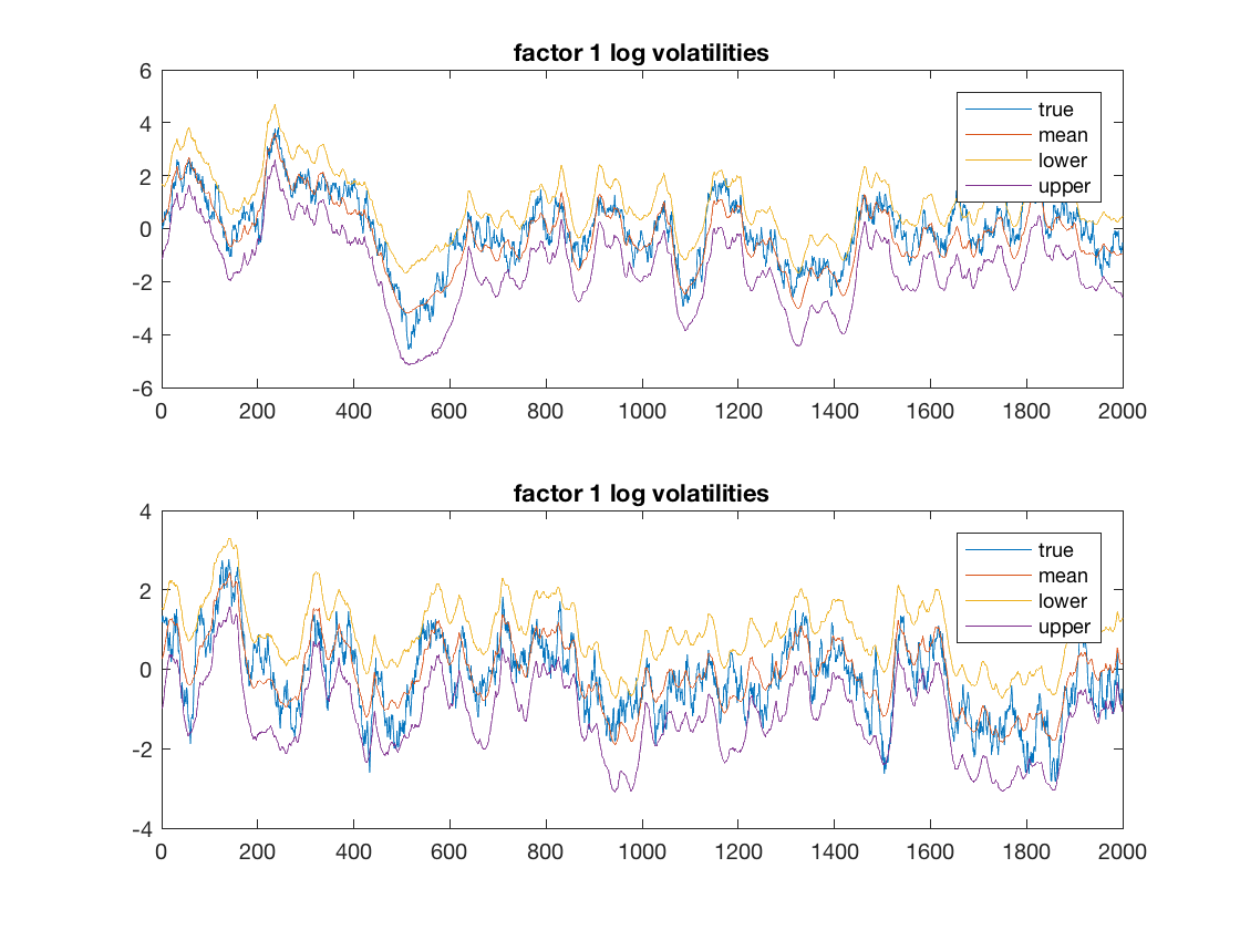
Tables 7, 8, and 9 in the Appendix show the inefficiency factors for all the parameters of factor MSV with leverage for the mixed, PG, and PGAS samplers, respectively. Table 1 summarises the simulation results and shows that the mixed sampler is more than 44 times more efficient than the PG sampler and more than 2 times more efficient than PGAS sampler. PGAS sampler is 2 times more efficient than PG sampler. Figures 1 and 2 show the estimated trajectory of idiosynchratic log-variances h1​s,th_{1s,t} for s=1,…,ps=1,...,p and factor log variances h2​j,th_{2j,t} for j=1,..,kj=1,..,k from mixed sampler. They estimate the true trajectory of idiosynchratic and factor log variances well.

Table 1: Comparison of Different Sampling Schemes. Time in seconds (N=500N=500) PG: Particle Gibbs, PGAS: Particle Gibbs with additional ancestor sampling step, Mix.: P​M​M​H​(τ112,…,τ1​p2,τ212,…,τ2​k2)+P​G​(μ1​s,ϕ1​s,ρ1​s,s=1,…,p,μ1​j,ϕ1​j,j=1,…,k,B,f)PMMH\left(\tau_{11}^{2},...,\tau_{1p}^{2},\tau_{21}^{2},...,\tau_{2k}^{2}\right)+PG\left(\mu_{1s},\phi_{1s},\rho_{1s},s=1,...,p;\mu_{1j},\phi_{1j},j=1,...,k;B,f\right).
PG PGAS Mix.
Time 1.07 1.18 1.75
I​A​C​TM​e​a​nIACT_{Mean} 70.45 31.05 10.42
TNV 75.38 36.64 18.23
Rel. TNV 4.13 2.01 1
Figure 1: Plots of estimated trajectories against the true trajectories of idiosynchratic log-variances h1​s,th_{1s,t} for s=1,…,10s=1,...,10
Refer to caption
Figure 2: Plot of estimated trajectories against the true trajectories of the factor log-variances h2​j,th_{2j,t} for j=1,…,2j=1,...,2
Refer to caption

5 Empirical Application to US stock returns

We applied the estimation described above to a sample of daily US stock returns. The data, provided by Kenneth French, consisted of the daily returns for 16 industry portfolios and it is given in Table 2. We used a sample running from 13rd August 1993 to 17th July 2001, a total of 2000 observations. We consider models with 1−41-4 factors. The total number of MCMC iterations is 1500015000, with the first 50005000 discarded as burn in replications. The number of particles is 10001000. Table 3 summarises the estimation results for 1−41-4 factors with standard normal prior N⁡(0,1)N\left(0,1\right) for each elements of factor loading matrix. It is clear that mixed sampler is always better than the PGAS sampler for all cases. Given the outcome of these comparisons, the remaining analysis are based on the results from the mixed sampler.

Table 2: List of Industry Portfolios
Industry Industry Industry Industry
1 Automobiles 5 Fabricated 9 Mining 13 Steel
2 Chemicals 6 Banks 10 Oil 14 Transportation
3 Textiles 7 Food 11 Other 15 Consumer Durables
4 Drugs, Soap, etc. 8 Machinery 12 Retail 16 Utilities
Table 3: Comparison of Different Sampling Schemes for Factor MSV with leverage. Time in seconds (N=1000N=1000)
1 Factor 2 Factor 3 factor 4 factor
PGAS Mixed PGAS Mixed PGAS Mixed PGAS Mixed
Time 2.63 4.35 2.65 4.40 2.70 4.45 2.75 4.50
I​A​C​TM​e​a​nIACT_{Mean} 132.04 15.96 122.04 16.69 111.42 29.76 146.11 26.01
TNV 347.27 69.43 323.41 73.44 300.83 132.43 401.80 117.05
Rel. TNV 5.00 1 4.40 1 2.27 1 3.43 1

In this paper, we select the number of factor using deviance information criterion (DIC). In the seminal paper, Spiegelhalter et al., (2002) proposed a concept of deviance information criterion (DIC) for model comparison. The model selection is based on the deviance, which is given by

D⁡(θ)=−2​log⁡p⁡(y|Θ)+2​log⁡h⁡(y),D\left(\theta\right)=-2\log p\left(y|\varTheta\right)+2\log h\left(y\right),

where p⁡(y|Θ)p\left(y|\varTheta\right) is the likelihood function of the parametric model and h⁡(y)h\left(y\right) is some fully specified standardising term that is only a function of the data. For model comparison purposes, we set h⁡(y)=1h\left(y\right)=1 for all models. The effective number of parameters pDp_{D} is defined as

pD=D⁡(θ)¯−D⁡(θ~),p_{D}=\overline{D\left(\theta\right)}-D\left(\tilde{\theta}\right),

where

D⁡(θ)¯=−2​Eθ​[log⁡p⁡(y|Θ)|y]+2​log⁡h⁡(y)\overline{D\left(\theta\right)}=-2E_{\theta}\left[\log p\left(y|\varTheta\right)|y\right]+2\log h\left(y\right)

is the posterior mean deviance and θ~\tilde{\theta} is an estimate of θ\theta, which is usually set to be posterior mode or mean. Thus, the deviance information criterion is defined as

D​I​C\displaystyle DIC =\displaystyle= D⁡(θ)¯+pD\displaystyle\overline{D\left(\theta\right)}+p_{D}
=\displaystyle= −4​Eθ​[log⁡p⁡(y|Θ)|y]+2​log⁡p⁡(y|θ~).\displaystyle-4E_{\theta}\left[\log p\left(y|\varTheta\right)|y\right]+2\log p\left(y|\tilde{\theta}\right).

Given a set of models for the given data, the preferred model is the one with the minimum DIC value. Celeux et al., (2006) pointed that there are a number of alternative definitions of the DIC in the latent variable models. In this paper, we follow the definitions of DIC that are based on conditional likelihood, which is given by:

D​I​C7=−4​Eθ,Z​[log⁡p⁡(y|Θ,Z)|y]+2​log⁡p⁡(y|Z^,θ^),DIC_{7}=-4E_{\theta,Z}\left[\log p\left(y|\varTheta,Z\right)|y\right]+2\log p\left(y|\widehat{Z},\widehat{\theta}\right),

where (Z^,θ^)\left(\widehat{Z},\widehat{\theta}\right) is the joint maximum a posterior (MAP) estimate, and ZZ consists of all the latent volatilities in the model. The first term on the right hand side can be estimated by averaging the log-conditional likelihoods log⁡p⁡(y|Θ,Z)\log p\left(y|\varTheta,Z\right) over the posterior draws of (Z,θ)\left(Z,\theta\right).

Table 4 shows the DIC values for 1-4 factors with different priors for elements of factor loading matrix. We compare standard normal prior N⁡(0,1)N\left(0,1\right), normal-gamma prior with as=1a_{s}=1 and as=0.5a_{s}=0.5 for all s=1,…,ps=1,...,p. We set the hyper-hyperparameters cs=ds=2c_{s}=d_{s}=2 for all s=1,…,ps=1,...,p. The best model is the four-factor model with normal-gamma prior (as=0.5)\left(a_{s}=0.5\right). We found no evidence for the leverage effects in the dataset, with posterior credible intervals of each ρs\rho_{s} including zero, except the mining industry. We begin by discussing the log-variances of the latent factors, visualised in Figure 3 and the corresponding posterior means of the factor loadings given in Table 6. The first factor can clearly be interpreted as the mining industry driven one. The automobiles, transportation and steel industries also load very highly on this factor. Factor 1’s log-variance appears quite volatile throughtout the sample period. Factor 2’s log variances appears slightly less volatile than the first factor, and generally very smooth and more persistent. It is also driven by mining industry. Retail and steel industries also loads very highly on this factor. The third factor volatility shows a similar overall pattern as the second. The fourth factor volatility shows a similar pattern as the first, but slightly more volatile. Figure 4 shows the marginal posterior means of univariate volatilities for all 1616 US stock returns from 13rd August 1993 to 17th July 2001. In general, the log-volatilities are generally smooth and less volatile, except, the fabricated, utilities, and bank industries.

Table 4: Selecting Number of Factors based on mixed sampler using DIC criterion
Number of Factors N⁡(0,1)N\left(0,1\right) prior N-G prior (as=1)\left(a_{s}=1\right) N-G prior (as=0.5)\left(a_{s}=0.5\right)
1 73893.3873893.38 73965.7273965.72 NA
2 72607.2572607.25 72466.7372466.73 NA
3 71594.4571594.45 71626.7871626.78 71490.1871490.18
4 71288.9571288.95 71334.7871334.78 71285.1771285.17
Table 5: The Inefficiency of factor loading matrix for different priors
Number of Factors N⁡(0,1)N\left(0,1\right) prior N-G prior (as=1)\left(a_{s}=1\right) N-G prior (as=0.5)\left(a_{s}=0.5\right)
3 18.6518.65 29.5629.56 22.4622.46
4 26.7726.77 27.0127.01 28.9528.95
Table 6: Posterior Means of factor loading matrix of four factor models with N-G prior (as=0.5)\left(a_{s}=0.5\right)
Automobiles 0.73 0 0 0
Chemicals 0.68 -0.59 0 0
Textiles 0.58 0.05 0.21 0
Drugs, Soap, etc. 0.58 0.48 -0.26 0.42
Fabricated 0.62 -0.01 0.21 0.03
Banks 0.56 -0.50 0.24 0.02
Food 0.71 0.21 0.17 0.19
Machinery 0.51 0.10 -0.32 0.38
Mining 0.83 0.71 1.61 0.11
Oil 0.39 -0.05 0.11 -0.11
Other 0.48 -0.59 -0.12 0.17
Retail 0.70 0.57 0.94 0.17
Steel 0.72 0.61 0.01 0.09
Transportation 0.72 -0.67 0.85 -0.10
Consumer Durables 0.70 -0.25 0.11 0.03
Utilities 0.33 -0.15 -0.16 0.21
Figure 3: Marginal Posteriors of the factor log-variances (m​e​a​n±2​s​d)(mean\pm 2sd), h2​j,th_{2j,t} for j=1,2,3,4j=1,2,3,4
Refer to caption
Figure 4: Posterior Volatilities of US Log returns (m​e​a​n±2​s​d)(mean\pm 2sd), h1​s,th_{1s,t} for s=1,…,16s=1,...,16
Refer to caption

6 Conclusions

Estimating time-varying covariance matrices of financial times series is an active area of research. In this paper, we employ factor multivariate stochastic volatility (factor MSV) models with leverage because they are able to model the volatility dynamics of a large system of financial or economic time series when the common features in these series can be captured by a small number of latent factors. To conduct efficient and reliable statistical inference, we propose a sampler based on recent developments in PMCMC methods. Our article demonstrates that a version of general PMCMC sampler of Mendes et al., (2016) provides a flexible and efficient framework to carry out inference on factor MSV models with leverage. The resulting parameter estimates mix well. The proposed method is illustrated using simulated and real datasets.

Appendix A Generic Sequential Monte Carlo (SMC) Algorithm

  1. 1.

    For t=1t=1

    1. (a)

      Sample h1ih_{1}^{i} from m1θ​(h)m_{1}^{\theta}\left(h\right), for i=1,…,Ni=1,...,N

    2. (b)

      Calculate the importance weights

      w1i=pθ​(y1|h1i)​pθ​(h1i)m1θ​(h1i),i=1,…,N.w_{1}^{i}=\frac{p_{\theta}\left(y_{1}|h_{1}^{i}\right)p_{\theta}\left(h_{1}^{i}\right)}{m_{1}^{\theta}\left(h_{1}^{i}\right)},i=1,...,N.

      and normalised them to obtain w¯11:N\overline{w}_{1}^{1:N}.

  2. 2.

    For t>1t>1

    1. (a)

      Sample the ancestral indices Ct−11:N∼M(a1:N|w¯t−11:N)C_{t-1}^{1:N}\sim M\left(a^{1:N}|\overline{w}_{t-1}^{1:N}\right).

    2. (b)

      Sample htih_{t}^{i} from mtθ​(ht|ht−1at−1i)m_{t}^{\theta}\left(h_{t}|h_{t-1}^{a_{t-1}^{i}}\right), i=1,…,Ni=1,...,N.

    3. (c)

      Set h1:t(i)=(h1:t−1(at−1i),ht(i))h_{1:t}^{\left(i\right)}=\left(h_{1:t-1}^{\left(a_{t-1}^{i}\right)},h_{t}^{\left(i\right)}\right).

    4. (d)

      Calculate the importance weights

      wti=pθ​(y1|hti)​pθ​(hti|ht−1at−1i)mtθ​(hti|ht−1at−1i),i=1,…,N.w_{t}^{i}=\frac{p_{\theta}\left(y_{1}|h_{t}^{i}\right)p_{\theta}\left(h_{t}^{i}|h_{t-1}^{a_{t-1}^{i}}\right)}{m_{t}^{\theta}\left(h_{t}^{i}|h_{t-1}^{a_{t-1}^{i}}\right)},i=1,...,N.

      and normalised them to obtain w¯t1:N\overline{w}_{t}^{1:N}.

Appendix B Conditional Sequential Monte Carlo

In the following, we describe the steps of conditional particle filter to draw (h1:T)\left(h_{1:T}\right) (Andrieu et al.,, 2010).

  1. 1.

    Fix h1:Tjh_{1:T}^{j} and C1:T−1jC_{1:T-1}^{j}.

  2. 2.

    For t=1t=1

    1. (a)

      Sample h1ih_{1}^{i} from m1θ​(h1)m_{1}^{\theta}\left(h_{1}\right), for i∈{1,…,N}∖{b1j}i\in\left\{1,...,N\right\}\setminus\left\{b_{1}^{j}\right\}.

    2. (b)

      Calculate the importance weights

      w1i=pθ​(y1|h1i)​pθ​(h1i)m1θ​(h1i),i=1,…,N.w_{1}^{i}=\frac{p_{\theta}\left(y_{1}|h_{1}^{i}\right)p_{\theta}\left(h_{1}^{i}\right)}{m_{1}^{\theta}\left(h_{1}^{i}\right)},i=1,...,N.

      and normalised them to obtain w¯11:N\overline{w}_{1}^{1:N}.

  3. 3.

    For t>1t>1

    1. (a)

      Sample the ancestral indices Ct−1−(btj)∼M(a(−btj)|w¯t−11:N)C_{t-1}^{-\left(b_{t}^{j}\right)}\sim M\left(a^{\left(-b_{t}^{j}\right)}|\overline{w}_{t-1}^{1:N}\right).

    2. (b)

      Sample htih_{t}^{i} from mtθ​(ht|ht−1at−1i)m_{t}^{\theta}\left(h_{t}|h_{t-1}^{a_{t-1}^{i}}\right), i=1,…,N∖{btj}i=1,...,N\setminus\left\{b_{t}^{j}\right\}.

    3. (c)

      Set h1:t(i)=(h1:t−1(at−1i),ht(i))h_{1:t}^{\left(i\right)}=\left(h_{1:t-1}^{\left(a_{t-1}^{i}\right)},h_{t}^{\left(i\right)}\right), i=1,…,Ni=1,...,N.

    4. (d)

      Calculate the importance weights

      wti=pθ​(y1|hti)​pθ​(hti|ht−1at−1i)mtθ​(hti|ht−1at−1i),i=1,…,N.w_{t}^{i}=\frac{p_{\theta}\left(y_{1}|h_{t}^{i}\right)p_{\theta}\left(h_{t}^{i}|h_{t-1}^{a_{t-1}^{i}}\right)}{m_{t}^{\theta}\left(h_{t}^{i}|h_{t-1}^{a_{t-1}^{i}}\right)},i=1,...,N.

      and normalised them to obtain w¯t1:N\overline{w}_{t}^{1:N}.

Appendix C Conditional Sequential Monte Carlo for Ancestral Sampling Algorithm

In the following, we describe the steps of conditional particle filter with ancestor sampling to draw (h1:T)\left(h_{1:T}\right) (Lindsten et al.,, 2014).

  1. 1.

    Fix h1:Tjh_{1:T}^{j} and C1:T−1jC_{1:T-1}^{j}.

  2. 2.

    For t=1t=1

    1. (a)

      Sample h1ih_{1}^{i} from m1θ​(h1)m_{1}^{\theta}\left(h_{1}\right), for i∈{,…,N}∖{b1j}i\in\left\{,...,N\right\}\setminus\left\{b_{1}^{j}\right\}.

    2. (b)

      Calculate the importance weights

      w1i=pθ​(y1|h1i)​pθ​(h1i)m1θ​(h1i),i=1,…,N.w_{1}^{i}=\frac{p_{\theta}\left(y_{1}|h_{1}^{i}\right)p_{\theta}\left(h_{1}^{i}\right)}{m_{1}^{\theta}\left(h_{1}^{i}\right)},i=1,...,N.

      and normalised them to obtain w¯11:N\overline{w}_{1}^{1:N}.

  3. 3.

    For t>1t>1

    1. (a)

      Sample the ancestral indices Ct−1−(btj)∼M(a(−btj)|w¯t−11:N)C_{t-1}^{-\left(b_{t}^{j}\right)}\sim M\left(a^{\left(-b_{t}^{j}\right)}|\overline{w}_{t-1}^{1:N}\right).

    2. (b)

      Draw bt−1(j)b_{t-1}^{\left(j\right)} from p⁡(bt−1(j)=k)∝wt−1(k)​pθ​(htbt(j)|ht−1(k))p\left(b_{t-1}^{\left(j\right)}=k\right)\propto w_{t-1}^{\left(k\right)}p_{\theta}\left(h_{t}^{b_{t}^{\left(j\right)}}|h_{t-1}^{\left(k\right)}\right).

    3. (c)

      Sample htih_{t}^{i} from mtθ​(ht|ht−1at−1i)m_{t}^{\theta}\left(h_{t}|h_{t-1}^{a_{t-1}^{i}}\right), i=1,…,N∖{btj}i=1,...,N\setminus\left\{b_{t}^{j}\right\}.

    4. (d)

      Calculate the importance weights

      wti=pθ​(y1|hti)​pθ​(hti|ht−1at−1i)mtθ​(hti|ht−1at−1i),i=1,…,N.w_{t}^{i}=\frac{p_{\theta}\left(y_{1}|h_{t}^{i}\right)p_{\theta}\left(h_{t}^{i}|h_{t-1}^{a_{t-1}^{i}}\right)}{m_{t}^{\theta}\left(h_{t}^{i}|h_{t-1}^{a_{t-1}^{i}}\right)},i=1,...,N.

      and normalised them to obtain w¯t1:N\overline{w}_{t}^{1:N}.

Appendix D Estimating Gradients of Log-Posterior using Particle Filter

This section presents the construction of the proposal density in Pseudo Marginal (PM) step that makes use of the derivatives of the log likelihood. Poyiadjis et al., (2011) were the first to show how the particle filter methods can be used to estimate the derivatives of the log likelihood for state space models. Their methods might suffer from a computational cost that is quadratic in the number of particles, Nemeth et al., (2016) proposed an alternative method whose computational cost is linear in the number of particles. They use a combination of kernel density estimation and Rao-Blackwellisation to reduce the Monte Carlo error of the estimates.

For non-linear and non-Gaussian state space models it is not possible to obtain the score and observed information matrix exactly. If it is possible to obtain a particle approximation of p(𝒉1:T|𝒚1:T,θ)p\left(\bm{h}_{1:T}|\bm{y}_{1:T},\theta\right), then this approximation can be used to estimate the score vector ∇logp(𝒚1:T|θ)\nabla\log p\left(\bm{y}_{1:T}|\theta\right) using Fisher’s identity (Cappe et al.,, 2005)

∇logp(𝒚1:T|θ)=∫∇logp(𝒉1:T,𝒚1:T|θ)p(𝒉1:T|𝒚1:T,θ)d𝒉1:T.\nabla\log p\left(\bm{y}_{1:T}|\theta\right)=\int\nabla\log p\left(\bm{h}_{1:T},\bm{y}_{1:T}|\theta\right)p\left(\bm{h}_{1:T}|\bm{y}_{1:T},\theta\right)d\bm{h}_{1:T}.

where

∇logp(𝒉1:T,𝒚1:T|θ)=∑t=1T{∇loggθ(𝒚t|𝒉t)+∇logpθ(𝒉t|𝒉t−1)}.\nabla\log p\left(\bm{h}_{1:T},\bm{y}_{1:T}|\theta\right)=\sum_{t=1}^{T}\left\{\nabla\log g_{\theta}\left(\bm{y}_{t}|\bm{h}_{t}\right)+\nabla\log p_{\theta}\left(\bm{h}_{t}|\bm{h}_{t-1}\right)\right\}.

The algorithm to estimate Gradient is given in (2).

Algorithm 2 Algorithm to estimate Gradient and Hessian Matrix Nemeth et al., (2016)
  • •

    Initialise: set m0(i)=0m_{0}^{\left(i\right)}=0 and n0(i)=0n_{0}^{\left(i\right)}=0 for i=1,…,Ni=1,...,N, where NN is the number of particles, and S0=0S_{0}=0 and B0=0B_{0}=0.

  • •

    At iteration t=1,…,Tt=1,...,T

    • –

      Run the Particle Filter to obtain {𝒉t(i)}i=1N\left\{\bm{h}_{t}^{\left(i\right)}\right\}_{i=1}^{N}, {ai}i=1N\left\{a_{i}\right\}_{i=1}^{N}, and {wt(i)}i=1N\left\{w_{t}^{\left(i\right)}\right\}_{i=1}^{N}, where wt(i)w_{t}^{\left(i\right)} is the weight of particle ii at time tt. aia_{i} is the ancestor index of particle ii at time t−1t-1.

    • –

      Normalised the weights Wt(i)=wt(i)∑wt(i)W_{t}^{\left(i\right)}=\frac{w_{t}^{\left(i\right)}}{\sum w_{t}^{\left(i\right)}}.

  • •

    Update the mt(i)m_{t}^{\left(i\right)} and nt(i)n_{t}^{\left(i\right)} as follows

    mt(i)=λ​mt−1(ki)+(1−λ)​St−1+∇log⁡gθ​(𝒚t|𝒉t(i))+∇log⁡pθ​(𝒉t(i)|𝒉t−1(ki))m_{t}^{\left(i\right)}=\lambda m_{t-1}^{\left(k_{i}\right)}+\left(1-\lambda\right)S_{t-1}+\nabla\log g_{\theta}\left(\bm{y}_{t}|\bm{h}_{t}^{\left(i\right)}\right)+\nabla\log p_{\theta}\left(\bm{h}_{t}^{\left(i\right)}|\bm{h}_{t-1}^{\left(k_{i}\right)}\right)
  • •

    Update the score vector

    St=∑i=1NWt(i)​mt(i)S_{t}=\sum_{i=1}^{N}W_{t}^{\left(i\right)}m_{t}^{\left(i\right)}

Setting λ=1\lambda=1 gives the Poyiadjis et al., (2011) algorithm. Nemeth et al., (2016) shows that bias and variance of both score estimate vary according to λ\lambda. Reducing the value of λ\lambda has the effect of increasing the bias, but it reduces the Monte Carlo variance of estimates. They also show that by setting λ≈0.95\lambda\approx 0.95 will produce an estimate for the score with linearly increasing variance and minimal bias. We use λ=0.95\lambda=0.95 in all our application.

Appendix E Sampling the scaling parameters in the deep interweaving representations

In the deep interweaving representation, we sample the scaling parameter Bj​jB_{jj} indirectly through μ2​j\mu_{2j}, j=1,…,kj=1,...,k. The implied prior p⁡(μ2​j)∝exp⁡(μ2​j/2−exp⁡(μ2​j)/2)p\left(\mu_{2j}\right)\propto\exp\left(\mu_{2j}/2-\exp\left(\mu_{2j}\right)/2\right) and the density p(B.,j∗|μ2​j)∼Nkj(0,exp(−μ2​j)Ikj)p\left(B_{.,j}^{*}|\mu_{2j}\right)\sim N_{k_{j}}\left(0,\exp\left(-\mu_{2j}\right)I_{k_{j}}\right) and the likelihood given by Equation (3) yields the posterior

p(μ2​j|B.,j∗,h2​j,.∗,ϕ2​j,τ2​j2)∝p(h2​j,.∗|μ2​j,ϕ2​j,τ2​j2)p(B.,j∗|μ2​j)p(μ2​j),p\left(\mu_{2j}|B_{.,j}^{*},h_{2j,.}^{*},\phi_{2j},\tau_{2j}^{2}\right)\propto p\left(h_{2j,.}^{*}|\mu_{2j},\phi_{2j},\tau_{2j}^{2}\right)p\left(B_{.,j}^{*}|\mu_{2j}\right)p\left(\mu_{2j}\right),

which is not in recognisable form. As in Kastner et al., (2017), we draw a proposal for μ2​jp​r​o​p\mu_{2j}^{prop} from N⁡(A,B)N\left(A,B\right) where

A=∑t=2T−1h2​j,t∗+(h2​j,T−ϕ2​j​h2​j,1)/(1−ϕ2​j)T+1/B0,B=τ2​j2/(1−ϕ2​j)2T+1/B0.A=\frac{\sum_{t=2}^{T-1}h_{2j,t}^{*}+\left(h_{2j,T}-\phi_{2j}h_{2j,1}\right)/\left(1-\phi_{2j}\right)}{T+1/B_{0}},B=\frac{\tau_{2j}^{2}/\left(1-\phi_{2j}\right)^{2}}{T+1/B_{0}}.

Denoting the current value μ2​j\mu_{2j} by μ2​jo​l​d\mu_{2j}^{old}, the new value μ2​jp​r​o​p\mu_{2j}^{prop} gets accepted with probability min⁡(1,R)\min\left(1,R\right), where

R=p(μ2​jp​r​o​p)p(h2​j,1∗|μ2​jp​r​o​p,ϕ2​j,τ2​j2)p(B.,j∗|μ2​jp​r​o​p)p(μ2​jo​l​d)(h2​j,1∗|μ2​jo​l​d,ϕ2​j,τ2​j2)p(B.,j∗|μ2​jo​l​d)×pa​u​x​(μ2​jo​l​d|ϕ2​j,τ2​j2)pa​u​x​(μ2​jp​r​o​p|ϕ2​j,τ2​j2),R=\frac{p\left(\mu_{2j}^{prop}\right)p\left(h_{2j,1}^{*}|\mu_{2j}^{prop},\phi_{2j},\tau_{2j}^{2}\right)p\left(B_{.,j}^{*}|\mu_{2j}^{prop}\right)}{p\left(\mu_{2j}^{old}\right)\left(h_{2j,1}^{*}|\mu_{2j}^{old},\phi_{2j},\tau_{2j}^{2}\right)p\left(B_{.,j}^{*}|\mu_{2j}^{old}\right)}\times\frac{p_{aux}\left(\mu_{2j}^{old}|\phi_{2j},\tau_{2j}^{2}\right)}{p_{aux}\left(\mu_{2j}^{prop}|\phi_{2j},\tau_{2j}^{2}\right)},

where

pa​u​x​(μ2​jo​l​d|ϕ2​j,τ2​j2)∼N⁡(0,B0​τ2​j2/(1−ϕ2​j)2).p_{aux}\left(\mu_{2j}^{old}|\phi_{2j},\tau_{2j}^{2}\right)\sim N\left(0,B_{0}\tau_{2j}^{2}/\left(1-\phi_{2j}\right)^{2}\right).

When normal-gamma prior is used, the density of B.,j∗|μ2​jB_{.,j}^{*}|\mu_{2j} is given by

p(B.,j∗|μ2​j)∼Nkj(0,Ψ.jexp(−μ2​j)),p\left(B_{.,j}^{*}|\mu_{2j}\right)\sim N_{k_{j}}\left(0,\Psi_{.j}\exp\left(-\mu_{2j}\right)\right),

where Ψ.j=diag(σ1​j2,…,σp​j2)\Psi_{.j}=diag\left(\sigma_{1j}^{2},...,\sigma_{pj}^{2}\right).

Appendix F Simulation Results

Table 7: Multivariate Factor SV model with leverage Simulation Results: Mixed Sampler with N=500N=500
IACT IACT IACT IACT IACT IACT
ϕ1\phi_{1} 12.16 τ12\tau_{1}^{2} 17.92 μ1\mu_{1} 1.89 ρ1\rho_{1} 12.31 β11\beta_{11} 6.33 β22\beta_{22} 5.86
ϕ2\phi_{2} 8.85 τ22\tau_{2}^{2} 16.43 μ2\mu_{2} 1.14 ρ2\rho_{2} 20.25 β21\beta_{21} 6.32 β23\beta_{23} 5.41
ϕ3\phi_{3} 11.51 τ32\tau_{3}^{2} 14.59 μ3\mu_{3} 1.36 ρ3\rho_{3} 23.23 β31\beta_{31} 6.46 β24\beta_{24} 6.24
ϕ4\phi_{4} 5.33 τ42\tau_{4}^{2} 15.88 μ4\mu_{4} 1.05 ρ4\rho_{4} 15.85 β41\beta_{41} 6.37 β25\beta_{25} 5.13
ϕ5\phi_{5} 4.70 τ52\tau_{5}^{2} 8.83 μ5\mu_{5} 1.02 ρ5\rho_{5} 30.09 β51\beta_{51} 6.44 β26\beta_{26} 5.12
ϕ6\phi_{6} 14.37 τ62\tau_{6}^{2} 19.56 μ6\mu_{6} 1.31 ρ6\rho_{6} 24.93 β61\beta_{61} 6.30 β27\beta_{27} 5.52
ϕ7\phi_{7} 6.78 τ72\tau_{7}^{2} 13.70 μ7\mu_{7} 1.10 ρ7\rho_{7} 37.98 β71\beta_{71} 6.32 β28\beta_{28} 5.84
ϕ8\phi_{8} 4.66 τ82\tau_{8}^{2} 9.25 μ8\mu_{8} 1.04 ρ8\rho_{8} 30.94 β81\beta_{81} 6.22 β29\beta_{29} 6.11
ϕ9\phi_{9} 6.17 τ92\tau_{9}^{2} 13.30 μ9\mu_{9} 1.04 ρ9\rho_{9} 30.43 β91\beta_{91} 5.72 β2,10\beta_{2,10} 6.27
ϕ10\phi_{10} 8.12 τ102\tau_{10}^{2} 16.65 μ10\mu_{10} 1.45 ρ10\rho_{10} 19.90 β10,1\beta_{10,1} 6.26
ϕf​1\phi_{f1} 10.36 τf​12\tau_{f1}^{2} 12.64
ϕf​2\phi_{f2} 13.96 τf​22\tau_{f2}^{2} 18.24
Table 8: Multivariate Factor SV model with leverage Simulation Results: PG Sampler with N=500N=500
IACT IACT IACT IACT IACT IACT
ϕ1\phi_{1} 87.72 τ12\tau_{1}^{2} 229.96 μ1\mu_{1} 3.07 ρ1\rho_{1} 17.16 β11\beta_{11} 5.31 β22\beta_{22} 7.17
ϕ2\phi_{2} 128.27 τ22\tau_{2}^{2} 273.72 μ2\mu_{2} 1.04 ρ2\rho_{2} 23.46 β21\beta_{21} 5.47 β23\beta_{23} 6.71
ϕ3\phi_{3} 96.86 τ32\tau_{3}^{2} 188.35 μ3\mu_{3} 1.64 ρ3\rho_{3} 32.85 β31\beta_{31} 5.43 β24\beta_{24} 6.05
ϕ4\phi_{4} 83.42 τ42\tau_{4}^{2} 336.61 μ4\mu_{4} 1.02 ρ4\rho_{4} 24.44 β41\beta_{41} 5.39 β25\beta_{25} 4.94
ϕ5\phi_{5} 30.09 τ52\tau_{5}^{2} 214.09 μ5\mu_{5} 1.08 ρ5\rho_{5} 40.87 β51\beta_{51} 5.39 β26\beta_{26} 6.26
ϕ6\phi_{6} 271.72 τ62\tau_{6}^{2} 510.85 μ6\mu_{6} 1.23 ρ6\rho_{6} 32.51 β61\beta_{61} 5.44 β27\beta_{27} 7.24
ϕ7\phi_{7} 53.51 τ72\tau_{7}^{2} 234.28 μ7\mu_{7} 1.12 ρ7\rho_{7} 45.32 β71\beta_{71} 5.45 β28\beta_{28} 7.64
ϕ8\phi_{8} 27.35 τ82\tau_{8}^{2} 174.22 μ8\mu_{8} 1.02 ρ8\rho_{8} 30.07 β81\beta_{81} 5.48 β29\beta_{29} 7.52
ϕ9\phi_{9} 49.86 τ92\tau_{9}^{2} 188.67 μ9\mu_{9} 1.02 ρ9\rho_{9} 42.76 β91\beta_{91} 5.28 β2,10\beta_{2,10} 7.92
ϕ10\phi_{10} 95.05 τ102\tau_{10}^{2} 259.60 μ10\mu_{10} 1.17 ρ10\rho_{10} 19.33 β10,1\beta_{10,1} 6.34
ϕf​1\phi_{f1} 42.32 τf​12\tau_{f1}^{2} 121.84
ϕf​2\phi_{f2} 99.06 τf​22\tau_{f2}^{2} 202.43
Table 9: Multivariate Factor SV model with leverage Simulation Results: PGAS Sampler with N=500N=500
IACT IACT IACT IACT IACT IACT
ϕ1\phi_{1} 44.55 τ12\tau_{1}^{2} 100.13 μ1\mu_{1} 1.26 ρ1\rho_{1} 9.56 β11\beta_{11} 5.53 β22\beta_{22} 7.20
ϕ2\phi_{2} 22.34 τ22\tau_{2}^{2} 81.51 μ2\mu_{2} 1.18 ρ2\rho_{2} 14.33 β21\beta_{21} 5.54 β23\beta_{23} 4.81
ϕ3\phi_{3} 57.44 τ32\tau_{3}^{2} 100.61 μ3\mu_{3} 1.36 ρ3\rho_{3} 18.13 β31\beta_{31} 5.67 β24\beta_{24} 5.79
ϕ4\phi_{4} 34.07 τ42\tau_{4}^{2} 126.11 μ4\mu_{4} 1.02 ρ4\rho_{4} 11.96 β41\beta_{41} 5.56 β25\beta_{25} 5.30
ϕ5\phi_{5} 24.27 τ52\tau_{5}^{2} 72.48 μ5\mu_{5} 1.11 ρ5\rho_{5} 24.22 β51\beta_{51} 5.61 β26\beta_{26} 6.92
ϕ6\phi_{6} 49.25 τ62\tau_{6}^{2} 103.15 μ6\mu_{6} 1.22 ρ6\rho_{6} 21.72 β61\beta_{61} 5.50 β27\beta_{27} 7.49
ϕ7\phi_{7} 20.92 τ72\tau_{7}^{2} 61.51 μ7\mu_{7} 1.04 ρ7\rho_{7} 20.34 β71\beta_{71} 5.53 β28\beta_{28} 7.94
ϕ8\phi_{8} 17.76 τ82\tau_{8}^{2} 83.77 μ8\mu_{8} 1.04 ρ8\rho_{8} 22.47 β81\beta_{81} 5.46 β29\beta_{29} 8.58
ϕ9\phi_{9} 24.50 τ92\tau_{9}^{2} 72.55 μ9\mu_{9} 1.04 ρ9\rho_{9} 17.18 β91\beta_{91} 5.02 β2,10\beta_{2,10} 10.17
ϕ10\phi_{10} 69.57 τ102\tau_{10}^{2} 184.45 μ10\mu_{10} 1.19 ρ10\rho_{10} 12.84 β10,1\beta_{10,1} 5.74
ϕf​1\phi_{f1} 21.62 τf​12\tau_{f1}^{2} 68.15
ϕf​2\phi_{f2} 65.94 τf​22\tau_{f2}^{2} 146.21

References

  • Aguilar and West, (2000) Aguilar, O. and West, M. (2000). Bayesian dynamic factor models and portfolio allocation. Journal of Business and Economics Statistics, 18(3):338–357.
  • Andrieu et al., (2010) Andrieu, C., Doucet, A., and Holenstein, R. (2010). Particle Markov chain Monte Carlo methods. Journal of the Royal Statistical Society, Series B, 72:1–33.
  • Bollerslev et al., (1994) Bollerslev, T., Engle, R. F., and Nelson, D. B. (1994). ARCH Models, volume 4, 2959-3038. The Handbook of econometrics, North Holland, Amsterdam.
  • Cappe et al., (2005) Cappe, O., Moulines, E., and Ryden, T. (2005). Inference in Hidden Markov Models. Springer Series in Statistics.
  • Celeux et al., (2006) Celeux, G., Forbes, F., Robert, C. P., and Titterington, D. M. (2006). Deviance information criteria for missing data models. Bayesian Analysis, 1(4):651–674.
  • Chib et al., (2006) Chib, S., Nardari, F., and Shephard, N. (2006). Analysis of high dimensional multivariate stochastic volatility models. Journal of Econometrics, 134:341–371.
  • Chopin and Singh, (2013) Chopin, N. and Singh, S. S. (2013). On the particle Gibbs sampler. Working paper, eprint arXiv:1304.1887.
  • Geweke and Zhou, (1996) Geweke, J. F. and Zhou, G. (1996). Measuring the pricing error of the arbitrage pricing theory. Review of Financial Studies, 9:557–587.
  • Ghysels et al., (1996) Ghysels, E., Harvey, A. C., and Renault, E. (1996). Stochastic volatility. Statistical Methods in Finance, North Holland, Amsterdam, pages 119–191.
  • Gordon et al., (1993) Gordon, N., Salmond, D., and Smith, A. (1993). A novel approach to nonlinear and non-Gaussian Bayesian state estimation. IEE-Proceedings F, 140:107–113.
  • Griffin and Brown, (2010) Griffin, J. E. and Brown, P. J. (2010). Inference with normal-gamma prior distribution in regression problems. Bayesian Analysis, 5(1):171–188.
  • Han, (2006) Han, Y. (2006). Asset allocation with a high dimensional latent factor stochastic volatility model. Review of Financial Studies, 19(1):237–271.
  • Harvey and Shephard, (1996) Harvey, A. C. and Shephard, N. (1996). The estimation of an asymmetric stochastic volatility model for an asset returns. Journal of Business and Economics Statistics, 14:429–434.
  • Hoffman and Gelman, (2014) Hoffman, M. D. and Gelman, A. (2014). The No-U-Turn sampler: adaptively setting path length in Hamiltonian Monte Carlo. Journal of Machine Learning Research, 15:1593–1623.
  • Kastner et al., (2017) Kastner, G., Schnatter, S. F., and Lopes, H. F. (2017). Efficient bayesian inference for multivariate factor stochastic volatility models. Journal of Computational and Graphical Statistics.
  • Kim et al., (1998) Kim, S., Shephard, N., and Chib, S. (1998). Stochastic volatility: Likelihood inference and comparison with arch models. The Review of Economic Studies, 65(3):361–393.
  • Kitagawa, (1996) Kitagawa, G. (1996). Monte Carlo filter and smsmooth for non-Gaussian nonlinear state space models. Journal of Computational and Graphical Statistics, 5(1):1–25.
  • Lindsten et al., (2014) Lindsten, F., Jordan, M. I., and Schon, T. B. (2014). Particle Gibbs with ancestor sampling. Journal of Machine Learning Research, 15:2145–2184.
  • Liu, (2001) Liu, J. S. (2001). Monte Carlo strategies in scientific computing. New York: Springer.
  • Lopes and West, (2004) Lopes, H. F. and West, M. (2004). Bayesian model assessment in factor analysis. Statistica Sinica, pages 41–67.
  • Mendes et al., (2016) Mendes, E. F., Carter, C. K., and Kohn, R. (2016). On general sampling schemes for Particle Markov chain Monte Carlo. arXiv preprint arXiv:1401.1667v3.
  • Neal, (1996) Neal, R. M. (1996). Bayesian Learning for Neural Networks. Springer, Lecture Notes in Statistics, New York.
  • Neal, (2011) Neal, R. M. (2011). MCMC using Hamiltonian dynamics. Handbook of Markov chain Monte Carlo.
  • Nemeth et al., (2016) Nemeth, C., Fearnhead, P., and Mihaylova, L. S. (2016). Particle approximations of the score and observed information matrix for parameter estimation in state space models with linear computational cost. Journal of Computational and Graphical Statistics, 25(4):1138–1157.
  • Nesterov, (2009) Nesterov, Y. (2009). Primal-dual subgradient methods for convex problems. Mathematical programming, 120(1):221–259.
  • Omori et al., (2007) Omori, Y., Chib, S., Shephard, N., and Nakajima, J. (2007). Stochastic volatility with leverage: Fast and efficient likelihood inference. Journal of Econometrics, 140:425–449.
  • Park and Casella, (2008) Park, T. and Casella, G. (2008). The bayesian lasso. Journal of the American Statistical Association, 103:681–686.
  • Pitt and Shephard, (1999) Pitt, M. and Shephard, N. (1999). Filtering via simulation:auxiliary particle filter. Journal of American Statistical Association, 94:590–599.
  • Poyiadjis et al., (2011) Poyiadjis, G., Doucet, A., and Singh, S. S. (2011). Particle aapproximation of the score and observed information matrix in state space models with application to parameter estimation. Biometrika, 98(1):65–80.
  • Roberts and Stramer, (2003) Roberts, G. and Stramer, O. (2003). Langevin diffusions and Metropolis-Hastings algorithm. Methodology and Computing in Applied Probability, 4:337–358.
  • Scharth and Kohn, (2016) Scharth, M. and Kohn, R. (2016). Particle efficient importance sampling. Journal of Econometrics, 190(1):133–147.
  • Spiegelhalter et al., (2002) Spiegelhalter, D. J., Best, N. G., Carlin, B. P., and van der Linde, A. (2002). Bayesian measures of model complexity and fit. Journal of Royal Statistician Society Series B, 64(4):583–639.